Grace O. Akinlabi*![]() | Henry E. Egbogho
| Henry E. Egbogho![]()
© 2024 The authors. This article is published by IIETA and is licensed under the CC BY 4.0 license (http://creativecommons.org/licenses/by/4.0/).
OPEN ACCESS
Vibration is a mechanical phenomenon that causes oscillations around an equilibrium point. Vibration is undesired in many areas, particularly engineered systems and inhabited spaces, and strategies to avoid vibration transfer to such systems have been proposed. Mechanical waves carry vibrations, and certain mechanical couplings transport vibrations more efficiently than others. By detecting equipment defects, vibration analysis (VA) in an industrial or maintenance setting seeks to save maintenance costs and downtime. Associated models from vibration settings can either be linear or nonlinear based on the modeling situation. This paper considers the Zhou Transform Method (ZTM) as a semi-analytical approach for obtaining the solutions of linear vibration mechanical models. Two illustrative examples are considered. The results obtained from the ZTM are compared with their exact forms for applicable case(s). The results show that the proposed method is very effective and reliable in obtaining approximate solutions based on the comparison.
vibration model, differential equation, approximate-analytical solutions
Vibrations in dynamic mechanical systems are oscillations [1]. While when compelled to do so externally, every device can oscillate. The word 'vibration' is always reserved in mechanical engineering for devices (machines, tools, or systems) that can oscillate freely without applied forces. Often in designed structures, these movements trigger mild to significant output or protection concerns. The mechanical vibration analysis task should be to use mathematical methods that are typically not apparent in preliminary engineering designs for modeling and predicting possible vibration problems and solutions. If problems can be expected, so prototypes can be changed before such devices are produced to minimize vibration problems. Vibrations may even be purposely incorporated into designs and systems in order to take advantage of relative mechanical motion and rebound structures. Unfortunately, knowledge of vibrations is seldom considered necessary in preliminary mechanical projects, so often, vibration experiments are conducted only after devices are produced. Vibration issues must be solved in both situations using passive or active interface changes. In nearly all branches of engineering, vibrations can arise, and the methods here can be readily generalized to other circumstances, typically with only a shift of notation [2, 3]. Vibration or dynamic mechanical systems are mainly differential equations whose solutions need to be interpreted meaningfully, only if they can be obtained.
Structural engineers strive to be very interested in the dynamic characteristics of bridges that are subjected to the passage of moving vehicles. The nonlinear strain models, in which the axial strains and transverse displacements are coupled, cause nonlinearity in beams and plates. Meanwhile, in a dynamical analysis of vibration models, it was noted that optimum linear and cubic nonlinear vibration absorbers are the results of an effective application of a linear beam structure [4]. Hence, proper knowledge of the linear version of the vibration model is vital. On the method of solution, an effective technique that could handle both linear and nonlinear systems with ease is required for adoption, as proposed in this study.
Should the solution exist, it is necessary to use dependable solution algorithms in order to acquire approximate or theoretical solutions to different types of differential equations or systems [5-10]. For effectiveness and dependability, some researchers have created iterative methods or improved upon already-existing ones. Examples include the Homotopy Perturbation Method, the New Iterative Method (NIM), the Picard Iterative Method (PIM), the Adomian Decomposition Method (ADM), the Variational Iterative Method (VIM), the Boundary Value Techniques, and others [11-26]. The Zhou Transformation Method (ZTM), most often referred to as the differential transformation method, is introduced in this study as a semi-analytical technique for linear vibration mechanical models' solutions.
As regards the findings in this study, is clear that the proposed method is very viable as the approximate results coincide with their exact forms when compared and demonstrated graphically. Since the method ensures dependability and efficiency, it is noted that the solutions can reasonably be approximated without complexity.
The paper structure is as follows: In Section 1, the basic introduction is presented; Section 2 handles the concerned vibration model; Section 3 deals with the method of solution and its properties; Section 4 presents illustrative examples; and in Section 5, a remark on the discussion and conclusion of the results is presented.
The governing vibration model is discussed using the following Figure 1 according to the study [2].
Figure 1. Mechanical vibration chart (Zachary [2])
Suppose we denote displacement by u(t)=w(t) as a function of time, with a mass relative to the corresponding equilibrium position, which implies that w=w(t)>0 entails that the spring is stretched outside (beyond) the required equilibrium. As such, w<0 implies a compressed spring.
We make reference to related works as depicted in references [4, 27-29]. By assumption, the mass is set in motion. Thus, at equilibrium (by Hooke's law) and in motion, we have the following respectively [2]:
$\left. \begin{align} & mg=kL \\ & m{w}''\left( t \right)+\xi {w}'\left( t \right)+kw\left( t \right)=H\left( t \right) \\\end{align} \right\}$ (1)
where, m>0 is mass, ξ≥0 is the damping constant, k>0 is the spring, L is the spring elongation engendered by the weight, g is the gravitational constant, H(t) implies an externally applied function, while w(t0), and w'(t0) are initial displacement and initial velocity of the mass, respectively.
A case of undamped free vibration is encountered when ξ=0 & H(t)=0 which gives the simplest mechanical vibration of the form [2]:
$m{w}''\left( t \right)+kw\left( t \right)=0$ (2)
In this study, cases of damped free vibration (that is when ξ>0 & H(t)=0) are considered. This yields the motion equation of an unforced mass-spring model.
Remark:
(i) An item (object) that is falling freely is one that is just being affected by gravity. This means that any moving object that is simply being affected by gravity is said to be "in a state of free fall." An item of this kind will accelerate downward at a rate of 9.8 m/s/s. If the item is just subject to the effects of gravity, whether it is scaling upward or falling toward its peak, its acceleration value is 9.8 m/s/s.
(ii) When the mass is pulled downward, it entails the initial condition (position), w(0)>0. Meanwhile, when the mass is released from rest, it implies that the initial velocity w'(0)=0. In addition, when the mass is pushed (released) downward, it implies the initial velocity, w'(0)>0.
This section presents the idea of the Zhou Method as applied to some classes of the unforced mass-spring vibration model.
3.1 Analysis of the ZTM
The method (ZTM), as found out by several scholars, has been shown to allow applications for dynamical models (linear or nonlinear), provided that the DTM translates the problems involved into their counterparts in recursive algebraic forms. However, this is not so where other semi-analytical methods, such as ADM, PIM, HAM, VIM and so on, are used. The Zhou method has been modified to handle higher-order nonlinear models and their related likes [30-32].
3.2 The overview of the DTM
Let p(t) be a differentiable and continuous function with transformed form given as p(k). Hence, the k-th derivative of p(t) is denoted as:
$P\left( k \right)=\frac{1}{k!}{{\left( \frac{{{d}^{k}}p\left( t \right)}{d{{t}^{k}}} \right)}_{t={{t}_{0}}}}$ (3)
So, the inverse form of P(k) is:
$p\left( t \right)=\sum\limits_{k=0}^{\infty }{P\left( k \right){{\left( t-{{t}_{0}} \right)}^{k}}}$ (4)
Using Eq. (3) in Eq. (4) therefore gives:
$p\left( t \right)=\left\{ \begin{align} & \sum\limits_{j=0}^{\infty }{\frac{{{\left( t-{{t}_{0}} \right)}^{j}}}{j!}{{\left( \frac{{{d}^{j}}p\left( t \right)}{d{{t}^{j}}} \right)}_{t={{t}_{0}}}},\text{ }{{t}_{0}}\ne 0} \\ & \sum\limits_{j=0}^{\infty }{\frac{{{t}^{j}}}{j!}{{\left( \frac{{{d}^{j}}p\left( t \right)}{d{{t}^{j}}} \right)}_{t=0}}},\text{ }{{t}_{0}}=0 \\\end{align} \right.$ (5)
Table 1. Some main features of the Zhou method
|
Property |
Original Function Form |
Transformed Function (Zhou) |
|
P1 |
$m(t)=\alpha m_a(t) \pm \beta m_b(t)$ |
$M(k)=\alpha M_a(k) \pm \beta M_b(k)$ |
|
P2 |
$m(t)=\frac{\alpha d^\eta m_{+}(t)}{d t^\eta}, \eta \in \mathbb{N}$ |
$M(k)=\frac{\alpha(k+\eta)!}{k!} M_{+}(k+\eta)$ |
|
P3 |
$m(t)=e^{\lambda t}$ |
$M(k)=\frac{\lambda^k}{k!}$ |
|
P4 |
$m(t)=m_{+}^2(t)$ |
$M(k)=\sum_{\eta=0}^k M_{+}(\eta) M_{+}(k-\eta)$ |
3.3 The fundamentals of ZTM: Theorems and properties
In Table 1, the properties and theorems linked with the method are presented (P1-P4).
The readers are to see references [28-30] for more details of the proposed method, even for non-integer calculus.
Eq. (5) implies that the transformation method was obtained from the expansion of the Taylor series.
Example 4(a)
Suppose a spring of 0.1m is stressed by a mass of 1kg, while the system possesses a damping constant of ξ=14, such that at time, t=0, the concerned mass is pulled down (1m), and released with a downward velocity of -4.5m/s. Thus, the following are induced:
$\left\{\begin{array}{l}m=1, \xi=14, L=0.1 \\ m g=9.8 \Rightarrow k=98\end{array}\right.$ (6)
In this case, the damped free vibration (motion) equation is given as:
$\left\{ \begin{align} & {w}''\left( t \right)+14{w}'\left( t \right)+98w\left( t \right)=0, \\ & w(0)=1,\text{ }{w}'\left( 0 \right)=4.5 \\\end{align} \right.$ (7)
Applying the proposed method transforms (7) to:
$\left. \begin{align} & ~W\left( j+2 \right)=-\frac{\left\{ 14\left( j+1 \right)W\left( j+1 \right)+98W\left( j \right) \right\}}{\left( j+1 \right)\left( j+2 \right)},\text{ } \\ & j=0,1,2,\cdots W(0)=1,\text{ }W\left( 1 \right)=4.5 \\\end{align} \right\}$ (8)
Thus, the following are obtained:
$\left\{ \begin{align} & W(0)=1,\text{ }W(1)=4.5,\text{ } \\ & W\left( 2 \right)=-80.50000000, \\ & W\left( 3 \right)=302.1666667,\text{ } \\ & W\left( 4 \right)=-400.1666667, \\ & W\left( 5 \right)=-360.1500000,\text{ } \\ & W\left( 6 \right)=2147.561111, \\ & W\left( 7 \right)=-3454.772221,\text{ } \\ & W\left( 8 \right)=2287.619443 \\\end{align} \right.$ (9)
The solution of (6) is therefore given as:
$\begin{align} & w\left( t \right)=\underset{N\to \infty }{\mathop{\lim }}\,\left( \sum\limits_{j=0}^{N}{W\left( j \right){{t}^{j}}} \right)=1+4.5t+406.6202583{{t}^{16}} \\ & +107.6347740{{t}^{17}}-213.9407239{{t}^{18}}+126.7978204{{t}^{19}} \\ & -33.58428761{{t}^{20}}-7.196633022{{t}^{21}}+11.70361535{{t}^{22}} \\ & -5.730125478{{t}^{23}}+1.264757428{{t}^{24}}+0.2276563350{{t}^{25}} \\ & -0.3132706849{{t}^{26}}+0.1306555676{{t}^{27}} \\ & -0.02471862094{{t}^{28}}-0.003835648044{{t}^{29}} \\ & +0.004574365469{{t}^{30}}+4189.347527{{t}^{11}} \\ & -1849.351610{{t}^{12}}-640.1601737{{t}^{13}}+1635.964887{{t}^{14}} \\ & -1228.159147{{t}^{15}}+1143.809724{{t}^{9}}-4092.297007{{t}^{10}} \\ & -80.50000000{{t}^{2}}+302.1666667{{t}^{3}}-400.1666667{{t}^{4}} \\ & -360.1500000{{t}^{5}}+2147.561111{{t}^{6}}-3454.772221{{t}^{7}} \\ & +2287.619443{{t}^{8}} \\\end{align}$ (10)
Figure 2. Graphic solution for Example 4(a)
Example 4(b)
Consider a critically damped Initial Value Problem (IVP) of the form:
$\left\{ \begin{align} & {w}''\left( t \right)+6{w}'\left( t \right)+9w\left( t \right)=0, \\ & w(0)={w}'\left( 0 \right)=1, \\ & w(t)=\left( 1+4t \right)\exp \left( -3t \right)\text{, (exact root)}\text{.} \\\end{align} \right.$ (11)
Applying the proposed method transforms (11) to:
$\left. \begin{align} & ~W\left( j+2 \right)=-\frac{\left\{ 6\left( j+1 \right)W\left( j+1 \right)+9W\left( j \right) \right\}}{\left( j+1 \right)\left( j+2 \right)}, \\ & \text{ }j=0,1,2,\cdots ,\text{ }W(0)=1,\text{ }W\left( 1 \right)=1. \\\end{align} \right\}$ (12)
Thus, the following are obtained:
$\left\{ \begin{align} & W(0)=1,\text{ }W(1)=1,\text{ }W(2)=\frac{-15}{2},\text{ }W(3)=\frac{27}{2}, \\ & W(4)=\frac{-117}{8},\text{ }W(5)=\frac{459}{40},\text{ }W(6)=\frac{-567}{80}, \\ & W(7)=\frac{450}{112},\text{ }W(8)=\frac{-7047}{4480},\text{ }W(9)=\frac{2673}{4480}\text{,} \\ & W(10)=\frac{-8991}{44800},\text{ }W(11)=\frac{29889}{492800},\text{ }\cdots \\\end{align} \right.$ (13)
The solution of (11) is therefore given as:
$\begin{align} & w\left( t \right)=\underset{N\to \infty }{\mathop{\lim }}\,\left( \sum\limits_{j=0}^{N}{W\left( j \right){{t}^{j}}} \right)\text{ }=1+t-\frac{15}{2}{{t}^{2}}+\frac{27}{2}{{t}^{3}}-\frac{117}{8}{{t}^{4}} \\ & +\frac{459}{40}{{t}^{5}}-\frac{567}{80}{{t}^{6}}+\frac{405}{112}{{t}^{7}}-\frac{7047}{4480}{{t}^{8}}+\frac{2673}{4480}{{t}^{9}}-\frac{8991}{44800}{{t}^{10}} \\ & +\frac{29889}{492800}{{t}^{11}}-\frac{6561}{394240}{{t}^{12}}+\frac{15309}{3660800}{{t}^{13}}-\frac{347733}{358758400}{{t}^{14}} \\ & +\frac{373977}{1793792000}{{t}^{15}}-\frac{1200663}{28700672000}{{t}^{16}}+\frac{59049}{7506329600}{{t}^{17}} \\ & -\frac{1358127}{975822848000}{{t}^{18}}+\frac{4310577}{18540634112000}{{t}^{19}}-\frac{177147}{4815749120000}{{t}^{20}} \\ & +\frac{14348907}{2595688775680000}{{t}^{21}}-\frac{531441}{671825330176000}{{t}^{22}} \\ & +\frac{141894747}{1313418520494080000}{{t}^{23}}-\frac{148272039}{10507348163952640000}{{t}^{24}}+\cdots . \\\end{align}$ (14)
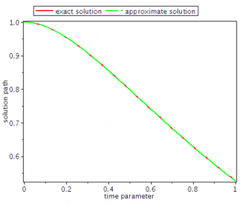
Figure 3. Graphic solution for Example 4(b)
In Figure 2 and Figure 3, the graphical solutions are presented with respect to the obtained and the exact solutions. These aid in the comparison of the solutions.
Example 4(c)
Consider an overdamped Initial Value Problem (IVP) of the form:
$\left\{ \begin{align} & {w}''\left( t \right)+4{w}'\left( t \right)+3w\left( t \right)=0,\text{ }w(0)=1,\text{ }{w}'\left( 0 \right)=0, \\ & w(t)=\frac{1}{2}\left( 3\exp \left( -t \right)-\exp \left( -3t \right) \right)\text{, (exact root)}\text{.} \\\end{align} \right.$ (15)
Applying the proposed method transforms (15) to:
$\left. \begin{align} & ~W\left( j+2 \right)=-\frac{\left\{ 4\left( j+1 \right)W\left( j+1 \right)+3W\left( j \right) \right\}}{\left( j+1 \right)\left( j+2 \right)}, \\ & j=0,1,2,\cdots ,\text{ }W(0)=1,\text{ }W\left( 1 \right)=0. \\\end{align} \right\}$ (16)
Thus, the following are obtained:
$\left\{ \begin{align} & W(0)=1,\text{ }W(1)=0,\text{ }W(2)=-\frac{3}{2},\text{ } \\ & W(3)=2,\text{ }W(4)=-\frac{13}{8},\text{ }W(5)=-\frac{121}{240},\text{ } \\ & W(6)=-\frac{121}{240},\text{ }W(7)=\frac{13}{60},\text{ }W(8)=-\frac{1093}{13440}, \\ & W(9)=\frac{41}{1512}\text{, }W(10)=-\frac{9841}{1209600}, \\ & W(11)=\frac{671}{302400},\text{ }\cdots \\\end{align} \right.$ (17)
The solution of (15) is therefore given as:
$\left. \begin{align} & w\left( t \right)=\underset{N\to \infty }{\mathop{\lim }}\,\left( \sum\limits_{j=0}^{N}{W\left( j \right){{t}^{j}}} \right)\text{ } \\ & =1-\frac{3}{2}{{t}^{2}}+2{{t}^{3}}-\frac{13}{8}{{t}^{4}}+{{t}^{5}}-\frac{121}{240}{{t}^{6}} \\ & +\frac{13}{60}{{t}^{7}}-\frac{1093}{13440}{{t}^{8}}+\frac{41}{1512}{{t}^{9}}-\frac{9841}{1209600}{{t}^{10}} \\ & +\frac{671}{302400}{{t}^{11}}-\frac{88573}{159667200}{{t}^{12}}+\cdots . \\\end{align} \right\}$ (18)
Figure 4. Graphic solution for Example 4(c)
In Figure 4, the graphical representation of the problem (Example 4(c)) in terms of solutions in is presented. The convergence of the solutions can easily be observed.
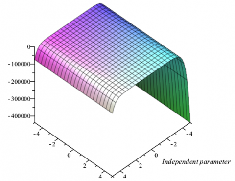
We wish to state here that the convergence of the approximate solutions to the exact solutions when the proposed method is applied strongly depends on the level and number of iterations involved. This can be seen clearly from Figures 5 and 6 for the exact and approximate solutions, respectively, regarding Example 4(c). Figure 6 is a 12-term approximate solution to the problem.
Figure 5. Path-view of the exact solution of Example 4(c)
Figure 6. Path-view of the approx. solution of Example 4(c)
In this work, we have successfully used the Zhou method to obtain the solution of linear vibration mechanical models. The results obtained from the proposed method are compared with their exact forms. It is remarked that the results or solutions can reasonably be approximated with less effect since the method ensures reliability and efficiency; these are obvious from the graphical solutions shown in the figures. Some of the primary advantages of the Zhou method include its ease of application and reduction of computational work. This model can be extended to non-integer variants either in time, space, of time-space fractional while the method is employed for the prediction of the associated or resulting vibration engendered by the fractional model.
The authors sincerely appreciate Covenant University for the provision of a conducive working environment.
|
W |
displacement |
|
M |
mass, kg |
|
g |
gravitational constant |
|
k |
spring |
|
L |
spring elongation |
|
H |
externally applied function |
|
t |
time |
|
p(t) |
continuous and differentiable function |
|
P(K) |
transformed form of p(t) |
|
w(t0) |
initial displacement of the mass |
|
W'(t0) |
initial velocity of the mass |
|
Greek symbols |
|
|
$\alpha$ |
arbitrary constant |
|
$\beta$ |
arbitrary constant |
|
$\eta$ |
arbitrary constant |
|
$\xi$ |
damping constant |
[1] Adams, D.E. (2010). Lecture note: ME 563 mechanical vibrations. https://engineering.purdue.edu/~deadams/ME563/notes_10.pdf.
[2] Zachary, S.T. (2008). Mechanical vibrations-lecture note. https://www.coursehero.com/file/13581951/Notes-MechV/.
[3] Dawkins, P. (2022). Mechanical vibrations. https://tutorial.math.lamar.edu/Classes/DE/Vibrations.aspx.
[4] Samani, F.S., Pellicano, F. (2009). Vibration reduction on beams subjected to moving loads using linear and nonlinear dynamic absorbers. Journal of Sound and Vibration, 325(4-5): 742-754. http://doi.org/10.1016/j.jsv.2009.04.011
[5] Levin, J.J., Nohel, J.A. (1960). On a system of integro-differential equations occurring in reactor dynamics. Journal of Mathematical Mechanics, 9: 347-368.
[6] Miller, R.K. (1966). On a system of integro-differential equations occurring in reactor dynamics. Society for Industrial and Applied Mathematics, 14: 446-452.
[7] Bhalekar, S., Daftardar-Gejji, V. (2008). New iterative method: Application to partial differential equations. Applied Mathematics and Computation, 203(2): 778-783. https://doi.org/10.1016/j.amc.2008.05.071
[8] Hemeda, A.A. (2012). New Iterative method; Application to nth-order Integro-differential equations. International Mathematical Forum, 7(47): 2317-2332.
[9] Kocak, H., Yıldırım, A. (2011). An efficient new iterative method for finding exact solutions of nonlinear time-fractional partial differential equations. Nonlinear Analysis: Modelling and Control, 16(4): 403-414. https://doi.org/10.15388/NA.16.4.14085
[10] Daftardar-Gejji, V., Jafari, H. (2006). An iterative method for solving nonlinear functional equations. Journal of Mathematical Analysis and Applications, 316(2): 753-763. http://doi.org/10.1016/j.jmaa.2005.05.009
[11] Jafari, H., Johnston, S.J., Sani, S.M., Baleanu, D. (2015). A decomposition method for solving q-difference equations. Applied Mathematics & Information Sciences, 9: 2917-2920.
[12] Jafari, H., Seifi, S., Alipoor, A., Zabihi, M. (2009). An iterative method for solving linear and nonlinear fractional diffusion-wave equation. International e-Journal of Numerical Analysis and Related Topics, 3: 20-32.
[13] Khodabin, M., Maleknejad, K., Hosseini Shekarabi, F. (2011). Application of triangular to numerical solution of stochastic Volterra integral equations. International Journal of Applied. Mathematics, 43: 1-9.
[14] Gonzalez-Gaxiola, O. Ruiz de Chavez, J., Edeki, S.O. (2018). Iterative method for constructing analytical solutions to the harry-DYM initial value problem. International Journal of Applied Mathematics, 31(4): 627-640.
[15] Yang, X., Liu, Y. (2014). Picard iterative processes for initial value problems of singular fractional differential equations. Advances in Difference Equations, 2014: 102. http://doi.org/10.1186/1687-1847-2014-102
[16] Gonzalez-Gaxiola, O., Ruiz de Chavez, J., Edeki, S.O. (2018). Iterative method for constructing analytical solutions to the Harry-DYM initial value problem. International Journal of Applied Mathematics, 31(4): 627-640.
[17] Stefano, M.I. (2008). Simulation and Inference for Stochastic Differential Equations. Springer, New York.
[18] Akinlabi, G.O., Edeki, S.O. (2016). On approximate and closed-form solution method for initial-value wave-like models. International Journal of Pure and Applied Mathematics. 107(2): 449-456. http://doi.org/10.12732/ijpam.v107i2.14
[19] Edeki, S.O., Akinlabi, G.O., Adeosun, S.A. (2016). On a modified transformation method for exact and approximate solutions of linear Schrödinger equations. AIP Conference Proceedings, 1705: 020048. http://doi.org/10.1063/1.4940296
[20] Ezekiel, I.D., Iyase, S.A., Anake, T.A. (2022). Stability analysis of a nontrivial solution for delayed Nicholson blowflies’ model with linear harvesting function. Journal of Physics: Conference Series, 2199(1): 012034. http://doi.org/10.1088/1742-6596/2199/1/012034
[21] Edeki, S.O., Ugbebor, O.O., Owoloko, E.A. (2015). Analytical solutions of the black–Scholes pricing model for European option valuation via a projected differential transformation method. Entropy, 17(11): 7510-7521. http://doi.org/10.3390/e17117510
[22] Momani, S., Odibat, Z., Erturk, V.S. (2007). Generalized differential transform method for solving a space- and time-fractional diffusion-wave equation. Physics Letters A, 370: 379-387. http://doi.org/10.1016/j.physleta.2007.05.083
[23] Edeki, S.O., Anake, T.A., Ejoh, S.A. (2019). Closed form root of a linear Klein-Gordon equation. Journal of Physics: Conference Series, 1299(1): 012138. http://doi.org/10.1088/1742-6596/1299/1/012138
[24] Edeki, S.O., Motsepa, T., Khalique, C.M., Akinlabi, G.O. (2018). The Greek parameters of a continuous arithmetic Asian option pricing model via Laplace Adomian decomposition method. Open Physics, 16(1): 780-785. http://doi.org/10.1515/phys-2018-0097
[25] El-Gamel, M., Zayed, A.I. (2004). Sinc-Galerkin method for solving nonlinear boundary-value problems. Computers & Mathematics with Applications, 48: 1285-1298. http://doi.org/10.1016/j.camwa.2004.10.021
[26] Jena, R.M., Chakraverty, S. (2019). Residual power series method for solving time-fractional model of vibration equation of large membranes. Journal of Applied and Computational Mechanics, 5(4): 603-615.
[27] Wang, Y.Q., Ye, C., Zu, J.W. (2019). Nonlinear vibration of metal foam cylindrical shells reinforced with graphene platelets. Aerospace Science and Technology, 85: 359-370. http://doi.org/10.1016/j.ast.2018.12.022
[28] Younesian, D., Hosseinkhani, A., Askari, H., Esmailzadeh, E. (2019). Elastic and viscoelastic foundations: a review on linear and nonlinear vibration modeling and applications. Nonlinear Dynamics, 97(1): 853-895. http://doi.org/10.1007/s11071-019-04977-9
[29] Lu, H., Rui, X., Ding, Y., Chang, Y., Chen, Y., Ding, J., Zhang, X. (2022). A hybrid numerical method for vibration analysis of linear multibody systems with flexible components. Applied Mathematical Modelling, 101: 748-771. http://doi.org/10.1016/j.apm.2021.09.015
[30] Zhou, J.K. (1986). Differential Transformation and Its Application in Electrical Circuits. Huazhong University Press, Wuhan, China.
[31] Edeki, S.O., Akinlabi, G.O. (2017). Zhou method for the solutions of system of proportional delay differential equations. MATEC Web of Conferences, 125: 02001. http://doi.org/10.1051/matecconf/201712502001
[32] Odibat, Z., Momani, S. (2008). A generalized differential transform method for linear partial differential equations of fractional order. Applied Mathematics Letters, 21: 194-199. http://doi.org/10.1016/j.aml.2007.02.022