Saleh Mohammed Saleh Zakaria*![]() | Mohammed Awni Khattab
| Mohammed Awni Khattab![]()
© 2024 The authors. This article is published by IIETA and is licensed under the CC BY 4.0 license (http://creativecommons.org/licenses/by/4.0/).
OPEN ACCESS
Reservoir operations for single and multi-reservoirs of rainwater harvesting systems has been tested to address the deficit in supplying water and electric power for remote rural communities of semi-arid region of AL-Khoser watershed, Iraq. The main basin was divided into four sub-basins 1B, 2B, 3B and 4B. The Hydrologic Engineering Center-Hydrologic Modeling System (HEC-HMS) was applied to estimate water volumes of the above proposed reservoirs. To optimize reservoir operations for the objective function of maximized total annual hydropower generation, a technique was used to convert non-linear to linear problems. In which a linear approximation of the non-linear power production term can be expressed linearly by summing the vectors, the release and storage, where the relationship between the head and the storage is directly proportional. Total annual hydropower generation is maximized by optimized sustainable operation policies for single and multi-reservoirs. Dry, average, and wet rainfall seasons were selected for 1985-2020. The annual harvested water in the reservoirs of Main Basin, 1B, 2B, 3B and 4B ranged between: 0.7790-4.1788, 2.1256-11.4010, and 5.10158-28.1985 MCM for the three seasons. The capacity of hydropower generation was 82.59, 436.75 and 1034.70 Kw for the three seasons. The increase in hydropower generation is achieved with multi-reservoirs operations by 110%, 66% and 41% respectively. The importance of hydropower generation increase is demonstrated by providing hydropower to additional families in the rural community as their primary source of power in addition to an increase in the irrigated areas.
AL-Khoser watershed, Hydrologic Engineering Center-Hydrologic Modeling System, linear programming, multi-reservoir system, optimization, rainwater harvesting system, hydropower plants
Iraq suffers from water scarcity [1]. In same time, Iraq suffers from a shortage of electrical power generation too, due to the rapid growth of Iraqi society, in addition to bad management and planning of both water and electrical sectors which makes water demand and electricity needs remain to increase. Finding good solutions, based on the sustainability development, for the crisis of both water and electricity in Iraq requires exceptional and diligent work [2, 3].
Iraq is located in the arid and semi-arid region (average annual rainfall of 154 mm with extremely uneven geography distribution). Tigris and Euphrates are the main rivers of Iraq; both of them rising outside of Iraq, the discharges of both rivers had been extremely reduced due to water policy of neighboring countries.
1.1 Rainwater harvesting
Rainwater harvesting (RWH) systems may be one of the appropriate and attractive solutions for both problems of water and electric power shortages on small scales for remote rural communities of arid and semi-arid regions, taking into account the cost of establishing such projects. RWH is a key solution to minimize the negative impacts of water shortage. The art of RWH is providing the arid and semi-arid region with a water resource. The harvesting process includes directing the water of excess rainfall, based on topography, to collect it in a reservoir of a small earth dam that is constructed at the outlet of the catchment area, and then the water reservoir can be used for different purposes.
The most comprehensive definition of RWH may be defined as a method for inducing, collecting, storing, and conserving local surface runoff for agriculture in arid and semi-arid regions [4]. Furthermore, the widest definition is the collection of runoff for productive use [5]. The encouraging results of different studies around the world proved that RWH may minimize water scarcity even during dry seasons [6-10].
1.2 Hydropower generation
RWH system can also contribute to addressing the lack of electrical power supply by using hydropower plants which are usually established nearby a water resource. At the hydropower plant, there is a difference in elevation between water reservoir and turbines. Water reservoir with high kinetic energy will be directed to the turbines site, where the water will hit the turbines fins and lead to rotate the turbines and then to generate electricity. Hence Remote agricultural areas and rural communities can be supplied with limited electrical capacity which is the best option of renewable energy [11].
The development of limited Hydropower Plants is almost probable only with the support of government policy [12]. For not large projects, Hydropower Plants can be divided into three types depending on their capacity: Small Hydropower Plants (S-HP), Mini hydro power (Mini-HP), and Micro hydro power (Micro-HP). Remote agricultural areas and rural communities can be supplied with electrical renewable energy based on decentralized generation options such as small, mini, and micro hydropower [13]. Internationally, there is no certain limits for the S-HP capacity, where it reaches up to (25, 15, 10, 1.5) MW in (China, India, European Small Hydropower Association and Sweden) respectively [14]. While Mini-HP ranged between (100-1000) KW [13]. Capacity limits of Micro-HP ranged between 1-100 KW; the final limit (100 KW) represents the maximum capacity of not large Hydropower Plants that is not connected to the national electrical network [15]. The three types of limited hydropower (S-HP, Mini-HP, and Micro-HP) are representing one of the renewable energy sources which is an environmentally friendly project and has been employed for remote and rural regions around the world [13].
The biggest challenge facing the whole world is the increase of both water and electric power demands. However, this challenge has doubled negative impacts, if not more, in arid and semi-arid regions as a result of being: devoid of water resources, remote and isolated area due to the nature of its environment and climate. Therefore, water management in arid and semi-arid regions must come across the requirements of multiple functions, including the production of renewable energy through small, mini, and micro hydropower technology [16].
A number of researchers indicated that the hydropower generation is the best choice being a cheap, clean and environment-friendly compared to electric power sources that use fossil fuels [17]; and can minimize pollution of water and air in addition to the growth of low-carbon systems [18, 19], in addition, water quantity can be conserved where no water consumption during the process of hydropower generation [20, 21]. The hydropower generation plant is more feasible than the thermal power generation [22].
Optimization models are usually adopted for better planning of hydropower generation [23]. Planning problems, particularly in power systems, often have non-linear and non-convex objective functions. Existing constraints, are placed due to legal or physical requirements, mostly have non-linear characteristics. Researchers had used various optimization techniques to derive operation policies for multidimensional hydropower systems [24-27].
However, the dimensionality effect plays a significant role, because as the problem gets larger and more complicated these techniques become very computationally heavy [28].
1.3 Optimization model of hydropower generation
Many publications mention several techniques used for solving hydropower problem such as:
Mousavi et al. [29] and Aslan [30] used the rules of fuzzy logic. Their results showed that the fuzzy logic algorithm can be easily applied in a micro-hydropower plant, The solutions they presented may be the best results available to them, but they do not represent the global solution, and they did not address the nonlinearity of both the objective function and the determinants. While Hammid et al. [31] developed optimization models by applying Firefly Algorithm (FA) and Particle Swarm Optimization (PSO) methods in order to get a minimization of power loss. The operation indicators illustrate that FA's performance is better than PSO's performance in finding the optimal solutions The researchers compared two methods based on non-linear models and did not use a method based on linearity, nor did they reach a global solution. Grigoriu et al. [32] proposed an effective method to optimize the operation of small, mini and micro hydropower plants. This algorithm can automatically distribute the flow to obtain the maximum production capacity of the plant. The researcher relied on one model without comparing its results with the results of other types of models, and he did not reach a global solution.
Some researchers [28, 33-35] were able to obtain a relatively high computational speed, compared with other methods, by the development of the differential evolution algorithm, genetic algorithm and stochastic programming respectively. Despite, the speed in achieving results is relative, but it does not reach the speed that can be achieved through the use of linear models
Despite the distinguished effort of the aforementioned studies, it is mathematically impossible to accurately achieve the output values, as the techniques used gave results within the local solutions, but it is difficult for the results to reach the global solutions [24, 25].
The key to successful implementation of any model depends on the ability to take advantage of system features that lead to simpler mathematical models and the appropriate choice of solution algorithms to overcome dimensionality and stability problems [36]. For both non-linear constraints and objectives, Linear Programming (LP) can be used successfully for model development [37, 38].
A number of researchers such as: Hartmann et al. [39], Yoo [40], Salami and Sule [41], Clack et al. [42], and Belsnes et al. [43], were able to develop linear models for reservoirs systems, without using non-linear models, aimed at maximizing hydroelectric power generation and thus were able to achieve a set of goals that included: significant faster computation time, the linear objective function model was examined and was able to be applied to reach the optimal operation of a reservoir, and linear programming techniques can represent an electrical power system from a high-level without undue complication brought on by moving to non-linear programming.
Other researcher such as: Soares and De Almeida [25], Amani and Alizadeh [27], and Santos and Finardi [44] developed a new method based on mixed integer-linear programming (MILP) in order to transform non¬-linear into linear problems to get maximized hydropower generation. Thus, they were able to obtain global optimal solutions of the hydropower generation. Their results indicated that the proposed methodology outperformed the mixed integer-non-linear programming (MINLP) solutions in terms of efficiency, with less solving time, and the different hydroelectric production function (HPF) models presented can be applied on a large-scale system.
Studies that compared the use of both linear and non-linear models, show that the results of linear models were superior to the results of non-linear models in terms of the efficiency of solutions and the speed of reaching results, in addition to their reach to global solutions and the possibility of applying them to the optimal operation of the reservoir, and it represents a hydropower system at a high level, free of complications. However, there are still some differences between the results of linear models and reality. The reason is due to the nature of the approximation used to transform the non-linear relationship into a linear one.
Most of previous studies that have been concerned with the generation of small, mini, and micro hydropower had shared two important points that reflect the importance of the topic and the link to human life and the environment; the first is that, the water at the project area is already available, while the second is that the hydropower generation is the best choice comparing to other types of power generation because of it being a cheap, clean and environment-friendly energy source that could be supplied for remote agricultural areas and rural communities.
1.4 Gap of the research
Most of the above studies did not provide total solutions to arid and semi-arid areas, and did not pay enough attention to rainwater harvesting (RWH) systems that can contribute to solving the shortage problems of both water and electric power at the same time for remote rural communities.
Novelty of this study may be represented by the following:
This research is the first of its kind, as it provides an integrated solution for the semi-arid region based on rainwater harvesting systems in providing a water source for various uses, including supplemental irrigation, in addition to generating hydropower.
The developed models in this study give improved sustainable operating policies for rainwater harvesting systems which have the ability to deal with rainwater harvesting systems if they consist of a single or multiple reservoirs, using approximate linear programming to produce the maximum amount of hydropower while providing water irrigation requirements for agricultural lands. the models can work under different rainfall conditions taking into account the influence of rainfall pattern.
It is very important to note that there is no permanent water flow that enter the reservoir of rainwater harvesting systems, which demonstrates the utmost importance of operating policies in maximizing and saving the stored and released quantities for the sake of sustaining water provision and generating hydropower. The above treatments are not available under existing policies for other studies due to their reliance on dams having permanent water flow.
The current study is unique in addressing the policies for operating reservoirs of rainwater harvesting systems for maximizing hydropower generation. Through a careful search on previous studies that were published, no study similar to the current study was found. The conditions of the current study were as follows: The issue of hydropower generation was addressed to generate a maximum of 1,000 kilowatts, the provision of irrigation water for the barley crop was dealt with for an irrigated area of approximately 8,000 hectares, Rainwater harvesting systems for single and multiple reservoirs were addressed, different rainfall patterns were taken into account.
The focus was on Iraq for the following reasons: as an example of arid and semi-arid regions, and that it is currently in dire need of such a study, as a result of its suffering in the scarcity of water and electrical energy, and that the necessary data for the models used in the study are available.
The generalization of the developed models can’t be achieved in any part of the arid and semi-arid regions without reservations.
However, generalizing the values of the results to other regions in an absolute manner requires more experiments and studies because: although the arid and semi-arid regions share the characteristics of rainfall, for example, the occurrence of a drought period for a specific region, which is part of the arid and semi-arid regions, will lead to a large difference in the results. It is not correct to generalize the results to the specific regions mentioned above.
This is also the case when the type of soil in the dry area differs, so it is not correct to generalize the results because the difference in the type of soil in the region will lead to a large difference in the values of infiltration loss.
However, if the hydrological conditions of the various arid and semi-arid areas are identical, the results can be generalized with very high reliability.
The only solution available for dry and semi-arid areas is to apply a rainwater harvesting system in the absence of both surface water and high rainfall rates. Therefore, the system has the ability to create a water source when applied in dry and semi-arid areas and to benefit from it in generating limited hydropower and achieving irrigation requirements for a limited agricultural area as described above in the conditions of the current study.
As for the potential environmental effects, implementing a rainwater harvesting system improves the environment and provides a source of water that refreshes the area and provides many job opportunities for those living in the area. On the other hand, hydropower generation does not cause negative environmental effects, but rather is environmentally friendly. However, the creation of a rainwater harvesting reservoir may flood a certain residential area, forcing residents to leave it.
As for the costs issue of establishing a rainwater harvesting dam, a hydropower station, and facilities affiliated with this project, are topics that deserves a separate detailed study and the current study does not provide these details.
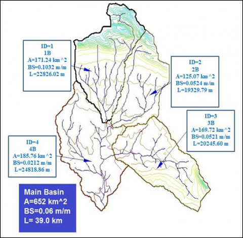
AL-Khoser watershed is located about 50 km north-east of Nineveh Governorate, Iraq. The watershed has an area of 652 km2 with about 39 km of length. The main channel from the upstream boundary to outlet has slope of 0.06 m/m. The elevations range between 250 m and 1233 m above mean sea level. Geographically it is bounded by the grid line of 36° 50´ on the north, 36°27´23" on the south, 43° 25´ on the east, and 43° 05 on the west [45].
2.1 Data
In order to develop HEC-HMS model, the required data to estimate the direct runoff hydrograph must be prepared, which includes: map of land use-cover, soil type, and data of observed hydrograph in addition to the rainfall data.
Digital elevation Model (DEM) of the study area with resolution (30m×30m) in addition to Watershed Modeling System (WMS) was used to estimate the elevation and slope and other characteristics of AL-Khoser watershed. The DEM is prepared by the institutions that manufactured it and is usually with a certain resolution.
The available observed hydrograph data of season 2003-2004, which recorded by Mohammad [45], were used for calibration process of the HEC-HMS model and adjustment of the input data [45]. Table 1 indicates the available observed hydrographs data of AL-Khoser watershed.
Table 1. Summary of available observed data of season 2003-2004 at the AL-Khoser watershed, measured by Mohammad [45]
|
Rainstorm No. |
Rainfall Depth (mm) |
Intensity mm/hr |
Peak Runoff (m3/sec) |
Peak Sediment (Kg/m3) |
|
I |
19 |
0.8-0.9 |
32 |
2.6 |
|
II |
18 |
2.0-3.5 |
51 |
3.2 |
|
III |
19 |
6.0-9.0 |
66 |
3.6 |
|
IV |
9 |
8.8 |
4.7 |
0.8 |
|
V |
17 |
1.2-2.8 |
54 |
3.2 |
2.2 Land use-land covers and soil map
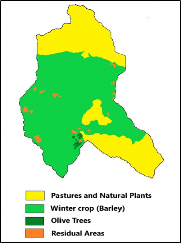
Land use-land cover map of AL-Khoser watershed was derived by Mohammad [45] based on the map of land use-land cover for Nineveh Governorate produced by Remote Sensing Center, University of Mosul [46]. Land use-land cover map were enhanced and used by Younes [47] as shown in Figure 1.
AL-Khoser watershed is part of semi-arid region. About third of its area is bare soil throughout the year due to a high infiltration rate, in addition, presence of steep hills especially at north and east part [45], the remaining is a good rain-fed land. Considering land use, this land is often used for Barley, which is the most important traditional agriculture crops in the area due to drought tolerance, in addition pasture and seasonal grass. Wheat is not considered for this study, however, it may be used with limited area for good rainfall condition season.
Farmers villages with a limited population are also available inside the AL-Khoser watershed that covered about 8.29 km2, Olive trees with limited area of about 3.6 km2 [47].
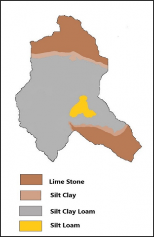
Mainly the watershed has three soil types which are silt clay loam, silt clay, and silt loam [45].
Soil type map was enhanced and used by Younes [47] as shown in Figure 2.
Data of soil type, samples locations, and laboratory tests including: sieve analysis of soil samples and hydrometer test were obtained from previous study [45].
Figure 1. Land use map of AL-Khoser watershed
Figure 2. Soil type map of AL-Khoser watershed
In this study, the land use refers to current land use.
Land use in any area has a significant impact on the watersheds in general and directly affects the change in hydrological conditions and the amount of loss in excess rainfall, and thus the amount of runoff resulting from the watersheds.
The use of land in the AL-Khoser watershed has been almost unchanged over the decades because it is a remote rural area with a rainfed agricultural lands. The only major change may be the construction of a few scattered rural houses in small areas distributed throughout the area of AL-Khoser watershed.
The geological investigation for AL-Khoser catchment area that made by Iraqi Ministry of Irrigation in cooperation with the consultant SOGREAH, French company [48], showed that, the subsurface soil of the AL-Khoser watershed consists of a layer with a thickness of 9-18 (m) of clay soil or silty clay over a strong impermeable layer of silty marls and marls which extends to a depth of 36 (m). These two layers are characterized by low permeability and high bearing capacity. Natural raw soil materials for construction dam body are available in AL-Khoser watershed.
2.3 Rainfall
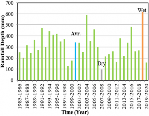
The rainfall of the meteorological Mosul station - Iraqi Department of Meteorology and Seismic Monitoring was considered for the period 1985-2020.
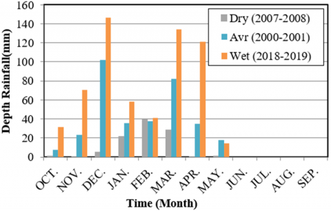
The rainy seasons were classified into three seasons: dry, average, and wet, based on the minimum, average, and maximum total annual rainfall (Figure 3). Monthly rainfall of these three rainfall seasons were presented in Figure 4.
The rainfall in the study area is distributed with low depth and fluctuating value. Dry season is the rainfall season which has a minimum depth of rainfall during the study period, which was achieved during the season (2007-2008) with total annual rainfall depth of 97 mm, while the average season is the rainfall season that has a depth of rainfall in between the minimum and maximum rainfall depths during the study period (arithmetic average of rainy season depths), which was achieved during the season (2000-2001) with total annual rainfall depth of (342) mm, and the wet season is the rainfall season that has maximum depth of rainfall during the study period, which was achieved during the season of (2018-2019) with total annual rainfall depth of (618) (mm).
Figure 3. Rainfall distribution for the study period
Figure 4. Monthly rainfall of dry, average, and wet season
The complicated process of operating a reservoir requires the availability of a dataset and different types of models including: using Digital Elevation Model (DEM) with the Watershed Modelling System (WMS) for determining the suitable locations of rainwater harvesting (RWH) dams and the capacity of these reservoirs. Then the Hydrologic Engineering Center-Hydrologic Modeling System (HEC-HMS) V. 4.2 was used to determine the volume of harvested water for the reservoirs individually based on soil conservation service curve number (SCS-CN) method. The dead storage for individual reservoir was determined based on Universal Soil Loss Equation (USLE) and Trap efficiency (Te). Irrigation Water Requirement Model (IWR) was estimated by the differences between consumptives use and effective rainfall based on FAO-56. Maximized total hydropower generation during total time of reservoir operation was done after using a specific technique that used to convert non-linear hydropower generation problems to linear problems, and then Linear Programming was used for single and multi-reservoirs systems based on MATLAB software V. 17a.
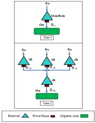
3.1 Cases and Scenarios
This study included two cases, Case 1 is consisted of one Scenario, deals with main basin of AL-Khoser watershed as one unit. While, Case 2 consisted of two Scenarios that deals with a selected four sub-basins inside AL-Khoser main basin, in Scenario 1, the four reservoirs were operated as individual storage systems. The goal is to maximize the hydropower generation for the dry, average, and wet seasons. The outflows from reservoirs 1B, 2B, and 3B were representing an inflow to the reservoir 4B that is located downstream of the above three reservoirs; additional inflow to the reservoir 4B was produced by the volume of runoff from the catchment area of reservoir 4B. In Scenario 2, the four reservoirs were operated as a single storage system; taking into account that the constraints are the storage of each reservoir. The objective function is to maximize the hydropower generation for the above three seasons.
For Scenarios 1 and 2 of Case 2, during downstream water flow, the secondary losses were neglected because of their small amount.
3.2 Watershed Modeling System
Watershed Modeling System (WMS) V.11 is developed by Aquaveo, which is a complete solution for watershed that can be used for delineation, modeling hydrologic, hydraulic, storm drain and routing the rainfall runoff through GIS-based models [49].
Figure 5. Main basin and sub basin of AL-Khoser watershed
In this study, WMS was applied for AL-Khoser basin using Digital Elevation Model (DEM) of the study area. The outlets locations of AL-Khoser main basin and sub-basins (1B, 2B, 3B, and 4B) were identified (Figure 5). It should be noted that, the main basin and the sub-basin (4B) shared the same outlet locations. Reservoirs will be formed at each outlet as a result of building hypothetical dams of rainwater harvesting (RWH). The hydraulic complexity may appear when the hydraulic network is having multiple reservoirs based on series or parallel connections. Accordingly, the three reservoirs (1B, 2B and 3B) have parallel connections among them, and in same time, having series connections with reservoir (4B) (Figure 6). The engineering characteristics of the RWH dams were estimated (Table 2).
Figure 6. Hydraulic network of AL-Khoser watershed
Table 2. Engineering characteristic of the hypothetical RWH dams
|
Dams Details |
Max Height (m) |
Max Dam Length (km) |
Catchment Area (km2) |
|
Main basin |
12 |
980 |
652.00 |
|
1B |
11 |
480 |
171.24 |
|
2B |
10 |
730 |
125.07 |
|
3B |
10 |
685 |
169.72 |
|
4B |
12 |
980 |
185.76 |
3.3 HEC-HMS model
HEC-HMS is developed by the US Army Corps of Engineers to simulate the hydrologic response of a watershed subject to a given hydro meteorological input [50].
The HEC-HMS model is a physical semi-distributed model, that can simulate the relationship of rainfall-runoff for a wide range of watershed areas. HEC-HMS has included many of the most common methods in hydrologic engineering such as losses, runoff transformation, open channel routing, analysis of meteorological data, rainfall-runoff simulation, and parameter estimation [51].
3.3.1 HEC-HMS project
HEC-HMS project consist of four components: Basin models that represent the physical properties of the watershed, and include hydrologic elements that connected in a dendritic network (Sub-basin, reach, junction, reservoir, diversion, source, and sink) for simulating the water movement of watershed. Meteorological models which help to prepare meteorological boundary conditions for sub basins. Control specifications which are used to control the time interval of simulation, and include a starting date and time, ending date and time, and computation time step. Time-series data, that represent the time-series of precipitation data for estimating basin-average rainfall, observed discharge data included for calibration process [52].
3.3.2 Loss method
Precipitation loss is represented by the SCS-CN method to determine the hydrologic loss rate. The SCS loss model for basin loss is given by:
$Q=\frac{(P t-I a)^2}{(P t-I a+S)}$ (1)
$I a=0.2 S$ (2)
$\begin{gathered}Q=\frac{(P t-0.2 S)^2}{(P t+0.8 S)} \text { for } P t>I a \\ Q=0 \text { for } P t<0.2 S\end{gathered}$ (3)
where, Q=accumulated precipitation excess at time t, Pt=accumulated rainfall depth at time t; Ia=initial abstraction or Initial Loss; S=potential maximum retention after runoff begins; Q, P, and S have length units.
$S=\frac{2540}{CN}-25.4(SI system)$ (4)
CN is the SCS curve number and it is a dimensionless number based on the area's hydrologic soil group, land use, treatment and hydrologic condition.
3.3.3 Transform method
Transform method (SCS-UH) allows specifying how to convert excess rainfall to direct runoff. SCS-UH is a dimensionless unit hydrograph, expresses the UH discharge, Ut, as a ratio to the UH peak discharge, Up, for any time t, a fraction of Tp, the time to UH peak [52]. The UH peak and time of UH peak are related by:
$U P=C c *\left(\frac{A 1}{T P}\right)$ (5)
$T p=\frac{\Delta t}{2}+T_{lag }$ (6)
where, Cc is the conversion constant (2.08 in SI) and A1 is the sub-watershed area, Δt is the time step in HEC-HMS and Tlag is the time lag defined as the time difference between the center of excess precipitation and the center of UH [52].
Lag time (Tlag) of watershed is the time span between the mass of excess rainfall to the peak of hydrograph. Time of concentration (Tc) is the time required for runoff to travel from the hydraulically most remote point of the watershed to the outlet. In hydrograph analysis, time of concentration is the time from the end of excess rainfall to the point on the falling limb of the hydrograph (point of inflection) where the recession curve begins [53].
$T_{lag}=L^{0.8}\left[\frac{(S+L)^{0.7}}{1900 Y^{0.5}}\right]$ (7)
Mockus [54] and Simas [55] found that for average natural watershed conditions and approximately uniform distribution of runoff lag time may expressed as:
$T_{lag}=0.6 T_c$ (8)
Applying Eq. (8) in Eq. (7) leads to:
$T_c=L^{0.8}\left[\frac{(S+L)^{0.7}}{1140 Y^{0.5}}\right]$ (9)
where, Tlag=lag time, h; Tc=time of concentration, h; (Tc) was developed by the Soil Conservation Service (SCS); L=flow length, ft; Y=average watershed land slope, percent.
The Tc of SCS model, in SI unit, may be expressed as:
$T_c=227 * L m^{0.8}\left[\frac{(S+L m)^{0.7}}{\left(105 * Y^{0.5}\right)}\right]$ (10)
where, Tc in hr; Lm=flow length (m).
3.3.4 SCS hypothetical storms
Soil Conservation Service developed hypothetical storms (SCS Storms) as averages of rainfall patterns; they are represented in a dimensionless form. The intended use is for estimating both peak flow rate and runoff volume from precipitation of a "critical" duration. Four different storm patterns were developed for a small drainage area at United States [56]. The so-called Type I storm represents areas of climates with generally wet winters and dry summers [52]. In this study SCS Storms Type (I) was used.
3.4 Dead storage model
One of the major problems that are facing dams’ reservoirs is sedimentation, the negative impact of the sedimentation may be represented mainly by reducing the storage capacity and life span of the reservoirs and then the operation efficiency, therefore, during planning of reservoir project a provision is made for a certain storage capacity, specifically for sediment deposition, called dead storage [57]. The sediment deposition is mainly formed by the annual sediment inflow (As) in (MCM) (Eq. (11)):
$A s=A s p * A c$ (11)
$A s p=\left(\frac{A}{S w}\right)$ (12)
where, Asp=Annual sediment production (m3/km2); Ac=catchment area (km2); A=average annual soil loss in tons per hectare per year; Sw=Specific weight of the sediment (gm/cm3).
Part of Asp is trapped in the reservoir, depends upon the average trap efficiency (Te) during each year, and this trap efficiency, in turn, depends upon the capacity/inflow ratio (C/I) (Table 3).
Table 3. Te for capacity/inflow ratio (C/I) [57]
|
C/I |
0.01 |
0.02 |
0.04 |
0.06 |
0.08 |
|
Te % |
43 |
60 |
74 |
80 |
84 |
|
C/I |
0.1 |
0.2 |
0.3 |
0.5 |
0.7 |
|
Te % |
87 |
93 |
95 |
96 |
97 |
The modeling of sedimentation is based on the Universal Soil Loss Equation (USLE) that was developed by Wischmeier and Smith [58], where the average annual soil loss (A) may be expressed as:
$A=K * L C * P * L S * R$ (13)
where, K=soil erodibility coefficient; LC=land cover factor; P=support practices; LS=slope length - slope gradient factor. Rainfall erosivity factor (R) can be estimated using monthly and annual precipitation (pi and p) respectively by Eq. (14):
$\log R=1.93 \log \sum \frac{P_i^2}{P}-1.52$ (14)
The slope length - slope gradient (LS) can be found by Eq. (15):
$L S=[0.065+0.0456($ slope $)+0.006541($ slope $)] *(\text { slope length } / \text { constant })^{N N}$ (15)
where, slope=slope steepness in %; slope length=length of slope in (m); constant=22.1 (SI unite); NN=the exponent value of the equation value (15) depends on the slope (Table 4).
Table 4. NN values
|
S |
˂ 1 |
1 ≤ Slope ˂ 3 |
3 ≤ Slope ˂5 |
≥ 5 |
|
NN |
0.2 |
0.3 |
0.4 |
0.5 |
Based on the data of the study area, it was imposed that the probable life of the RWH reservoirs is 25 years. The probable life of the reservoir is calculated when capacity is reduced by 10% of its initial capacity by sedimentation that forming the interval volume Eq. (16):
Interval Volume $=10 \% * C$ (16)
where, C=storage capacity of reservoir (MCM).
The required time for the interval volume calculation is based on the average Te, the average of Te is calculated based on the start and the end of the Interval Volume, so the annual sediment load (MCM / yr) may give by Eq. (17):
$S l=A s *$ Average trap efficiency $T e$ (17)
where, Sl=annual sediment load (MCM / yr).
years No. of the interval volume $=10 \% *\left(\frac{S c}{S l}\right)$ (18)
In case, the result of Eq. (18) is equal or greater than the probable life of the reservoir, this means that the sediment volume=the result of Eq. (17) multiplied by the probable life of the reservoir; which gives the dead storage.
In case, the result of Eq. (18) is less than the probable life of the reservoir, the solution will need to increase Interval Volume to 20% (increased by a new 10%) and then to repeat the above calculation and so on till the result of Eq. (18) is equal or greater than the probable life of the reservoir.
3.5 IWR model
In this model, FAO Irrigation and Drainage paper 56 [59] was considered to estimate the IWR (the needed water to be supplied to the crop of the rain-fed agriculture land) as follows: The consumptive use for the considered crop (CUi) For each time interval (i) was estimated by the following equation:
$C U_i=E T_i^o * K c_i$ (19)
where, EToi=reference crop evapotranspiration at interval (i) (mm); Kci=crop coefficient at interval (i).
The needed irrigation depth (NIDi) for each time interval (i) was estimated by the following equation:
$N I D_i=C U_i-$ depth of effective rainfalli for $C U_i>$ depth of effective rainfall$_i$ (20)
$N I D_i=$ zero for $C U_i \leq$ depth of effective rainfall ${ }_i$ (21)
$v w_t=\sum N I D_i * 10^{-2}$ (22)
$V w_t=v w_t * a$ (23)
where, vwt=volume of irrigation water requirement monthly per hectare (MCM/m/hec.); t=time period by month; Vwt=volume of irrigation water requirement monthly (MCM); a=irrigation area (hec.).
3.6 Optimized hydropower operation model
Optimization models are among the mathematical models through which water storage systems can be represented. The optimization model can deal with the system's physical variables through mathematical equations that express the potential of that system and its limitations. The equations of these models are solved using several programs and techniques, such as linear, non-linear programming, genetic algorithms, and other programs and techniques that have been explained in previous studies.
In this study, optimized hydropower operation model (OHOM) was proposed to express storage systems when the main goal is to generate hydropower, where the production of hydropower during any period of any reservoir depends on the capacity of the installed plant, flow through the turbine, the average effective productive storage head, number of hours in a period (fraction of time in which energy is produced), The plant factor which is a constant for converting the output of plant efficiency, flow and head into electrical energy in units of kilowatt-hours (KWhi) that produced in period i.
The objective function is to maximize the total hydropower generation during the total operating time of the reservoir and is expressed mathematically as in literatures [60-62] as follows:
$E=\sum_i^n K h * R_i * H_i * \mathrm{\eta}$ (24)
where, E=total hydropower generation during total time of reservoir operation, kWh; Kh=constant to convert the hydropower to (kWh); Ri=Average release for hydropower during time (i); Hi=average of water elevation in the reservoir from the turbine in time (i); ŋ=hydropower plant operation efficiency, which was hypothesized to be constant.
It is clear that the hydropower generation equation is a non-linear type and complicated due to conflicts between variables. For example, if we want to increase hydropower generation by increasing releases (R), then this process will be useless if not carefully studied the situation, because increasing the release will be accompanied by decrease in the water column (H), which is the second variable on which hydropower generation equation depends. The opposite is true, so it is unlikely to increase energy for the above situation. For these reasons, the OHOM model was developed, has the ability to simplify and solve the complexity and conflict of non-linear problems by making some assumptions and then using linear programming (LP) solutions (mathematical model which is a special case of mathematical programming) to arrive to the optimal result (maximizing hydropower generation).
OHOM model presents an application of linear programming formulation for the operation of a single and multi-reservoirs for generating hydropower based on MATLAB software.
A linear approximation of the non-linear power production term [60] is used followingly. The non-linear power production term is the vectors of the flow (R), and the head (H). For example, it may be linearized by the approximation [61] as follows:
$R. H=R_1 * H_1+R_2 * H_2+\ldots+R_n * H_n$ (25)
where, the nonlinear Eq. (24) can be replaced with the linear Eq. (26) as an objective function Z for maximizing hydropower generation. Eq. (26) linearly sums up each element of R and H. since the storage water level Hi is directly proportional to the storage volume Si [40].
$\operatorname{Max} Z=C 1 \sum_{i=1}^n R_i+C 2 \sum_{i=1}^n S_i$ (26)
where, C1 and C2 are the parameters values of release and storage for the vectors R, and S respectively.
This model subjects to specific constraints of system’s components. In the following, the optimization models are presented for a single and multi-reservoirs.
Where the complex and conflict non-linear problems can be simplified and solved by making a few assumptions for the objective function and constraints, then use Linear Programming (LP). The non-linear power production term is the vector multiplication of the vectors (the release, and the head). In which a linear approximation of the non-linear power production term can be expressed linearly by summing the vectors (the release, and the storage). where the relationship between the head and the storage is directly proportional. hence maximum head is achieved when maximum storage is reached. Therefore, the vectors of the non-linear objective function of power production were obtained by using linear objective function.
3.6.1 Single reservoir operation (SRO)
For the SRO, the needed objective function will be as follows:
$\operatorname{Max} Z=C 1 \sum_{i=1}^{12} R_i+C 2 \sum_{i=1}^{12} S_i$ (27)
Through the above equation, the maximum release of water is found while maintaining the maximum storage (the two basic variables of the hydroelectric energy equation).
The above objective function is subjected to the constraints of water balance equation and its components.
The continuity equation represents the most important physical constraints of the mathematical model, which links the input and output variables of the reservoir. The continuity equation is the amount of balance between the contents of the reservoir from the beginning (Si) to the end of the period (Si+1) including the surface runoff (Rni), resulting from rainfall and will be calculated using the HEC-HMS model, evaporation (Ei) from reservoir, and releases (Ri) can be expressed by the following mathematical formula.
$S_{i+1}=S_i+R n_i-R_i-E_i$ (28)
The minimum and maximum limitation of storage constraint are represented by the reservoir dead storage and the maximum reservoir capacity where they are calculated by the dead storage model and WMS program respectively.
$S_{\text {min }} \leq S_i \leq S_{\text {max }}$ (29)
The minimum and maximum limitation of water release constraints are represented by the irrigation water demand and the maximum release through hydropower outlets where they are calculated by the IWR model and the hydropower outlets capacity that are determined by the type of turbines used respectively.
$R_{\text {min }} \leq R_i \leq R_{\text {max }}$ (30)
The limit of the total water release constraint must not exceed the total annual surface runoff entering the reservoir during the year, described as follows:
$\sum_{i=1}^{12}\left(R_i\right) \leq \sum_{i=1}^{12} R n_i$ (31)
where, Si+1= stands for the volume (MCM) of the water stored in the reservoir at the end of the (i) month; Si=water stored in the reservoir at the beginning of the month; Rni=volume (MCM) of the rainwater that was added to the reservoir during the month (i); Ei=the average volume (MCM) of water loss due to evaporation from the surface of the reservoir during the month (i); Smin=minimum operational storage (MCM); Smax=maximum operational storage (MCM); Rmin=minimum release, which represents the monthly water supplies (MCM) for the irrigated area downstream the reservoir during the month (i); and Rmax=stands for the maximum release (MCM) from the outlets of hydropower generation during the month (i).
3.6.2 Multi-reservoir operation
For the multi-reservoir operation (MRO), the needed objective function will be as follows:
$\operatorname{Max} Z=\sum_j^4\left(C 1 \sum_{i=1}^{12} R_{j i}+C 2 \sum_{i=1}^{12} S_{j i}\right)$ (32)
Through the above equation, the maximum release of water is found while maintaining the maximum storage (the two basic variables of the hydroelectric energy equation) for the four reservoirs in same time.
Eq. (32) is subjected to the following constraint:
The constraint of the continuity equation for each of the three reservoirs B1, B2, and B3 including: each reservoir depends on the storage at the beginning and end of the period, the associated runoff, the evaporation resulting from it, and the releases of water allocated for irrigation required from it.
$S_{j(i+1)}=S_{j i}+R n_{j i}-R_{j i}-E_{j i}$ (33)
The constraint of continuity equation for reservoir B4 resulting from the method of connecting the four reservoirs explained previously depends on the storage at the beginning and end of the period, its affiliated runoff, the releases coming to it from the three tanks above it, the evaporation resulting from it, and the irrigation releases required to be provided from it.
$S_{j(i+1)}=S_{j i}+R n_{j i}+R_{1 i}+R_{2 i}+R_{3 i}-R_{j i}-E_{j i}$ (34)
The storage constraint for each of the four reservoirs can be explained as follows: for each reservoir, the storage must not be less than the dead storage and not exceed the storage capacity.
$S_{\text {jmin }} \leq S_{j i} \leq S_{\text {jmax }}$ (35)
The water release constraint for each of the four reservoirs explained by: for each reservoir, the water release must not be less than the IWR and not exceed the hydropower outlets capacity.
$R_{\text {jmin }} \leq R_{j i} \leq R_{\text {jmax }}$ (36)
The constraint of total water release for the four reservoirs must not exceed the total annual surface runoff entering each reservoir during the year, and it can be described as follows:
$\sum_{i=1}^{12}\left(R_{j i}\right) \leq \sum_j^4\left(\sum_{i=1}^{12} R n_{j i}\right)$ (37)
These models will be applied practically to the AL-Khoser basin for the two cases referred to in Section 3.1 to determine the effectiveness of these models in addressing the problem of hydropower generation in the Al- Khoser basin and to clarify the benefit resulting from each case in order to come up with a decision that expresses the best case that would prefer to be adopted.
Quantitative analysis was used which included mathematical modeling (in most of this study) and statistical modeling (in HEC-HMS model performance) in terms of numerical values to understand rainwater harvesting and objective function of hydropower generation.
The relationships between storage-elevation and storage-area for each reservoir were estimated using WMS. Storage capacity of each reservoir was estimated too (Figure 7).
In this study, the calibration process of HEC-HMS (Figure 8) showed a reasonable fit between simulated and observed hydrograph shapes, the observed hydrograph was recorded by Mohammad [45] and fixed for constant interval time, the statistical tests of HEC-HMS evaluation results and its performance gave encouraging results to increase confidence in the results of the HEC-HMS model. Where calculated Peake discharge= 44.0 m3/sec, while observed Peake discharge=51.0 m3/sec. The simulated discharge hydrograph that obtained by HEC-HMS model is reasonably and acceptably matched with the observed discharge hydrograph with NashSutcliffe efficiency (NSE) [63] of 85.7%, Mean Abs. Error (MAE) and Root Mean Squared Error (RMSE) of 4.8 and 3.0 m3/s respectively.
Figure 7. Storage capacity for the selected reservoirs
Figure 8. HEC-HMS model calibration
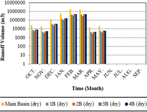
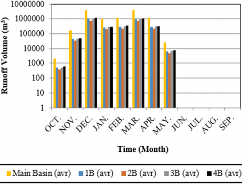
Table 5. Annual harvested water (MCM) for the selected three season
|
Season |
Main Basin |
1B |
2B |
3B |
4B |
|
Dry |
4.1788 |
1.0744 |
0.7790 |
1.1132 |
1.2118 |
|
Average |
11.4010 |
2.9315 |
2.1256 |
3.0372 |
3.3062 |
|
Wet |
28.1985 |
7.2771 |
5.10158 |
7.5149 |
8.1815 |
(a)
(b)
(c)
Figure 9. (a) Estimated monthly harvested water for the dry season; (b) Estimated monthly harvested water for the average season; (c) Estimated monthly harvested water for the wet season
And then, HEC-HMS was applied, using daily rainfall data of the selected three seasons (dry, average, and wet) to estimate the monthly harvested water (Figures 9). The annual harvested water (MCM) for the selected three seasons is presented in Table 5.
The results demonstrate the success of the rainwater harvesting system for collecting the harvested water in reservoirs, creating a new water source. The volumes of runoff were calculated using HEC-HMS. These volumes were resulting by individual daily rain storm throughout the selected rainy seasons of dry, average, and wet season.
Estimating the volume of harvested rainwater included the same two cases that mentioned in methodology. Case 1 deals with main basin of AL-Khoser watershed as one unit. While, Case 2 deals with selected four sub-basins inside AL-Khoser main basin. The runoff volumes (harvested water) represented monthly as shown in the Figure 9 by reservoir 1B, 2B, 3B, 4B and main basin for the seasons mentioned above. In order to give a more comprehensive idea about the volume of harvested water annually, the results were presented in Table 5.
The results indicate that in the dry season, despite the limited rainfall, the volume of water harvested ranged between 0.779-1.2188 (MCM) through the reservoirs 1B to 4B, while the volume of water harvested from Al-Koser watershed reached up to 4.178 (MCM) as one main basin.
During the average rainy season, where the amounts of rainfall increased, the volume of water harvested annually ranged between 2.1256 - 3.0372 (MCM) for the four reservoirs (B1 to B4), while the volume of water harvested from Al-Koser watershed reached up to 11.401 (MCM) as one main basin. More harvested water is available during wet season that ranged between 5.10158 - 8.1815 (MCM) for the four reservoirs (B1 to B4), while the volume of water harvested from Al-Koser watershed reached up to 28.1985 (MCM) as one main basin.
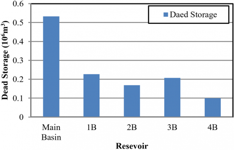
The volume of sediments of each reservoir has been estimated by running the dead storage model based on the results of the runoff volume of average season, storage capacity and the imposed probable life (25 years) of each reservoir. Observing Figure 10 shows that the volume of dead storage reached 0.1 (MCM) for the B4 reservoir, while it reached 0.533 (MCM) for the main basin reservoir, knowing that the two reservoirs mentioned above share the same outlet.
Figure 10. Volume of dead storage of each selected reservoir
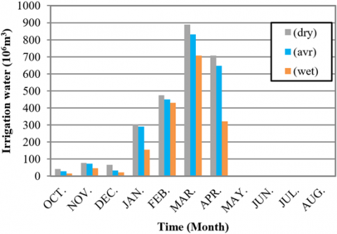
Figure 11. Results of the monthly irrigation requirements for each hectare for the (dry, average and wet) seasons
The reason for the decrease in dead storage in the B4 reservoir can be attributed to the presence of the three reservoirs that are located at the Upstream of B4 reservoir, which will work to trap sediments and prevent them from reaching the B4 reservoir. Figure 10 shows the volume of dead storage of each selected reservoir.
The lands of AL-Khoser watershed are famous for rain-fed agriculture with the national income of crops, barley, which is the most important traditional agriculture crops in the area due to drought tolerance. For this study, Barley was chosen as the agricultural crop. Figure 11 shows the results of the monthly irrigation requirements for each hectare for the three seasons (dry, average and wet).
For Case 1, in order to estimate the total hydropower, SRO model was applied with Main Basin, for dry, average and wet seasons; the total numbers of the model variables were 48.
The sensitivity analysis was applied for the parameters values (C1 and C2). The analysis was considered for all reservoirs and for the three selected seasons. For example, Table 6, shows the values of C1 and C2 for reservoir main basin during the wet season.
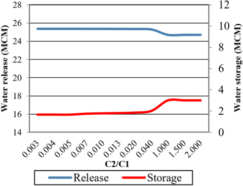
Table 6. Annual results of the hydropower for main basin during wet season according to sensitivity parameters
|
C1 |
C2 |
C2/C1 |
R (MCM) |
P (KW) |
|
500 |
1 |
0.0020 |
25.34 |
658.68 |
|
400 |
1 |
0.0025 |
25.34 |
658.68 |
|
350 |
1 |
0.0028 |
25.34 |
658.68 |
|
250 |
1 |
0.0040 |
25.34 |
658.68 |
|
200 |
1 |
0.0050 |
25.34 |
658.68 |
|
150 |
1 |
0.0066 |
25.34 |
659.44 |
|
100 |
1 |
0.0100 |
25.33 |
665.71 |
|
75 |
1 |
0.0133 |
25.33 |
668.87 |
|
50 |
1 |
0.0200 |
25.32 |
672.13 |
|
25 |
1 |
0.0400 |
25.27 |
675.73 |
|
1 |
1 |
1.0000 |
24.69 |
730.61 |
|
1 |
25 |
25.000 |
24.69 |
730.61 |
|
1 |
50 |
50.000 |
24.69 |
730.61 |
|
1 |
75 |
75.000 |
24.69 |
730.61 |
|
1 |
100 |
100.00 |
24.69 |
730.61 |
|
1 |
500 |
500.00 |
24.69 |
730.61 |
Figure 12. Annual hydropower for main basin during wet season according to the sensitivity parameters
Figure 13. Relationship between the water release and water storage
The selected values of C1 and C2 were based on maximum hydropower generated [40]. The results of the analysis show that the highest value of energy generation is 730.61 KW when the values of both C1 and C2 are equal to 1. When the values of C2 are greater than 1, the generated hydroelectric energy values do not improve as shown in Figure 12, which shows the annual hydropower for main basin during wet season according to the sensitivity criteria. The relationship between the water release and water storage for given C2/C1 is shown in Figure 13.
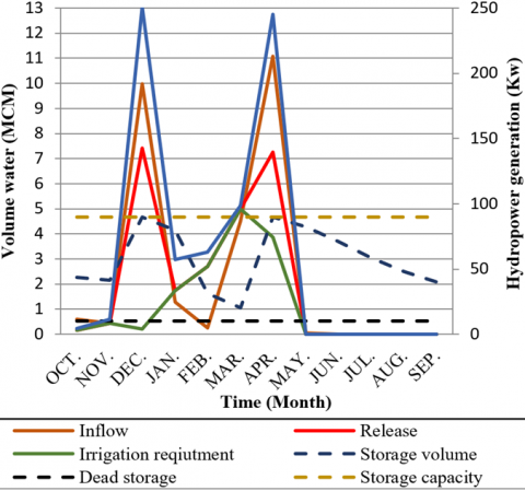
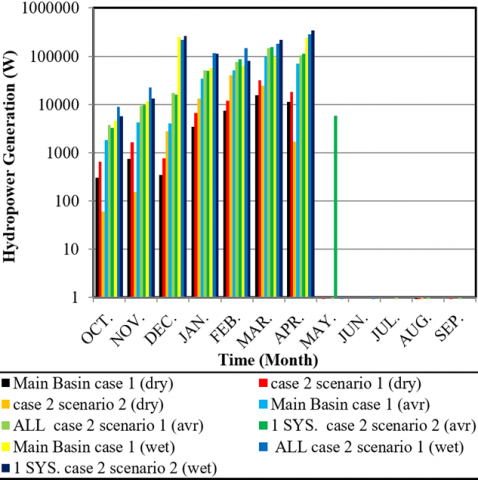
The maximum monthly operating policy for the SRO model is shown in Figure 14, that shows the inflow water volume, irrigation requirement, storage volume in the reservoir (S), maximum releases (R), and the amount of hydropower generation.
Figure 14. Results of optimal reservoir operation for main basin during wet season as calculated by the SRO model
According to the applicable priority level. The releases (R) meet irrigation requitement with the lowest priority, and they provide the highest hydropower generation.
It is clear that the maximizing hydropower generation with a high storage level did not reduce the release of irrigation requirement during the maximum monthly operating policy of SRO model.
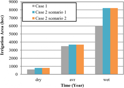
The results of maximum generated hydropower were 39.02, 263.49, and 730.61 (Kw/year) for the selected three seasons (gray color of Figure 15). The irrigation areas were identified previously (600, 3500, and 6000) hectare/year, as the constraints, for the same above seasons respectively (gray color of Figure 16).
For Case 2, at the beginning, Scenario 1 was used by applying SRO with 1B, 2B, and 3B and then, the reservoirs releases were added in water balance equation of SRO when applied with reservoir 4B for dry, average and wet season. The total numbers of the SRO model variables were 48. The results of maximum generated hydropower were 72.122, 408.55 and 975.07 (Kw/year) for the selected three seasons (blue color of Figure 15). The irrigation areas were identified previously (800, 3675, and 8220) hectare/year, as the constraints, for the same above seasons respectively (blue color of Figure 16).
The results of Scenario 1 of Case 2 show that, there was an increase in generated hydropower for each season (dry, average, and wet) compared with Case 1, where the increased ratio reached about 85, 55, and 33.5 (%) respectively (Figure 15, blue color).
Once again, it should be noted that the main basin and the sub-basin (4B) shared same outlet locations.
The reasons of increased generated hydropower were due to two reasons, the first, is same water that released from 1B, 2B, and 3B, was reused in 4B, the second, is that the storage capacity of reservoir 4B became greater than the storage capacity of main basin reservoir, as the volume of dead storage of reservoir 4B decreased due to the presence of reservoirs 1B, 2B, and 3B, which lead to the turbine level of reservoir 4B being lower than the turbine level of main basin reservoir, thus obtaining a higher water column height.
Figure 15. Annual power generation for Case 1 (gray color), Case 2-Scenario 1 (blue color), and Case 2-Scenario 2 (orange color)
Figure 16. Annual irrigation area for Case 1 (gray color), Case 2-Scenario1 (blue color), and Case 2-Scenario 2 (orange color)
The irrigation areas of Scenario 1 were increased compared with Case 1, by 37, 10, and 34 (%) for dry, average and wet seasons respectively (blue color of Figure 16) due to the two reasons mentioned above, in addition to the volume distribution of surface runoff in the rainy season, it also has an impact on the size of irrigated areas. The reason is due to the fact that rainstorms may occur in successive short periods of time, which will fill the reservoir )preferred), or may be distributed in spaced periods during the season. Where it can be noted that the percentage of increase in irrigation areas is not regular in a fixed amount for the three selected seasons; although the total irrigation areas in the dry season were less than that of the average and wet seasons.
In Scenario 2 of Case 2, the four reservoirs were operated as a single storage system taking into account that the storage of each reservoir is a constraint of the problem to keep the objective function which is maximizing the generation of hydropower for the three selected seasons. The MRO model was applied to the four reservoirs, the number of variables was 72, same constraints of irrigation requirement that applied in Scenario 1 were used, this means using the same values of irrigated areas that applied in the Scenario 1 (Figure 16, orange color); this is to obtain maximized hydropower generation without the releases being affected by irrigation requirements; by this the difference in energy becomes clear between Scenarios 1 and 2.
The results of Scenario 2 explained that the capacity of generation was 82.59, 436.75, 1034.70 kW for the three selected seasons respectively. Also, the results of Scenario 2 showed that there was a percentage increase in hydropower generation over Scenario 1 which reached 14.5, 7, and 6 (%). And that the percentage increase in hydropower generation over Case 1 which reached 111.60, 65.76, and 41.62 (%) (Figure 15). This increase is due to the previous reasons mentioned in Scenario 1, in addition to that, in Scenario 2, reservoir 4B will receive and store water from sub-reservoirs 1B, 2B, and 3B, and that all requirements are met where is carried out through reservoir 4B. In other words, the three reservoirs generate hydropower without binding constraints to meet the requirements of each reservoir, so the stored water is released from the three reservoirs to reservoir 4B, through which hydropower is generated and all downstream requirements are met.
This procedure gives comfort to the reservoirs 1B, 2B, and 3B and leads to keeping the reservoirs at the highest storage and for the longest possible period, taking into account the minimum values of the surface areas of the reservoirs to reduce evaporation losses optimally.
From the foregoing, it is clear that, Scenario 2 in the Case 2 gave results for generating energy significantly superior from the Case 1, at the same time, the irrigated areas were increased.
Figure 17 shows the values of monthly hydropower generation that can be generated in the three seasons for the Case 1 and for the Scenarios 1 and 2 of the Case 2.
Figure 17. Monthly hydropower generation for the three seasons of Case 1 and for the Scenarios 1 and 2 of Case 2
Figure 18. Monthly irrigation requirements for the three seasons of Case 1 and Case 2
Figure 18 shows the monthly irrigation requirements for the three seasons of the Case 1 and Case 2.
As a summary RWH can provide a new water source that can be used for irrigation and hydroelectric power generation. The maximum harvested water reached 28.1985 (MCM) during the study period (1985-2020).
Dividing the main basin into four sub-basins does not lead to an increase in the volume of harvested water, but it achieves benefits in the following areas: trapping sediments and preventing them reaching the reservoir of the outlet, which leads to an increase in its capacity, and also leads to an increase in both hydropower generation and irrigated areas, where the maximum hydropower generation and maximum irrigated areas have been reached 1034 (Kw) and 8220 (hec).
Rainwater harvesting system is a key solution to address the shortage of water requirements for agriculture and electric power for remote rural communities in arid and semi-arid regions such as AL-Khoser watershed, Iraq.
The results showed that, by using HEC-HMS model, the annual harvested water in the selected reservoirs Main Basin, 1B, 2B, 3B and 4B ranged between: 0.7790-4.1788, 2.1256-11.4010, and 5.10158-28.1985 MCM for dry, average and wet season respectively.
Encouraging results for seasonal Scenarios show that rainwater harvesting may reduce water scarcity even during dry seasons.
OHOM was developed to convert non-linear problems to linear ones. Two models were developed and used for maximized annual hydropower generation, the first single-reservoir operation (SRO) and the second, multi-reservoir operation (MRO).
Three rainy seasons (dry, average, and wet) were adopted throughout the study period (1985-2020).
The results of generating hydropower for single reservoir of rainwater harvesting system (Case 1) are as follows: 39.02, 263.49, 730.61 Kw for the selected seasons respectively.
The results of generating hydropower for multi-reservoir of rainwater harvesting system (Case 2 Scenario 1) are as follows: 72.122, 408.55, 975.07 Kw for the selected seasons respectively.
The results of generating hydropower for multi-reservoir of rainwater harvesting system (Case 2 Scenario 2) are as follow: 82.59, 436.75, 1034.70 kW for the selected seasons respectively.
The results of generating hydropower for single and multi-reservoir of rainwater harvesting systems show that there was an increase in hydropower generation achieved through multi-reservoir operation policies (Case 2 Scenario 2) and the results of the hydropower generation comparison for dry, average and wet seasons showed that there was an increase in power generation from Scenario 1 by (15, 7 and 6) % respectively, while the increase over the results of Case 1 reached up to (110, 66 and 41) % respectively.
The irrigated areas for Case 1 were determined as 600, 3500, and 6000 (ha). The irrigated areas for Case 2 were determined as 800, 3675, and 8220 (ha). Both Scenarios 1 and 2 of Case 2 have same constraints of irrigation requirement.
The irrigated areas for Case 2 were increased compared with Case 1, by 33, 10, and 37 (%) for dry, average and wet seasons.
These findings have the potential to greatly enhance the availability of clean, renewable energy in rural areas, contributing to sustainable rural development. The optimization results validated the proposed models.
However, the limitations of such studies may be clarified in two directions: the first is the hydrological condition, the availability of rainfall, which essentially govern the availability of water provision in the arid and semi-arid region. The second is successful rainwater harvesting projects is almost probable only with the support of local government policy.
We extend our sincere thanks and appreciation to the University of Mosul and the Deanship of the College of Engineering for sponsoring scientific researches. We would like to express our deepest appreciation to the WMS and HEC-HMS teams.
|
A |
average annual soil loss, tons. hec.-1 y-1 |
|
A1 |
sub-watershed area Km2 |
|
a |
irrigation area, hec. |
|
Ac |
catchment area km2 |
|
As |
annual sediment inflow, MCM |
|
Asp |
annual sediment production, m3.km-2 |
|
LC |
land cover factor |
|
C |
storage capacity, MCM |
|
Cc |
conversion constant (2.08 in SI) |
|
C1 |
parameter of release |
|
C2 |
parameter of storage |
|
CN |
SCS curve number and it is a dimensionless |
|
constant |
constant 22.1, SI unite |
|
CUi |
consumptive use for the considered crop for each time interval i |
|
E |
total hydropower generation during total time of reservoir operation, kWh |
|
Ei |
the average volume of water loss due to evaporation from the surface of the reservoir during the month i, MCM |
|
EToi |
reference crop evapotranspiration at interval i, mm |
|
Kci |
crop coefficient at interval i, mm |
|
Hi |
average of water elevation in the reservoir from the turbine in time i, m |
|
I |
inflow, MCM |
|
Ia |
initial abstraction or Initial Loss, mm |
|
K |
soil erodibility coefficient |
|
Kh |
constant to convert the hydropower to kWh |
|
Lm |
flow length, m |
|
L |
flow length, ft |
|
LS |
slope length - slope gradient factor |
|
NIDi |
needed irrigation depth for each time interval i, mm |
|
NN |
the value depends on the slope |
|
p |
annual precipitation, mm |
|
P |
support practices |
|
Pt |
accumulated rainfall depth at time t, mm |
|
pi |
monthly precipitation, mm |
|
Q |
accumulated precipitation excess at time t |
|
R |
rainfall erosivity factor |
|
Ri |
average release for hydropower during time i, MCM |
|
Rmax |
maximum release during the month i, MCM |
|
Rmin |
minimum release during the month i, MCM |
|
Rni |
volume of rainwater that added to the reservoir during the month, MCM |
|
S |
potential maximum retention after runoff begins, mm |
|
Si |
water stored in the reservoir at the beginning of the month, MCM |
|
Si+1 |
stands for the volume of the water stored in the reservoir at the end of the month, MCM |
|
Sl |
annual sediment load, MCM. yr-1 |
|
slope |
slope steepness, % |
|
slope length |
length of slope, m |
|
Smax |
maximum operational storage, MCM |
|
Smin |
minimum operational storage, MCM |
|
Sw |
specific weight of sediment, gm.cm-3 |
|
t |
time period, month |
|
Tc |
time of concentration, h |
|
Te |
average trap efficiency, |
|
Tlag |
lag time, h |
|
Tp |
time to UH peak, h |
|
vwt |
volume of IWR, MCM.m-1.hec. |
|
Vwt |
monthly volume of IWR, MCM |
|
Y |
average watershed land slope |
|
Z |
maximizing hydropower generation |
|
Δt |
time step in HEC-HMS |
|
ŋ |
power plant operation efficiency, which was hypothesized to be constant |
[1] Al-Ansari, N.A. (2013). Management of water resources in Iraq: Perspectives and prognoses. Engineering, 5(8): 667-684. https://doi.org/10.4236/eng.2013.58080
[2] Al-Khafaji, H. (2018). Electricity generation in Iraq problems and solutions. Al-Bayan Center Studies Series. https://www.bayancenter.org/en/wp-content/uploads/2018/09/786543454657687.pdf.
[3] Mahmood Agha, O.M.A., Khattab, M.A. (2023). The impact of Ilisu Dam on water flow toward Iraq and identifying the optimal operational strategy for Mosul Dam. Sustainable Water Resources Management, 9(4): 112. https://doi.org/10.1007/ s40899-023-00889-0
[4] Boers, T.M., Ben-Asher, J. (1982). A review of rainwater harvesting. Agricultural Water Management, 5(2): 145-158. https://doi.org/10.1016/0378-3774(82)90003-8
[5] Critchley, W., Siegert, K. (1991). Water harvesting for improved agricultural production. Water Report 3, in Proceedings of the FAO (Food and Agricultural Organization of the UN) Expert Consultation, Cairo, Egypt, November, FAO. Rome, Italy. https://edepot.wur.nl/216065.
[6] Raimondi, A., Quinn, R., Abhijith, G.R., Becciu, G., Ostfeld, A. (2023). Rainwater harvesting and treatment: state of the art and perspectives. Water, 15(8): 1518. https://doi.org/10.3390/w15081518
[7] Schild, M., Fleskens, L., Riksen, M., Shadeed, S. (2023). Economic feasibility of rainwater harvesting applications in the west bank, Palestine. Water, 15(6): 1023. https://doi.org/10.3390/w15061023
[8] Al-Ansari, N., Ezz-Aldeen, M., Knutsson, S., Zakaria, S. (2013). Water harvesting and reservoir optimization in selected areas of South Sinjar Mountain, Iraq. Journal of Hydrologic Engineering, 18(12): 1607-1616. http://doi.org/10.1061/(ASCE)HE.1943-5584.0000712
[9] Mahmoud, S.H. (2014). Investigation of rainfall–runoff modeling for Egypt by using remote sensing and GIS integration. Catena, 120: 111-121. https://doi.org/10.1016/j.catena.2014.04.011
[10] Deksissa, T., Trobman, H., Zendehdel, K., Azam, H. (2021). Integrating urban agriculture and stormwater management in a circular economy to enhance ecosystem services: Connecting the dots. Sustainability, 13(15): 8293. https://doi.org/10.3390/su13158293
[11] Penche, C. (1998). Layman's Guidebook on How to Develop a Small Hydro Site. DG XVII, European Commission.
[12] Walczak, N. (2018). Operational evaluation of a small hydropower plant in the context of sustainable development. Water, 10(9): 1114. https://doi.org/10.3390/w10091114
[13] Nouni, M.R., Mullick, S.C., Kandpal, T.C. (2009). Providing electricity access to remote areas in India: Niche areas for decentralized electricity supply. Renewable Energy, 34(2): 430-434. https://doi.org/10.1016/j.renene.2008.05.006
[14] Kucukali, S., Baris, K. (2009). Assessment of small hydropower (SHP) development in Turkey: Laws, regulations and EU policy perspective. Energy policy, 37(10): 3872-3879. https://doi.org/10.1016/j.enpol.2009.06.023
[15] Bracken, L.J., Bulkeley, H.A., Maynard, C.M. (2014). Micro-hydro power in the UK: The role of communities in an emerging energy resource. Energy Policy, 68: 92-101. http://doi.org/10.1016/j.enpol.2013.12.046
[16] Comino, E., Dominici, L., Ambrogio, F., Rosso, M. (2020). Mini-hydro power plant for the improvement of urban water-energy nexus toward sustainability-A case study. Journal of Cleaner Production, 249: 119416. https://doi.org/10.1016/j.jclepro.2019.119416
[17] Date, A., Akbarzadeh, A. (2009). Design and cost analysis of low head simple reaction hydro turbine for remote area power supply. Renewable Energy, 34(2): 409-415. https://doi.org/10.1016/j.renene.2008.05.012
[18] Harlan, T. (2018). Rural utility to low-carbon industry: Small hydropower and the industrialization of renewable energy in China. Geoforum, 95: 59-69. https://doi.org/10.1016/j.geoforum.2018.06.025
[19] Kamran, M., Asghar, R., Mudassar, M., Abid, M.I. (2019). Designing and economic aspects of run-of-canal based micro-hydro system on Balloki-Sulaimanki Link Canal-I for remote villages in Punjab, Pakistan. Renewable Energy, 141: 76-87. https://doi.org/10.1016/j.renene.2019.03.126
[20] Jawahar, C.P., Michael, P.A. (2017). A review on turbines for micro hydro power plant. Renewable and Sustainable Energy Reviews, 72: 882-887. https://doi.org/10.1016/j.rser.2017.01.133
[21] Valipour, M., Sefidkouhi, M.A.G., Eslamian, S. (2015). Surface irrigation simulation models: A review. International Journal of Hydrology Science and Technology, 5(1): 51-70. https://doi.org/10.1504/ijhst.2015.069279
[22] Alshami, A.H., Hussein, H.A. (2021). Feasibility analysis of mini hydropower and thermal power plants at Hindiya barrage in Iraq. Ain Shams Engineering Journal, 12(2): 1513-1521. https://doi.org/10.1016/j.asej.2020.08.034
[23] Khattab,M.A., Al-Mohseen, K.A. (2020). Planning and decision making under uncertainty (Mosul reservoir optimal operating policy - Case study). Al-Rafidain Engineering Journal, 25(1): 85-96.
[24] e Castro, M.S., Sousa, J.C., Saraiva, J.T. (2017). Hydro scheduling optimization considering the impact on market prices and head drop using the linprog function of MATLAB®. In2017 IEEE Manchester PowerTech, Manchester, UK, pp. 1-6. https://doi.org/10.1109/PTC.2017.7980893
[25] Soares, B.R.D.C., De Almeida, K.C. (2019). Piecewise linear approximations of the hydro power producer problem. Congresso Brasileiro de Automática-CBA, 1(1): 653. https://doi.org/10.20906/CBA2022/653
[26] Thaeer Hammid, A., Awad, O.I., Sulaiman, M.H., et al. (2020). A review of optimization algorithms in solving hydro generation scheduling problems. Energies, 13(11): 2787. https://doi.org/10.3390/en131127
[27] Amani, A., Alizadeh, H. (2021). Solving hydropower unit commitment problem using a novel sequential mixed integer linear programming approach. Water Resources Management, 35(6): 1711-1729. https://doi.org/10.1007/s11269-021-02806-6
[28] Córdoba, A.T., del Nozal, Á.R., Reina, D.G., Gata, P.M. (2021). A Genetic algorithm to optimize penstocks for micro-hydro power plants. In 2021 IEEE Congress on Evolutionary Computation (CEC), Kraków, Poland, pp. 49-56. https://doi.org/10.1109/CEC45853.2021.9504994
[29] Mousavi, S.J., Ponnambalam, K., Karray, F. (2005). Reservoir operation using a dynamic programming fuzzy rule–based approach. Water Resources Management, 19: 655-672. https://doi.org/10.1007/s11269-005-3275-3
[30] Aslan, H.K.Y. (2013). Optimization of power output of micro hydro power station using fuzzy logic algorithm. IJTPE International Journal, 5(1): 138-143.
[31] Hammid, A.T., Sulaiman, M.H.B., Kadhim, A.A. (2017). Optimum power production of small hydropower plant (SHP) using firefly algorithm (FA) in himreen lake dam (HLD), eastern Iraq. Research Journal of Applied Sciences, 12(10): 455-466.
[32] Grigoriu, M., Bica, R.D., Popescu, M.C. (2018). Small hydropower plants optimization for equipping and exploitation software application. Procedia Manufacturing, 22: 796-802. https://doi.org/10.1016/j.promfg.2018.03.113
[33] Najarchi, M., Haghverdi, A. (2020). RETRACTED ARTICLE: Application in optimization of multi-reservoir water systems using improving shuffled complex algorithm. SN Applied Sciences, 2(5): 896. https://doi.org/10.1007/s42452-020-2590-x
[34] Nezhad, O.B., Najarchi, M., NajafiZadeh, M.M., Hezaveh, S.M.M. (2018). Developing a shuffled complex evolution algorithm using a differential evolution algorithm for optimizing hydropower reservoir systems. Water Science and Technology: Water Supply, 18(3): 1081-1092. https://doi.org/10.2166/ws.2017.179
[35] Coban, H.H., Sauhats, A. (2022). Optimization tool for small hydropower plant resource planning and development: A case study. Journal of Advanced Research in Natural and Applied Sciences, 8(3): 391-428. https://doi.org/10.28979/jarnas.1083208
[36] Mariño, M.A., Loaiciga, H.A. (1985). Dynamic model for multireservoir operation. Water Resources Research, 21(5): 619-630. https://doi.org/10.1029/wr021i005p00619
[37] Yeh, W.W.G., Becker, L. (1982). Multiobjective analysis of multireservoir operations. Water Resources Research, 18(5): 1326-1336. https://doi.org/10.1029/wr018i005p01326
[38] Wurbs, R.A. (1993). Reservoir-system simulation and optimization models. Journal of Water Resources Planning and Management, 119(4): 455-472. https://doi.org/10.1061/(asce)0733-9496(1993)119:4(455)
[39] Hartmann, T., Schmoller, H.K., Hinuber, G., Haubrich, H.J. (2005). Midterm generation planning in competitive markets for electrical energy and reserve using a linear programming algorithm. In 2005 IEEE Russia Power Tech, St. Petersburg, Russia, pp. 1-5. https://doi.org/10.1109/PTC.2005.4524509
[40] Yoo, J.H. (2009). Maximization of hydropower generation through the application of a linear programming model. Journal of Hydrology, 376(1-2): 182-187. https://doi.org/10.1016/j.jhydrol.2009.07.026
[41] Salami, A.W., Sule, B.F. (2012). Optimal water management modeling for hydropower system on river Niger in Nigeria. Annals of the Faculty of Engineering Hunedoara, 10(1): 185-192.
[42] Clack, C.T.M., Xie, Y., MacDonald, A.E. (2015). Linear programming techniques for developing an optimal electrical system including high-voltage direct-current transmission and storage. International Journal of Electrical Power & Energy Systems, 68: 103-114. https://doi.org/10.1016/j.ijepes.2014.12.049
[43] Belsnes, M.M., Wolfgang, O., Follestad, T., Aasgård, E.K. (2016). Applying successive linear programming for stochastic short-term hydropower optimization. Electric Power Systems Research, 130: 167-180 https://doi.org/10.1016/j.epsr.2015.08.020
[44] Santos, K.V., Finardi, E.C. (2022). Piecewise linear approximations for hydropower production function applied on the hydrothermal unit commitment problem. International Journal of Electrical Power & Energy Systems, 135: 107464. https://doi.org/10.1016/j.ijepes.2021.107464
[45] Mohammad, M.E. (2005). A conceptual model for flow and sediment routing for a watershed northern Iraq. Doctoral dissertation, Doctoral Thesis, University of Mosul, Mosul, Iraq.
[46] Al-Daghastani, H.S. (2008). Land use and land cover map of Ninevah governorate using remote sensing data. Iraqi National Journal of Earth Science, 8(2): 17-26. https://doi.org/10.33899/earth.2008.5479
[47] Younes, S.S. (2017). Effect of variability curve number on peak of hydrograph for Al-Khoser river catchment. Journal of Engineering and Sustainable Development, 21(6). https://jeasd.uomustansiriyah.edu.iq/index.php/jeasd/article/view/499/391.
[48] Saeed, F.K., Almohseen, K.A., Yunis, A.M. (2020). Slope stability study of Al-Qaim Dam that proposed to be constructed on Khosar River – Case study. Al-Rafidain Engineering Journal, 25(2): 75-83, https://doi.org/10.33899/rengj.2020.127023.1034
[49] Nelson, E.J., Smemoe, C.M., Zhao, B. (1999). A GIS approach to watershed modeling in Maricopa County, Arizona. In WRPMD'99: Preparing for the 21st Century, pp. 1-10. https://doi.org/10.1061/40430(1999)155
[50] Pak, J.H. (2010). Assessment of reservoir trap efficiency methods using the hydrologic modeling system (HEC-HMS) for the upper North Bosque River Watershed. In Central Texas. 2nd Joint Federal Interagency Conference, Las Vegas, USA. https://www.researchgate.net/publication/269700419.
[51] Feldman, A.D. (2000). Hydrologic modeling system HEC-HMS technical reference manual: US Army Corps of Engineers. Hydrologic Engineering Center: Davis, CA, USA.
[52] USACE. (2000). Hydrologic Modeling System HEC-HMS. Technical Reference Manual. Davis CA.
[53] United States Department of Agriculture. (2000). United States Department of Agriculture, Natural Resources Conservation Service, National Engineering Handbook. Chapter 15. Time of Concentration, (210–VI–NEH, draft October 2008). https://damtoolbox.org/images/2/20/NEH15.pdf.
[54] Mockus, V. (1957). Use of storm and watershed characteristics in synthetic hydrograph analysis and application. American Geophysical Union, Pacific Southwest Region, Sacramento, CA, USA.
[55] Simas, M.J.C.D. (1996). Lag-time characteristics in small watersheds in the United States. The University of Arizona. http://hdl.handle.net/10150/282155.
[56] United States Department of Agriculture. (2019). United States Department of Agriculture, Natural Resources Conservation Service, National Engineering Handbook. Chapter 4 Storm Rainfall Depth and Distribution, US Department of Agriculture, Washington, (210–630–H., Amend. 88, Aug 2019). https://damtoolbox.org/images/4/4f/NEH4.pdf.
[57] Garg, S.K. (1978). Irrigation Engineering and Hydraulic Structures. Reservoirs And Planning for Dam Reservoirs, chapter 18. https://easyengineering.net/irrigation-engineering-and-hydraulic/.
[58] Wischmeier, W.H., Smith, D.D. (1978). Predicting Rainfall Erosion Losses: A Guide to Conservation Planning (No. 537). Department of Agriculture, Science and Education Administration.
[59] FAO. (1998). Crop Evapotranspiration - Guidelines for Computing Crop Water Requirements - FAO Irrigation and Drainage Paper 56. https://www.fao.org/3/X0490E/x0490e00.htm.
[60] Loucks, P., van Beek, E., Stedinger, J., Dijkman, J.P.M., Villars, M.T. (2005). Water resources systems planning and management: An introduction to methods, models and applications. Paris: UNESCO. https://www.researchgate.net/publication/236583233_Water_Resources_Systems_Planning_and_Management_An_Introduction_to_Methods_Models_And_Applications.
[61] Vedula, S., Mujumdar, P. (2005). Water resources systems: Modelling techniques and analysis. Water Resources Systems. https://www.academia.edu/28980818/Water_Resources_Systems_S_Vedula_and_P_P_Mujumdar_pdf.
[62] Jothiprakash, V., Arunkumar, R. (2014). Multi-reservoir optimization for hydropower production using NLP technique. KSCE Journal of Civil Engineering, 18: 344-354. https://doi.org/10.1007/s12205-014-0352-2
[63] Nash, J.E., Sutcliffe, J.V. (1970). River flow forecasting through conceptual models part I-A discussion of principles. Journal of Hydrology, 10(3): 282-290. http://doi.org/10.1016/0022-1694(70)90255-6