Dian Retno Sari Dewi*![]() | Dini Endah Setyo Rahaju | Maureen Angela | Irene Karijadi
| Dini Endah Setyo Rahaju | Maureen Angela | Irene Karijadi![]() | Luh Juni Asrini
| Luh Juni Asrini![]()
© 2024 The authors. This article is published by IIETA and is licensed under the CC BY 4.0 license (http://creativecommons.org/licenses/by/4.0/).
OPEN ACCESS
The house of quality (HOQ), which serves as the initial matrix in quality function deployment (QFD), is widely employed to set the technical objectives for engineering characteristics. Nevertheless, there exist methodological deficiencies within the HOQ, concerning the assessment of relationship ratings between customer requirements and engineering characteristics, as well as the lack of a structured process for determining design specifications. Therefore, this study proposes a formal HOQ procedure to determine the technical targets of engineering characteristics. The swing method and a specific normalization technique are utilized to incorporate correlations between engineering characteristics, aiming to improve relationship ratings. Additionally, an optimization model has been devised to maximize customer satisfaction within the constraints of available organizational resources. The procedure is illustrated using a wooden dining chair design as an example.
house of quality, optimization model, specifications, technical target, engineering characteristics, customer satisfaction, relationship rating
QFD is a structured method to translate the voice of customer into a final product through various stages of development and production [1]. QFD has proven to be useful to support product developers to meet the customers’ needs by determining on the most paramount part of engineering characteristics development [2, 3]. After the initiation by Akao [4], QFD is now extensively utilized around the world as the basic tools to identify the customers’ requirements [3, 5].
In the beginning of the QFD initiation, engineering characteristics were frequently justified by the engineer expert judgement. The result from this process repeatedly gives subjective opinions and is diverse among experts’ judgement [2, 6]. Recently, benchmarks are utilized to measure the engineering characteristics [1]; however, this method has not quantitatively specified the procedure to determine the relationship between customers’ requirements and engineering characteristics [7]. Therefore, an optimization model to translate the relationship between customers’ needs and engineering characteristics are required.
The method begins by identifying the customer’s requirements (CRs) and translating those requirements into engineering characteristics (ECs), and subsequently into part characteristics, process plans and production requirements. Each translation process is carried out using a matrix to convert the input (WHATs) into output (HOWs) [8, 9]. This paper is focused on the first translation matrix, called HOQ. HOQ is considered fundamental in the QFD process, since it largely affects the later translation process. Thus, this paper is focused on several main parts of HOQ.
There are several methodological flaws in the conventional HOQ. The conventional HOQ has no explicit justification in choosing rating series (e.g. 1-3-4 or 1-5-9) to express the relationship between customer requirements and technical requirements [10]. Moreover, the relationship rating in HOQ – which are measured on interval scale (even on ordinal scale) – are usually treated as of measured on ratio or proportional scale [11]. The relationship ratings are employed in later computation to obtain the EC priorities. The computation involves mathematical operations that should use measurements data on ratio scale. Inappropriate rating scale that is utilized in mathematical operation may lead to wrong prioritization of the ECs [11].
Several researches have developed mathematical models to solve those methodological problems. Askin and Dawson [12] and Park and Kim [13] proposed a mathematical model that involved the resource constraints and method to set the relationship ratings between ECs and ECs. An integrated QFD with stochasticity has been developed by Wang et al. [14]. Further, a new approach for engineering characteristics prioritization has been developed by Shi et al. [15] and Xiao et al. [16]. Then, a study from Ping et al. [17] extended the integrated approach to determine ECs prioritization in QFD. Likewise, Mistarihi et al. [18] developed the prioritization model by combining QFD models and fuzzy ANP to determine the weight for ECs. The sophisticated model using fuzzy theory have been developed by Kang and Nagasawa [19], Lim and Chin [20], Aydin et al. [21], Xing et al. [22] and Liu et al. [23]. However, those researches still leave the weakness about the absence of formal decision model to assist the design team in prioritizing and/or setting technical targets of the ECs, with the aim of maximizing customer satisfaction, and subject to organizational resource constraints.
After carrying out a thorough literature review, here are the unresolved matters that require further examination to address the weakness of the previous literature. First, the extant research so far still heuristically converts the CRs into design specifications, so it is difficult for decision makers to quantify exact numbers representing the relationship of CRs and ECs due to imprecise nature of human judgment. Second, the nature of decision makers differs significantly due to their background of knowledge and the goal of their departments which frequently contradict each other so it is hard to achieve agreement. Third, the effect of dependencies among ECs was not properly accounted for when prioritizing the ECs.
To respond to those weaknesses, this paper addresses those issues by modifying the traditional HOQ technique and developing a comprehensive mathematical model to derive the target of the ECs. The main contributions are:
(1) This study utilizes weighted average of the importance ratings to convert the CRs to ECs and to make a consensus among decision makers.
(2) This study proposes a relationship ratio to incorporate the effect of dependencies among ECs that was not addressed properly in the previous research.
(3) This study presents a method with a detailed process and numerical illustration that is supposedly advantageous for professionals in the industrial sector to convert customer expectations into design specifications.
The proposed HOQ technique was developed based on Erdil and Arani [24] and Park and Kim [13], instead of determining the optimal EC set to be considered in the design, the aim of the proposed technique is to establish the optimal specifications. The procedure incorporates a method to elicit the utility weights in multi-attribute decision problems, i.e. swing method to assess the magnitudes of relationships between CRs and ECs. The weight of 0 represents the extremely irrelevant EC (so that can be regarded as no relationship with the concerned CR), while the value of 100 is assigned the most related EC [25-27]. Weights of the other ECs are defined proportional to that obtained by the most related EC. Then, the relationship rating between $C R_i$ and $E C_j$ (i.e. $R_{i j}$ ) is obtained by normalizing the weights, so that $\sum_{j=1}^n R_{i j}=1$ for all i.
The obtained rating shows a continuum of rating values specifying the sliding magnitude of the relationship, not only representing the order of strength (weak – medium – strong). Thus, those ratings are considered more meaningful. Afterward, the relationship ratings are normalized using Eq. (1) to accommodate the dependencies between ECs.
$R_{i, j}^{\text {norm }}=\frac{\sum_{k=1}^n R_{i, k} \cdot \gamma_{k, j}}{\sum_{j=1}^n \sum_{k=1}^n R_{i, j} \cdot \gamma_{j, k}}, \gamma_{j, k}=\gamma_{k, j}$ (1)
where,
$R_{i, j}^{\text {norm }}=$ normalized rating between $C R_i$ and $E C_j$
$R_{i j}=$ relationship rating between $C R_i$ and $E C_j$
$\gamma_{j, k}=$ dependency rating between $E C_j$ and $E C_k$
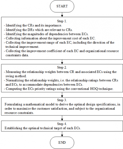
The new HOQ technique is presented in Figure 1.
Figure 1. The proposed HOQ technique
The proposed technique begins by identifying the CRs as the main input for HOQ (step 1). There are three methods which are commonly used for gathering the CRs: interviews, focus groups and observing the product in use [28]. For most products, fifty interviews are possibly too many, but ten interviews are possibly not enough to reveal most of the CRs. As a practical guideline, for a product, thirty interviews might reveal 90 per cent of CRs, whereas 2 hours focus group uncover nearly the same number of CRs as two 1-hour interviews [29].
Then a survey is conducted to assess the importance rating of each CR. For $C R_i$, i=1 to m, the weighted average of importance ratings is computed using Eq. (2).
$d_i^{\text {average }}=\frac{\sum_{n=1}^p Q^{\prime} \cdot n^{\prime}}{Q}$ (2)
where,
$d_i^{\text {average }}$=the importance rating’s weighted average for $C R_i$
$Q^{\prime}=$ number of respondents at rating $n^{\prime}$ (a $p^{\prime}$ point scale rating is used)
Q= total number of respondents
For the purpose of optimization model, $d_i^{\text {average }}$ is normalized, so that the sum of $d_i^{\text {average }}$ for all $C R_i$ is equal to one (see Eq. (3)).
$d_i^{\text {average }}=\frac{\sum_{n=1}^p Q^{\prime} \cdot n^{\prime}}{Q}$ (3)
$D_i=$ the normalized importance of the $C R_i$
After the CRs are identified, the associated $E C_j, j=1$ to $n$, are generated, as technical metrics of CRs, and the magnitudes of dependencies between ECs are assessed. All of the correlation values between $E C_j$ and $E C_k$, denoted as $\gamma_{j k}$, are placed on the top (the roof part) of HOQ.
Next, the technically achievable range for each EC is described, including its direction of improvement. The technically achievable range restricts the improvement span for EC, thus, the technically achievable range can be considered as the improvement range. For $E C_j$, the improvement range is defined by the lower bound $L_j$ and upper bound $U_j$. In designing commercial products, the marginally acceptable range may be used as an additional constraint to the improvement span. Marginally acceptable range of certain EC represents the technical range that would just barely make the product commercially viable [28].
Also, information regarding the resource constraints is collected. The organizational resource constraint maybe described as the amount available cost and/or time to make improvement. The improvement coefficients $\left(C_j\right)$, which represent the amount of resource needed to make a unit improvement of $E C_j$, need to be identified in defining a resource constraint. In this paper, the amount of available organizational resource is denoted by B.
In step 2, the swing method is applied to assess the relationship weight between CRs and ECs. Swing method is commonly used to assess the weights in an additive multi attribute utility function. Next, the normalization procedure (see Eq. (1)) is applied to the relationship ratings, to accommodate the dependencies between ECs. The priority ratings of each EC are computed using the conventional HOQ technique as shown by Eq. (4).
$A_j=\sum_{i=1}^m D_i \cdot R_{i, i}^{\text {norm }} \forall_j$ (4)
where,
$A_j$= the absolute priority rating of the $E C_j$
Afterward, an optimization model is constructed (step 3). The complete formulation is presented by Eq. (5) to Eq. (7).
$\operatorname{Max} Z=\sum_{j=1}^n A_j \cdot X_j$ (5)
Subject to $\forall_j ; X_j=\left\lceil\frac{T_j-U_j}{U_j-L_j}\right\rceil$ for the case the smaller the better, or
$X_j=\frac{T_j-U_j}{U_j-L_j}$ for the case the larger the better (6)
$\sum_{i=1}^n C_j \cdot X_j \leq B$ (7)
where,
$Z=$ the achieved customer satisfaction level
$L_j=$ the lower limit of the improvement range of $E C_j$
$U_j=$ the upper limit of the improvement range of $E C_j$
$T_j=$ the technical target of $E C_j$
$X_j=$ the percentage of the technical improvement of $E C_j$
$C_j=$ the improvement coefficient of $E C_j$
$B=$ the amount of available resource for design improvement
The optimal design specifications are obtained by solving the optimization model to find the optimal technical target ($T_j$) for all j (step 4).
The illustrative the new HOQ technique, an example of designing a wooden dining chair is presented. The first step in implementation of the new HOQ procedure is collecting input data. A survey conducted to identify the CRs of a dining chair. Thirty lead users were intensively interviewed. The interview results revealed that there are five CRs. Then, the second survey was conducted. 263 respondents filled the questionnaires to assess the importance of CRs in a four-point scale. For $C R_i$, the weighted average of the importance ratings ( $d_i^{\text {average }}$) was computed using Eq. (2). As an example, $d_i^{\text {average }}$ was computed as follows. The respondents' assessment results for $C R_i$ showed that there were 4 respondents assigned the value of 1, 20 respondents assigned the value of 2, 80 respondents assigned the value of 3 and 159 assigned the value of 4. Then, $d_i^{average}=\frac{(4 \times 1)+(20 \times 2)+(80 \times 3)+(159 \times 4)}{263}$, so $d_i^{\text {average }}$ is equal to 3.498.
Next, $d_i^{average}$ were normalized using Eq. (3) to obtain $D_i$, for all $i$. Description of $C R_i$ and the associated $d_i^{average}$ for all $i$ are shown by Table 1.
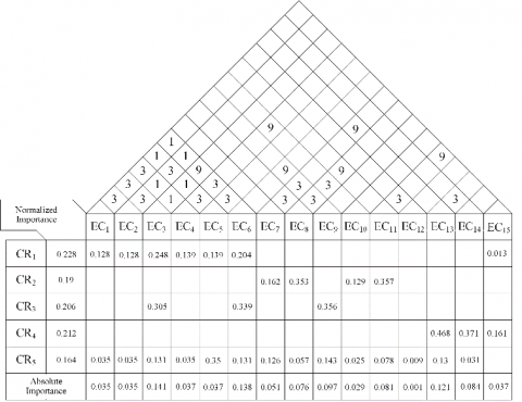
The weight of customer needs is obtained by dividing the average weight of each customer requirement by their total sum so that weight for CR1, CR2, CR3, CR4 and CR5 are 0.228, 0.188, 0.206, 0.212. 0.164 respectively. Fifteen related ECs were generated to represent the CRs identified. Then, all $\gamma_{j k}$, improvement spans (denoted by $L_j$ and $U_j$) and the direction of improvements were defined (as presented by Table 2). The improvement ranges were established with respect to technically achievable ranges and human anthropometry.
Meanwhile, the design team also collected the data concerning the resource constraint (i.e., $C_j$ for all $j$ and $B$). The existing dining chair was designed in the worst specifications, so it produced the worst customer satisfaction level (0%). There were some available resources to improve the dining chair design. In this case example, B was represented by the cost budget and $C_j$ represented the cost needed to make a percentage improvement of $E C_j$.
Table 1. Customer requirement list
|
|
Description |
$d_i^{average}$ |
|
$C R_1$ |
Robust |
3.498 |
|
$C R_2$ |
Unhampered seat |
2.890 |
|
$C R_3$ |
Right height from the ground |
3.171 |
|
$C R_4$ |
Comfortable back of seat |
3.262 |
|
$C R_5$ |
Light weighted |
2.521 |
Table 2. Engineering characteristics list
|
|
Description |
Improvement Range |
Description of Improvement |
|
$EC_1$ |
Length of front leg |
5-7 cm |
The larger the better |
|
$EC_2$ |
Width of front leg |
5-7 cm |
The larger the better |
|
$EC_3$ |
Height of front leg |
39.5-41.5 cm |
The smaller the better |
|
$EC_4$ |
Length of back leg |
5-7 cm |
The larger the better |
|
$EC_5$ |
Width of back leg |
5-7 cm |
The larger the better |
|
$EC_6$ |
Height of back leg |
39.5-41.5 cm |
The smaller the better |
|
$EC_7$ |
Width of seat |
53.6-58.6 cm |
The larger the better |
|
$EC_8$ |
Length of seat |
42.4-45 cm |
The larger the better |
|
$EC_9$ |
Seat thickness |
1.2-4 cm |
The larger the better |
|
$EC_{10}$ |
Height of arm rest |
23-24.5 cm |
The smaller the better |
|
$EC_{11}$ |
Length of arm rest |
30.7-33.7 cm |
The smaller the better |
|
$EC_{12}$ |
Width of arm rest |
9.1-10.8 cm |
The larger the better |
|
$EC_{13}$ |
Width of back of seat |
43-46.6 cm |
The larger the better |
|
$EC_{14}$ |
Length of back of seat |
55.3-59.9 cm |
The larger the better |
|
$EC_{15}$ |
Angle of back of seat (and horizontal axis) |
90-100° |
The larger the better |
The available cost budget was IDR 10000. Cj for j=1 to 15 were as follows: 2312.02, 2312.02, -881.7, 2312.02, 2312.02, -881.7, 20047.35, 15858.35, 8067.864, -395.595, -711.24, 1222.436, 3837.169, 3974.722, 0. In this case, Cj mostly concerned with the material cost and the negative values of Cj were defined for ECj with the smaller the better characteristic.
Then, the second step of the proposed technique was conducted. A technical expert was asked to assess the relationship weight between CRs and ECs using the swing method as follows:
(1) Two alternative designs were shown to the technical team, one leads to the worst specifications and the other leads to the best.
(2) The team was asked to rank the ECs, one by one, by specifying which EC that has the most significant impact on satisfying a certain CR if its value swings from the worst to the best.
(3) EC with the most significant impact on satisfying CR would obtain the value of 100. The other EC would be compared to the most significant and would be rated proportionally on 0-100 scale. The completely irrelevant EC would gain the weight of 0. The results are shown on Table 3.
The normalization procedure was employed so that the sum of the weights is equal to one, as can be seen in Table 4.
Table 3. The impact ratings of ECs to CRs
|
|
EC1 |
EC2 |
EC3 |
EC4 |
EC5 |
EC6 |
EC7 |
EC8 |
EC9 |
EC10 |
EC11 |
EC12 |
EC13 |
EC14 |
EC15 |
|
CR1 |
50 |
50 |
70 |
50 |
50 |
100 |
|
|
|
|
|
|
|
|
70 |
|
CR2 |
|
|
|
|
|
|
100 |
80 |
|
30 |
30 |
|
|
|
|
|
CR3 |
|
|
100 |
|
|
80 |
|
|
70 |
|
|
|
|
|
|
|
CR4 |
|
|
|
|
|
|
|
|
|
|
|
|
50 |
80 |
100 |
|
CR5 |
20 |
20 |
40 |
20 |
20 |
40 |
100 |
70 |
70 |
20 |
20 |
20 |
70 |
70 |
|
Table 4. The normalized impact ratings of ECs to CRs
|
|
EC1 |
EC2 |
EC3 |
EC4 |
EC5 |
EC6 |
EC7 |
EC8 |
EC9 |
EC10 |
EC11 |
EC12 |
EC13 |
EC14 |
EC15 |
|
CR1 |
0.114 |
0.114 |
0.159 |
0.114 |
0.114 |
0.227 |
|
|
|
|
|
|
|
|
0.159 |
|
CR2 |
|
|
|
|
|
|
0.417 |
0.333 |
|
0.125 |
0.125 |
|
|
|
|
|
CR3 |
|
|
0.400 |
|
|
0.32 |
|
|
0.280 |
|
|
|
|
|
|
|
CR4 |
|
|
|
|
|
|
|
|
|
|
|
|
0.217 |
0.348 |
0.435 |
|
CR5 |
0.033 |
0.033 |
0.067 |
0.033 |
0.067 |
0.067 |
0.167 |
0.117 |
0.117 |
0.033 |
0.033 |
0.033 |
0.117 |
0.117 |
|
Then, the other normalization procedure (Eq. (1)) was employed to the normalized weights. The normalization results were arranged in the relationship matrix of the HOQ. The example of normalization for R33 is as follows:
$R_{33}^{\text {norm }}=\frac{R_{33} \cdot \gamma_{33}+R_{36} \cdot \gamma_{63}+R_{39} \cdot \gamma_{93}}{R_{33} \cdot \gamma_{33}+R_{36} \cdot \gamma_{63}+R_{39} \cdot \gamma_{93}+R_{33} \cdot \gamma_{63}+R_{36} \cdot \gamma_{66}+R_{39} \cdot \gamma_{96}+R_{33} \cdot \gamma_{93}+R_{36} \cdot \gamma_{69}+R_{39} \cdot \gamma_{99}}$
$R_{33}^{\text {norm }}=\frac{(0.4 * 1)+(0.32 * 9)+(0.28 * 9)}{(0.4 * 1)+(0.32 * 9)+(0.28 * 9)+(0.4 * 9)+(0.32 * 1)+(0.28 * 9)+(0.4 * 9)+(0.32 * 9)+(0.28 * 1)}$
Later, the absolute importance for the $E C_j$ (that is $A_j$) were computed for all $j$ (Eq. (4)). For example: $A_1=(0.228 *$ $0.128)+(0.164 * 0.035)=0.035$.
Then, the complete HOQ matrix could be developed as shown by Figure 2.
Figure 2. The complete HOQ for a dining chair design
Table 5. Optimal solution
|
Variable |
Value |
Variable |
Value |
|
$T_1$ |
5 cm |
$X_1$ |
0% |
|
$T_2$ |
5.376 cm |
$X_2$ |
18.784% |
|
$T_3$ |
39.5 cm |
$X_3$ |
100% |
|
$T_4$ |
7 cm |
$X_4$ |
100% |
|
$T_5$ |
7 cm |
$X_5$ |
100% |
|
$T_6$ |
39.5 cm |
$X_6$ |
100% |
|
$T_7$ |
53.6 cm |
$X_7$ |
0% |
|
$T_8$ |
42.4 cm |
$X_8$ |
0% |
|
$T_9$ |
1.2 cm |
$X_9$ |
0% |
|
$T_{10}$ |
23 cm |
$X_{10}$ |
100% |
|
$T_{11}$ |
30.7 cm |
$X_{11}$ |
100% |
|
$T_{12}$ |
9.1 cm |
$X_{12}$ |
0% |
|
$T_{13}$ |
46.6 cm |
$X_{13}$ |
100% |
|
$T_{14}$ |
59.9 cm |
$X_{14}$ |
100% |
|
$T_{15}$ |
100° |
$X_{15}$ |
100% |
The third step is formulating the optimization model. The appropriate mathematical model is presented by Eq. (8) to Eq. (24).
$\begin{aligned} & \operatorname{Max} Z=0.035 \mathrm{X}_1+0.035 \mathrm{X}_2+0.141 \mathrm{X}_3+0.037 \mathrm{X}_4 \\ & \quad+0.037 \mathrm{X}_5+0.138 \mathrm{X}_6+0.051 \mathrm{X}_7+0.076 \mathrm{X}_8 \\ & \quad+0.097 \mathrm{X}_9+0.029 \mathrm{X}_{10}+0.081 \mathrm{X}_{11}+0.001 \mathrm{X}_{12} \\ & \quad+0.121 \mathrm{X}_{13}+0.121 \mathrm{X}_{14}+0.037 \mathrm{X}_{15}\end{aligned}$ (8)
Subject to
$\mathrm{X}_1=\left(\mathrm{T}_1-5\right) /(7-5)$ (9)
$\mathrm{X}_2=\left(\mathrm{T}_2-5\right) /(7-5)$ (10)
$\mathrm{X}_3=\left|\left(\mathrm{T}_3-41.5\right) /(41.5-39.5)\right|$ (11)
$\mathrm{X}_4=\left(\mathrm{T}_4-5\right) /(7-5)$ (12)
$\mathrm{X}_5=\left(\mathrm{T}_5-5\right) /(7-5)$ (13)
$X_6=\left|\left(T_6-41.5\right) /(41.5-39.5)\right|$ (14)
$\mathrm{X}_7=\left(\mathrm{T}_7-53.6\right) /(58.6-53.6)$ (15)
$\mathrm{X}_8=\left(\mathrm{T}_8-42.4\right) /(45-42.4)$ (16)
$X_9=\left(T_9-1.2\right) /(4-1.2)$ (17)
$\mathrm{X}_{10}=\left|\left(\mathrm{T}_{10}-24.5\right) /(24.5-23)\right|$ (18)
$\mathrm{X}_{11}=\left|\left(\mathrm{T}_{11}-33.7\right) /(33.7-30.7)\right|$ (19)
$\mathrm{X}_{12}=\left(\mathrm{T}_{12}-9.1\right) /(10.8-9.1)$ (20)
$\mathrm{X}_{13}=\left(\mathrm{T}_{13}-43\right) /(46.6-43)$ (21)
$\mathrm{X}_{14}=\left(\mathrm{T}_{14}-55.3\right) /(59.9-55.3)$ (22)
$\mathrm{X}_{15}=\left(\mathrm{T}_{15}-90\right) /(100-90)$ (23)
$\begin{gathered}2312.02 \mathrm{X}_1+2312.02 \mathrm{X}_2+\left(-881.7 \mathrm{X}_3\right)+2312.02 \mathrm{X}_4 \\ +2312.02 \mathrm{X}_5+\left(-881.7 \mathrm{X}_6\right)+20047.35 \mathrm{X}_7+15858.35 \mathrm{X}_8 \\ +8067.864 \mathrm{X}_9+\left(-395.595 \mathrm{X}_{10}\right)+\left(-711.24 \mathrm{X}_{11}\right) \\ +1222.436 \mathrm{X}_{12}+3837.169 \mathrm{X}_{13}+3974.722 \mathrm{X}_{14} \\ +(0) \mathrm{X}_{15} \leq 10000\end{gathered}$ (24)
Lingo 19.0 was used to solve the optimization model to derive the optimal specifications. $T_j$ and the associated $X_j$, for all j, are shown in Table 5.
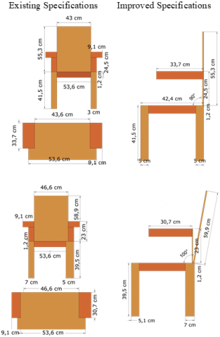
The optimal specifications lead to the customer satisfaction score of 71.15%. The graphical representation of the dining chair with optimal specifications is shown by Figure 3.
Figure 3. Existing and improved design
In the formation of HOQ matrix, several pieces of information are required, namely customer needs, customer importance weights, technical characteristics, CRs and ECs relationships, ECs relationships and absolute importance. The relationship ratings between ECs have been normalized. With this normalization, it is expected that new priorities can be formed as it accommodates the relationships between engineering characteristics. For example, comfortable back of seat (CR4), which is related to engineering characteristic backrest position (EC15), before normalization, EC15 was the dominant characteristic influencing CR4 with a rating value of 0.435. However, after normalization, EC15 becomes non-dominant, with a value of 0.16. This is because EC15 does not have a relationship with other engineering characteristics (in this case, EC13 and EC14).
To determine customer satisfaction level, it has been expressed with mathematical Eq. (5). Xj represents the percentage of technical improvement of $E C_j$ with values ranging from 0 to 1, and Aijis the absolute priority rating of the $EC_j$. The maximum value obtained for customer satisfaction is 1 (100%). The range constraint of $E C_j$ is established with Eq. (6), where Ti represents the technical target of $E C_j$ with lower and upper limit of the improvement range $EC_j$ Another main constraint is the product development cost represented by Eq. (7). If there is no improvement in $EC_j$, then the value of Ci for that $EC_j$ will be 0.
We can see from Table 5 the optimal solution, it is apparent that for X1, X7, X8, X9, and X12, the values are 0, indicating that their performance is within the minimum range of characteristics or equal to the initial characteristics. Conversely, X3, X4, X5, X6, X10, X11, X13, X14, and X15 are within the performance range of maximum characteristics.
The sensitivity analysis was conducted to determine the change in budget towards customer satisfaction. Table 6 illustrates the contribution of budget changes for every increase of 1000 IDR towards the improvement of customer satisfaction. In this numerical example, the given budget is 10000 IDR, resulting in a customer satisfaction level of 71.15% at this budget.
Table 6. Sensitivity analysis on budget change to customer satisfaction improvement
|
Budget (IDR) |
Customer Satisfaction (%) |
Delta |
|
1000 |
54.77 |
|
|
2000 |
56.88 |
2.11 |
|
3000 |
58.99 |
2.11 |
|
4000 |
61.11 |
2.12 |
|
5000 |
63.19 |
2.08 |
|
6000 |
64.79 |
1.60 |
|
7000 |
66.39 |
1.60 |
|
8000 |
67.99 |
1.60 |
|
9000 |
69.59 |
1.60 |
|
10000 |
71.15 |
1.56 |
|
11000 |
72.67 |
1.52 |
|
12000 |
74.19 |
1.52 |
|
13000 |
75.70 |
1.51 |
|
14000 |
77.20 |
1.50 |
|
15000 |
78.47 |
1.27 |
|
16000 |
79.67 |
1.20 |
|
17000 |
80.88 |
1.21 |
|
18000 |
82.08 |
1.20 |
|
19000 |
83.28 |
1.20 |
|
20000 |
84.48 |
1.20 |
|
21000 |
85.68 |
1.20 |
|
22000 |
86.89 |
1.21 |
|
23000 |
87.55 |
0.66 |
|
24000 |
88.03 |
0.48 |
|
25000 |
88.51 |
0.48 |
|
26000 |
88.99 |
0.48 |
|
27000 |
89.47 |
0.48 |
|
28000 |
89.95 |
0.48 |
|
29000 |
90.43 |
0.48 |
|
30000 |
90.91 |
0.48 |
Table 6 indicates that an increase in the budget by 1000 IDR results in a customer satisfaction improvement of approximately 2%. However, when the budget exceeds 23000 IDR, the increase in customer satisfaction becomes insignificant, reaching only 0.48%.
This paper has proposed a formal HOQ technique to determine the technical target of ECs. The swing method and Wasserman’s normalization procedure was employed to obtain better relationship ratings. A mathematical model was developed to maximize customer satisfaction, subject to available organizational resources. The proposed procedure was applied in designing a wooden dining chair and has improved the customer satisfaction. A sensitivity analysis has been conducted to obtain the optimal budget to yield customer satisfaction.
Several contributions to the body of knowledge have been obtained to offer a new mathematical model. First, this study contributes to the using of weighted average of the importance rating to convert the customer requirements to engineering characteristics. Second, this study contributes to the engineering characteristics relationship ratio to incorporating the effect of dependencies. Also, contributions to product development practitioners by providing mathematical models and their procedures facilitate practitioners in translating consumer desires into technical characteristics to achieve optimal consumer satisfaction within technical specifications and cost constraints, with detailed numerical example.
However, the proposed technique still used ratings which were measured on interval (even on ordinal scale) i.e. CRs’ importance ratings and correlation between ECs. For future research, better weighting methods need to be employed to assess those values.
[1] Seker, S., Aydin, N. (2023). Fermatean fuzzy based quality function deployment methodology for designing sustainable mobility hub center. Applied Soft Computing, 134: 110001. https://doi.org/10.1016/j.asoc.2023.110001
[2] Lai, X., Xie, M., Tan, K.C. (2006). QFD optimization using linear physical programming. Engineering Optimization, 38(5), 593-607. https://doi.org/10.1080/03052150500448059
[3] Zhou, J., Shen, Y., Pantelous, A.A., Liu, Y. (2022). Quality function deployment: A bibliometric-based overview. IEEE Transactions on Engineering Management, 71: 1180-1201. https://doi.org/10.1109/TEM.2022.3146534
[4] Akao, Y. (1990). History of quality function deployment in Japan. The Best on Quality: Targets, Improvement, Systems, 3: 183-196.
[5] Akao, Y., Mazur, G.H. (2003). The leading edge in QFD: Past, present and future. International Journal of Quality & Reliability Management, 20(1): 20-35. https://doi.org/10.1108/02656710310453791
[6] Lombardi, M., Garzia, F., Fargnoli, M., Pellizzi, A., Ramalingam, S. (2020). Application of quality function deployment to the management of information physical security. International Journal of Safety and Security Engineering, 10(6): 727-732. https://doi.org/10.18280/ijsse.100601
[7] Agarwal, A., Ojha, R. (2023). Prioritising the determinants of Industry-4.0 for implementation in MSME in the post-pandemic period–a quality function deployment analysis. The TQM Journal, 35(8): 2181-2202. https://doi.org/10.1108/TQM-06-2022-0204
[8] Abdul Rahman, K., Ahmad, S.A., Che Soh, A., Ashari, A., Wada, C., Gopalai, A.A. (2023). Improving fall detection devices for older adults using quality function deployment (QFD) approach. Gerontology and Geriatric Medicine, 9: 23337214221148245. https://doi.org/10.1177/23337214221148245
[9] Yulius, H., Dewata, I., Heldi, Putra, A. (2023). Designing eco-friendly Kambuik shopping bags: A quality function deployment approach. International Journal of Design & Nature and Ecodynamics, 18(6): 1469-1474. https://doi.org/10.18280/ijdne.180621
[10] Khandoker, A., Sint, S., Gessl, G., et al. (2022). Towards a logical framework for ideal MBSE tool selection based on discipline specific requirements. Journal of Systems and Software, 189: 111306. https://doi.org/10.1016/j.jss.2022.111306
[11] Franceschini, F., Rossetto, S. (1998). Quality function deployment: How to improve its use. Total Quality Management, 9(6): 491-500. https://doi.org/10.1080/0954412988424
[12] Askin, R.G., Dawson, D.W. (2000). Maximizing customer satisfaction by optimal specification of engineering characteristics. IIE Transactions, 32(1): 9-20. https://doi.org/10.1080/07408170008963875
[13] Park, T., Kim, K.J. (1998). Determination of an optimal set of design requirements using house of quality. Journal of Operations Management, 16(5): 569-581. https://doi.org/10.1016/S0272-6963(97)00029-6
[14] Wang, Z.Q., Chen, Z.S., Garg, H., Pu, Y., Chin, K.S. (2022). An integrated quality-function-deployment and stochastic-dominance-based decision-making approach for prioritizing product concept alternatives. Complex & Intelligent Systems, 8(3): 2541-2556. https://doi.org/10.1007/s40747-022-00681-1
[15] Shi, H., Mao, L.X., Li, K., Wang, X.H., Liu, H.C. (2022). Engineering characteristics prioritization in quality function deployment using an improved ORESTE method with double hierarchy hesitant linguistic information. Sustainability, 14(15): 9771. https://doi.org/10.3390/su14159771
[16] Xiao, J., Wang, X. (2024). An optimization method for handling incomplete and conflicting opinions in quality function deployment based on consistency and consensus reaching process. Computers & Industrial Engineering, 187: 109779. https://doi.org/10.1016/j.cie.2023.109779
[17] Ping, Y.J., Liu, R., Lin, W., Liu, H.C. (2020). A new integrated approach for engineering characteristic prioritization in quality function deployment. Advanced Engineering Informatics, 45: 101099. https://doi.org/10.1016/j.aei.2020.101099
[18] Mistarihi, M.Z., Okour, R.A., Mumani, A.A. (2020). An integration of a QFD model with Fuzzy-ANP approach for determining the importance weights for engineering characteristics of the proposed wheelchair design. Applied Soft Computing, 90: 106136. https://doi.org/10.1016/j.asoc.2020.106136
[19] Kang, X., Nagasawa, S.Y. (2023). Integrating continuous fuzzy Kano model and fuzzy quality function deployment to the sustainable design of hybrid electric vehicle. Journal of Advanced Mechanical Design, Systems, and Manufacturing, 17(2): JAMDSM0019-JAMDSM0019. https://doi.org/10.1299/jamdsm.2023jamdsm0019
[20] Lim, C.H., Chin, J.F. (2023). V-model with fuzzy quality function deployments for mobile application development. Journal of Software: Evolution and Process, 35(1): e2518. https://doi.org/10.1002/smr.2518
[21] Aydin, N., Seker, S., Deveci, M., Ding, W., Delen, D. (2023). A linear programming-based QFD methodology under fuzzy environment to develop sustainable policies in apparel retailing industry. Journal of Cleaner Production, 387: 135887. https://doi.org/10.1016/j.jclepro.2023.135887
[22] Xing, Y., Liu, Y., Davies, P. (2023). Servitization innovation: A systematic review, integrative framework, and future research directions. Technovation, 122: 102641. https://doi.org/10.1016/j.technovation.2022.102641
[23] Liu, Q., Chen, X., Tang, X. (2024). Spherical fuzzy bipartite graph based QFD methodology (SFBG-QFD): Assistive products design application. Expert Systems with Applications, 239: 122279. https://doi.org/10.1016/j.eswa.2023.122279
[24] Erdil, N.O., Arani, O.M. (2018). Quality function deployment: More than a design tool. International Journal of Quality and Service Sciences, 11(2): 142-166. https://doi.org/10.1108/IJQSS-02-2018-0008
[25] Dewi, D.R.S., Rahaju, D.E.S. (2016). An integrated QFD and kano's model to determine the optimal target specification. In 2016 International Conference on Industrial Engineering, Management Science and Application (ICIMSA), Jeju, Korea (South), pp. 1-5. https://doi.org/10.1109/ICIMSA.2016.7503991
[26] Dewi, D.R.S., Debora, J., Sianto, M.E. (2017). Dealing with dissatisfaction in mathematical modelling to integrate QFD and Kano’s model. IOP Conference Series: Materials Science and Engineering, 277(1): 012009. https://doi.org/10.1088/1757-899X/277/1/012009
[27] Dewi, D.R.S., Hermanto, Y.B. (2022). Supply chain capabilities to improve sustainability performance of product-service systems. International Journal of Sustainable Development and Planning, 17(8): 2561-2569. https://doi.org/10.18280/ijsdp.170824
[28] Ulrich, K.T., Eppinger, S.D. (2016). Product Design and Development. McGraw-hill.
[29] Griffin, A., Hauser, J.R. (1993). The voice of the customer. Marketing Science, 12(1): 1-27. https://doi.org/10.1287/mksc.12.1.1