Saci Taraft![]() | Djamila Rekioua*
| Djamila Rekioua*![]() | Abdelhak Djoudi
| Abdelhak Djoudi![]() | Seddik Bacha
| Seddik Bacha![]() | Djamel Aouzellag
| Djamel Aouzellag![]()
© 2024 The authors. This article is published by IIETA and is licensed under the CC BY 4.0 license (http://creativecommons.org/licenses/by/4.0/).
OPEN ACCESS
In this paper, the operation of an inertial flywheel storage system based on the permanent magnet synchronous machine (PMSM) is presented. The contribution in this work lies in the optimization of the exchanged power between the storage system and the grid. The related speed reference is determinate from the desired power through a tracking algorithm known as reference power point tracking (RPPT). This one permit to achieve a desired grid-side power. That is ensured by a simple algorithm which needs only the measurements of grid-side power and reference power. This algorithm is robust because it doesn’t depend to system parameters, and to an increased reliability. The problem of variable losses once several grid connected-storage systems are considered is then avoided. This will serve grid operator to adjust efficiently the grid frequency. The last point is the main advantage of the proposed method compared with others ones that use machine-side power measurements for speed reference synthetizing. The studied system is implemented under DSPACE type RTI1005. The rotation speed of the permanent magnet machine and the power exchanged between the electrical grid and the inertial storage system follow their reference with an error of 0.032% and 0.83% respectively. The simulation and experimental results presented show the effectiveness of the tracking algorithm.
static converter, inertial storage, permanent magnet synchronous machine, reference power point tracking algorithm
More and more the world is converging to the exploitation of electrical energy; As a result, electricity consumption continues to increase in considerable quantities. Nowadays, most of electrical networks are powered from power stations that use fossil-type primary energy. This energy on the one hand is limited in stocks, on the other pollutes the atmosphere, negative alteration of the climate namely the release of greenhouse gases. This will result in a consequent rise in temperature of the planet earth. This fact affects human health and ecological balance. The ideal would be to minimize the use of fossil energy, contribute to the purification of the environment and meet the high demand for electricity. This involves the integration of renewable resources, including unlimited human-scale stocks, into the electricity grid.
Various contributions and studies related to wind energy systems, with a focus on control techniques, fault management, optimization, and energy storage are presented in this work. The studies in references [1-4] mention various applications and methodologies related to wind energy systems. In the study of Hassani et al. [1] presented the application of a control technique to double the nominal power generated by the wind turbine. The capacity and fault management in an integrated micro-wind conversion system are improved via adaptive control [2]. The optimization criterion in order to minimize the cost of energy while taking into account the level of reliability required by the consumer is proposed by Djamila et al. [3]. Similarly, Mebarki et al. [4] proposed a systematic methodology to optimize the costs of an offshore wind farm based on a supervisory level frame work. These contributions present an attractive and alternative solution to fossil resources. However, their development is slowed down and considered as negative charges and does not contribute to system services or the protection of the electrical grid. This is first due to their primary sources which stochastic nature; therefore, do not participate in system services.
Otherwise, their rates of integration into the grid are limited to 30% of the capacity of the grid [5]. From these considerations it emerges that the stability of the network does not only depends on the reinforcement in electrical energy but on the quality of the power injected into the grid. This state should change and consciously thought to integrate the means of storage in the intermittent resources, which can make it acquire the smoothing property of the power injected into the network, and therefore, crossing the penetration barrier to the network and participate in the system service. Indeed, the integration of the storage system contributes to the valorization of intermittent and renewable energy production systems [6].
Many works are developed on energy storage systems; among these, there is the electromechanical storage, generally integrated in generators whose primary energy is stochastic. The aim of integrating this type of storage into generating systems is, in one hand, to increase the penetration rate of the generators to the micro-networks [7, 8] and, in the other hand, to participate in the system service and to improve the quality of the injected power in the grid [9-11]. Therefore, valorize intermittent resources and protect the network against overloads. Ayodele and Ogunjuyigbe [8] have shown the importance of integrating energy storage systems, particularly flywheels, into intermittent energy production units, with a view to reducing intermittency and making the most of renewable resources. But there is no mention of power losses in converters when power is exchanged between the grid and the storage system.
In order to improve the performance of these storage systems, several strategies and control techniques have been applied. Authors have tried to improve the performance of inertial storage systems, taking several steps. All the studies in references [12-15] mention challenges such as errors in current measurement, instability risks, and difficulties in identifying controller parameters. This highlights the need for robust control strategies and accurate parameter identification methods. For example, a control strategy of the synchronous machine driving a flywheel is presented, in order to improve the performance of the inertial storage system, nevertheless, the error during the current measurement increases after the integral, in addition, the speed estimation method using the waveforms is no longer credible [12]. A control technique is used to emulate a flywheel, which is made from the DC machine [13]. A flywheel is driven by the permanent magnet machine, which is controlled by means of a direct frequency matrix-converter [14]. However, for short operating periods there is an instability risk due to errors in the measurement of the stator currents. A new algorithm is proposed be Gamboa et al. [15] to control high-speed flywheels controlled by PID controllers, but, the application of this algorithm, presents difficulties to identify the parameters of the inverter with this controller, which makes sensitive the system control.
Talebi et al. [16] proposed the study of a variable speed wind induction generator associated to a flywheel energy storage system using direct torque control strategy through only simulations. Similarly, low speed PMSG based flywheel energy storage system is integrated with Direct-Drive (DD) variable speed PMSG based wind energy conversion system [17]. Or a flywheel driven by the squirrel-cage induction machine, for which a direct torque control (DTC) and vector modulation are applied to improve the performance of the system [18].
The possibility and interest of grouping inertia flywheels in parallel, and driving them by permanent magnet synchronous motors, has been treated by Xu et al. [19]. Aissou et al. [20] has been shown the interest of replacing mechanical bearings by magnetic ones, which lies in losses reduction. It is noticed there is a lack of mention of power losses in converters during power exchange between the grid and storage systems in some previous studies [21-23]. Considering converter losses is crucial for accurate assessments and system optimization.
In order to value inertial storage, an overview of flywheel technology and previous projects is presented in indeed [21], the work is dedicated to minimizing losses in flywheel design, without taking into account losses in the static converters involved in power exchange between the flywheel and the electrical grid. Bolund et al. [22] have demonstrated the possibility to compensate the reactive power, by integrating an inertial storage system in the wind turbine conversion system. It can be also found by Aissou et al. [23] that the role played by the inertial storage system associated with wind generators connected to the grid in. In the works above-cited, the reference of the power to be stored and restored is determined from the electromagnetic power. This method does not take into account the power lost in the static and dynamic converters. Therefore, the real power involved between the grid and the storage system is not reached, the correction of the latter is essential in order to stabilize the electrical grid [24].
To overcome this constraint, a new tracking algorithm for the storage power is proposed in this paper. The inertial storage system is made up with a flywheel and permanent magnet synchronous machine injecting power into the grid through power electronic interface. The proposed model will be implemented and simulated in Matlab/Simulink environment. The obtained results are commented and confirmed by comparison with experimental results. The real implementation is made in the laboratory with an emulated flywheel with a DC motor, for which the torque is programmed via a TMS 320F240-type DSP. Permanent magnet machine is connected to the grid through two back-to-back converters. The VSI are controlled by means of RTI1005-type DSPACE. Three experimental tests are made as follows:
-A test with a desired power profile to validate the operation of the system studied in motor /generator modes;
-A test in motor mode, in which the measured power is the one from the grid side;
-A test in motor mode, in which the measured power is the one from the machine side.
The results will be discussed and compared in order to show the effectiveness of the RPPT algorithm and the importance of operating with grid side power.
2.1 System description
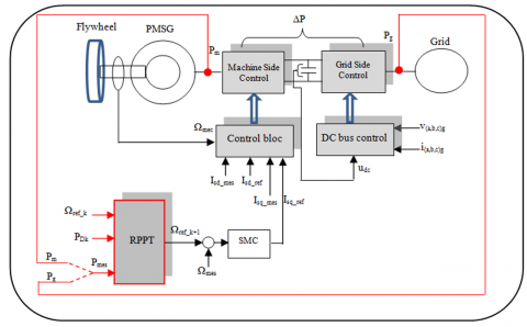
The system proposed in Figure 1 composed of a flywheel and a synchronous machine permanent magnet debited on the network via a static converter (rectifier, filter, and inverter). The set is governed by a flow-oriented pulse width modulated vector control. The power exchanged between the proposed system and the electrical grid depends on the wheel rotation speed, which is determined by the optimization algorithm.
Figure 1. System description
2.2 Flywheel modeling
A flywheel is a moving mass which is circular or non-rotating at Ωv about an axis passing through its gravity center having a kinetic energy quantity Ec. This latter is given by the following expression:
$E_c=\frac{1}{2} J_v \Omega_v^2$ (1)
where, Jv is flywheel inertia.
The calculation of Jv is based on the power to be supplied during a time Δt. It is desired that the inertial storage provides the nominal power Pn during this time (Δt).
The necessary energy is then:
$\Delta E_c=P_n \Delta t$ (2)
With,
$\begin{gathered}\Delta E_c=\frac{1}{2} J_v \Delta \Omega_v^2 \text { and } \Delta \Omega_v^2=\Omega_{v \max }^2-\Omega_{v \min }^2 \\ J_v=\frac{2 P_n \Delta t}{\left(\Omega_{v \max }^2-\Omega_{v \min }^2\right)}\end{gathered}$ (3)
The maximum rotation speed of the flywheel depends on the characteristics of the flywheel material.
$\Omega_{v \max }=s \frac{1}{r} \sqrt{\frac{\sigma}{\rho}}$ (4)
where, s is operational safety factor of the flywheel; σ is tensile strength, ρ is density of the material (kg/m3); r is radius of the flywheel.
The wheel rotation speed during the discharge period is expressed as follows [15]:
$\Omega(t)= \begin{cases}\Omega_{v \max }, & t<\Delta t \\ \Omega_{v \max } . e^{-\frac{k_0}{J_v} t}, & t \geq \Delta t\end{cases}$ (5)
This will result in the expression of the restored power as follows:
$P= \begin{cases}P_n, & t<\Delta t \\ P_n \cdot e^{-\frac{k_0}{J_v} t}, & t \geq \Delta t\end{cases}$ (6)
From these equations, we find that the choice of the flywheel depends on two initial conditions, which must be taken into account; namely the maximum rotation speed of the flywheel and its capacity.
2.3 Permanent magnet synchronous generator modeling
The synchronous machine is chosen according to its advantages in terms of simplicity, absence of brushes, increase in speed, reduction of losses compared to the asynchronous machine, in addition, it has interesting mass volume and of easy control (the flux not estimated).
2.3.1 Electric equations
The voltages equations of the machine in the Park frames are given by Eq. (7) and Eq. (8) [25]:
$\left\{\begin{array}{l}v_q=\left(R_s+S L_q\right) i_q+\omega_e L_d i_d+\omega_e \psi_r \\ v_d=\left(R_s+S L_d\right) i_d-\omega_e L_q i_q\end{array}\right.$ (7)
$\left\{\begin{array}{l}\frac{d i_d}{d t}=-\frac{R_s}{L_d} i_d+\omega_e \frac{L_q}{L_d} i_q+\frac{v_d}{L_d} \\ \frac{d i_q}{d t}=-\frac{R_s}{L_q} i_q-\omega_e \frac{L_d}{L_q} i_d-\frac{1}{L_q} \psi_r \omega_e+\frac{v_q}{L_q}\end{array}\right.$ (8)
The electromagnetic torque Tem of the machine is the result of the interaction between the poles formed by the magnets at the rotor and the poles generated by the magnetomotive forces FMMs in the air gap generated by the stator currents [26-29].
$T_{e m}=\frac{3}{2} P\left[\psi_r i_q-\left(L_d-L_q\right) i_d i_q\right]$ (9)
2.3.2 Mechanical equations [26]
During the operation of the machine, the rotating part is subjected to torques, namely electromagnetic torque, load torque and friction torque, Tem, Tr and Tf respectively (Figure 2).
The dynamic fundamental expression of the system is given as follows:
$J \frac{d \Omega}{d t}=\sum_i T_i$ (10)
$J \frac{d \Omega}{d t}=T_{e m}-T_r-T_f$ (11)
$T_f=f * \Omega$ (12)
where, $J$ is inertia of the motor; $f$ is viscous friction coefficient, $T_f$ is friction torque; $T_{e m}$ is electromagnetic torque delivered by the motor; $T_r$ is resistant torque, or load; $\Omega$ is mechanical rotation speed.
Figure 2. Different torques acting on the rotor of the machine
The bidirectional power converter consists of two conventional pulse width modulated (PWM) voltage source converters (VSC) [26, 27]. The first one is a rectifier while the second is an inverter. These two converters share the same DC-link (Figure 3).
Figure 3. The back-to-back rectifier-inverter converter
3.1 Rectifier modeling
The relation between AC and DC sides of the rectifier is given by the following relation.
$\left[\begin{array}{l}V_{d c}^{+} \\ V_{d c}^{-}\end{array}\right]=\left[\begin{array}{lll}S_1 & S_3 & S_5 \\ S_2 & S_4 & S_6\end{array}\right]\left[\begin{array}{l}v_a \\ v_b \\ v_c\end{array}\right]$ (13)
where, Si is a connection function of associated with each switch in the rectifier (i=1,2,…,6). The DC-link voltage is obtained as:
$V_c=V_{d c}^{+}-V_{d c}^{-}$ (14)
In the same way we can express DC current $i_{\text {rec}}$ according to the AC currents as:
$i_{r e c}=\left[\begin{array}{lll}S_1 & S_3 & S_5\end{array}\right]\left[\begin{array}{l}i_a \\ i_b \\ i_c\end{array}\right]$ (15)
3.2 Filter modeling
The filter used in this paper is a low pass. It is represented in Figure 4.
Figure 4. Presentation of a low-pass filter
The model of the filter is defined by the following system of equation.
$\begin{gathered}i_{\text {rec }}-i_{\text {inv }}=C \frac{d v_c}{d t} \\ V_C(t)=V_C(0)+\frac{1}{C} \int_{t_1}^{t_2}\left(i_{\text {rec }}-i_{\text {inv }}\right) d t\end{gathered}$ (16)
The capacitor C represents the input DC-voltage for the inverter input, in order to supply reactive energy to the machine, and to absorb the negative current restored by the load.
3.3 Inverter modeling
The voltage inverter ensures the conversion of continuous energy to alternative current (DC/AC). Output voltages are governed by Eq. (17).
$\left[\begin{array}{l}v_A \\ v_B \\ v_C\end{array}\right]=\frac{V_c}{3}\left[\begin{array}{ccc}2 & -1 & -1 \\ -1 & 2 & -1 \\ -1 & -1 & 2\end{array}\right]\left[\begin{array}{l}S_7 \\ S_9 \\ S_{11}\end{array}\right]$ (17)
where, Si is a function of connection associated with each switch of the inverter (i=7, 8, …, 12).
The two converters, i.e., rectifier and inverter are PWM controlled. These converters consist of three arms formed with electronic switches chosen essentially according to the power and the commutation frequency. Each arm has two complementary power components provided with freewheel diode. This diode ensures the continuity of the current in the machine once the switch is open.
The vector control of the AC machine is to bring back its behavior to that of the DC machine. To carry out a control similar to that of DC machines with separate excitation, it is necessary to maintain to zero the current Id, and to regulate the speed or the position using the current Iq by means of the voltage Vq [30].
The system of Eq. (7) becomes:
$\left\{\begin{array}{l}v_q=\left(R_s+S L_q\right) i_q+\omega_e \psi_f \\ v_d=-\omega_e L_q i_q\end{array}\right.$ (18)
And the expression of the electromagnetic torque Eq. (9) becomes:
$T_e=\frac{3}{2} P \psi_r i_q$ (19)
This section is dedicated to elaborate a tracking algorithm allowing to find the speed reference $\Omega_{r e f}$ which permits to track a given reference of grid-side power $P_D$ set by power system operator in order to adjust the grid frequency.
The relation between the mechanical power $P_{\text {mec }}$ and gridside one $P_g$ is given by the relation Eq. (20).
$P_{m e c}=P_g+\Delta_P$ (20)
where, $P_{\text {mec }}$ is the algebraic value of the mechanical power. It is considered that $P_m>0$ once the machine is under motor mode and $P_{\text {mec }}<0$ if the machine is under generator mode. The same is applied for the grid-side power. $\Delta_P$ is power losses of the machine and the converters and it is also algebraic. $\Delta_{\mathrm{P}}<$ 0 if the machine is under motor mode, and $\Delta_{\mathrm{P}}>0$ if the machine is under generator mode.
It is given that:
$P_{\text {mec }}=T_r \Omega$ (21)
The last relation implies:
$P_{m e c}=\Omega\left(T_{e m}-T_f-J \frac{d \Omega}{d t}\right)$ (22)
Therefore,
$P_{m e c}=P_{e m}-\Omega\left(T_f+J \frac{d \Omega}{d t}\right)$ (23)
Considering Eq. (20), the relation Eq. (23) becomes like in Eq. (24).
$P_g=P_{e m}-\Omega\left(T_f+J \frac{d \Omega}{d t}\right)-\Delta_P$ (24)
It is given that:
$P_{e m}=\frac{3}{2} P \psi_r i_q \Omega$ (25)
Its derivative time is:
$P_{e m}^{\cdot}=\frac{3}{2} P \psi_r \frac{d i_q}{d t} \Omega+\frac{3}{2} P \psi_r i_q \frac{d \Omega}{d t}$ (26)
From the relation Eq. (24), it is given that:
$\dot{P}_g \cong P_{e m}^{\cdot}-\Delta_P-\dot{J}\left(\frac{d \Omega}{d t}\right)^2$ (27)
By replacing Eq. (26) in Eq. (27), the relation Eq. (28) is obtained.
$\dot{P}_g \cong \frac{3}{2} P \psi_r \frac{d i_q}{d t} \Omega+\frac{3}{2} P \psi_r i_q \frac{d \Omega}{d t}-\Delta_P-\dot{J}\left(\frac{d \Omega}{d t}\right)^2$ (28)
Introducing the tracking error $e_P$ defined as in (29).
$e_P=P_g-P_D$ (29)
Its time derivative is given in Eq. (30).
$\dot{e}_P=\frac{3}{2} P \psi_r \frac{d i_q}{d t} \Omega+\frac{3}{2} P \psi_r i_q \frac{d \Omega}{d t}-\Delta_P-\dot{J}\left(\frac{d \Omega}{d t}\right)^2$ (30)
The following Lyapunov is selected as given in the relation Eq. (31).
$V_P=\frac{1}{2} e_P{ }^2$ (31)
Its time derivative is given by (32).
$\dot{V_P}=\dot{e_P} e_P$ (32)
If the speed gradient is set as in Eq. (33); the quantity $\dot{V}_P$ becomes in Eq. (34). $\mu$ is a positive coefficient.
$\frac{d \Omega}{d t}=\frac{d \Omega_{r e f}}{d t}=-\mu {sign}\left(i_q\right) {sign}\left(e_P\right)$ (33)
$\begin{gathered}\dot{V}_P=\left(\frac{3}{2} P \psi_r \frac{d i_q}{d t} \Omega-\Delta_P-\dot{J}\left(\frac{d \Omega}{d t}\right)^2\right) e_P \\ -\frac{3}{2} \mu P \psi_r\left|i_q\right|\left|e_P\right|\end{gathered}$ (34)
The quantity $\dot{V}_P$ is negative if:
$\left|\frac{3}{2} P \psi_r \frac{d i_q}{d t} \Omega-\Delta_P-\dot{J}\left(\frac{d \Omega}{d t}\right)^2\right|>\frac{3}{2} \mu P \psi_r\left|i_q\right|$ (35)
Under that condition it is obtained that: $e_P \rightarrow 0$
From the discretized formula of Eq. (33) the relation Eq. (36) is obtained.
$\begin{gathered}\Omega_{r e f}(k+1)=\Omega_{r e f}(k) -\mu T_d \operatorname{sign}\left(P_g(k)\right) \operatorname{sign}\left(P_g(k)-P_D(k)\right)\end{gathered}$ (36)
$T_d$ is the discretization time.
As consequence, the speed reference allowing ensuring the tracking of grid side power to its reference is given by the relation Eq. (36). Its convergence is ensured if the coefficient $\mu$ satisfies the condition inequality (35).
The tracking algorithm proposed is described by the following steps:
1-From the profile of the desired power $P_D(k)$;
2-The initial rotation speed is set, and the power $P_g(k)$ is measured;
3-The signs of $P_D(k)$ and $\left(P_g(k)_{\text {mes }}-\left|P_D(k)\right|\right)$ are determined;
4-$\quad \Omega_{r e f}(k+1)=\Omega_{r e f}(k)-\mu T_d {sign}\left(P_g(k)\right) {sign}\left(P_g(k)-\right.$ $\left.P_D(k)\right)$
The proposed flowchart of the optimization algorithm is illustrated in Figure 5.
Figure 5. Flowchart of the RPPT algorithm
The block diagram of the studied system is presented in Figure 6.
Figure 6. Block diagram of the studied system
We recall the electrical and mechanical models representing the dynamics of the permanent magnet machine.
$\left\{\begin{array}{l}\frac{d i_d}{d t}=-\frac{R_s}{L_d} i_d+P \Omega \frac{L_q}{L_d} i_q+\frac{V_d}{L_d} \\ \frac{d i_q}{d t}=-\frac{R_s}{L_q} i_q-P \Omega \frac{L_d}{L_q} i_d-P \Omega \frac{\psi_r}{L_q}+\frac{V_q}{L_q} \\ \frac{d \Omega}{d t}=\frac{3 P\left(L_d-L_q\right) i_d+P \psi_r}{2 J} i_q-\frac{T_r}{J}-\frac{f}{J} \Omega\end{array}\right.$ (37)
7.1 Regulator synthesis by sliding mode of speed
The relative degree is r=1, the surface is:
$S(\Omega)=\Omega^*-\Omega$ (38)
The derivative of the surface S(Ω) is given by Eq. (39).
$\dot{S}(\Omega)=\dot{\Omega}^*-\dot{\Omega}$ (39)
Substituting the derivative of the speed by its value, we obtain:
$\left\{\begin{array}{l}\dot{S}(\Omega)=\dot{\Omega}^*-\frac{3 P\left(L_d-L_q\right) i_d+P \psi_r}{2 J} i_q+\frac{T_r}{J}+\frac{f}{J} \Omega \\ i_q=i_{q e q}+i_{q n}\end{array}\right.$ (40)
During the slip mode and its steady state, we have $S(\Omega)=$ $0, \dot{S}(\Omega)=0$ et $i_{q n}=0$.
From which we draw the expression of the equivalent component $i_{q e q}$.
$i_{q e q}=\frac{2 J \dot{\Omega}^*+2\left(\dot{T}_r+f \Omega\right)}{3 P\left(L_d-L_q\right) i_d+P \psi_r}$ (41)
During the convergence mode, the derivative of the Lyapunov equation must be negative.
$S(\Omega) . \dot{S}(\Omega)<0$ (42)
Substituting Eq. (41) into Eq. (40) we obtain Eq. (43):
$\dot{S}(\Omega)=-\frac{3}{2}\left[\frac{P\left(L_d-L_q\right) i_d}{J}+\frac{P \psi_r}{J}\right] i_{q n}$ (43)
The non-linear control is:
$i_{q n}=K_{\Omega} \operatorname{sign}(S(\Omega))$ (44)
where, $K_{\Omega}$ is positive gain.
7.2 Synthesis of control by sliding mode current quadrature
The surface chosen for the current is:
$S\left(l_q\right)=l_q^*-l_q$ (45)
The derivative of the surface $S\left(i_q\right)$ is:
$\dot{S}\left(l_q\right)=\dot{l}_q^*-i_q$ (46)
$\left\{\begin{array}{l}\dot{S}\left(l_q\right)=l_q^*+\frac{R_s}{L_q} l_q+P \Omega \frac{L_d}{L_q} l_d+P \Omega \frac{\psi_r}{L_q}-\frac{V_q}{L_q} \\ V_q=V_{q e q}+V_{q n}\end{array}\right.$ (47)
During the slip mode and its steady state, we have $S\left(l_q\right)=$ $0, \dot{S}\left(\mathrm{l}_{\mathrm{q}}\right)=0$ and $V_{q n}=0$.
From which we draw the expression of the equivalent component $V_{\text {qeq }}$.
$V_{q e q}=\left(l_q^*+\frac{R_s}{L_q} l_q+\frac{L_d}{L_q} P \Omega l_d+P \Omega \frac{\psi_r}{L_q}\right) L_q$ (48)
Substituting Eq. (12) into Eq. (11) we obtain:
$\begin{gathered}\dot{S}\left(l_q\right)=\frac{-1}{L_q} V_{q n} \\ V_{q n}=K_q \operatorname{sign}\left(S\left(l_q\right)\right)\end{gathered}$ (49)
where, $K_q$ is positive gain.
7.3 Syntheses of the regulator by sliding mode of the direct current
The surface is that of the current control $l_d$. It is described by:
$S\left(l_d\right)=l_d^*-l_d$ (50)
The derivative of the surface $S\left(l_d\right)$ is:
$\dot{S}\left(l_d\right)=\dot{l}_d^*-\dot{l}_d$ (51)
$\left\{\begin{array}{l}\dot{S}\left(l_d\right)=\dot{l}_d^*+\frac{R_s}{L_d} l_d-P \Omega \frac{L_q}{L_d} l_q-\frac{V_d}{L_d} \\ V_d=V_{d e q}+V_{d n}\end{array}\right.$ (52)
During the slip mode and steady state, we have $S\left(l_d\right)=0$, $\dot{S}\left(l_d\right)=0$ and $V_{d n}=0$.
From which we draw the expression of the equivalent component $V_{ {deq }}$.
$V_{d e q}=\left(l_d^*+\frac{R_s}{L_d} l_d-\frac{L_q}{L_d} P \Omega l_q\right) L_d$ (53)
Substituting Eq. (18) into Eq. (52), we obtain expression Eq. (54).
$\dot{S}\left(l_d\right)=\frac{-1}{L_d} V_{d n}$ (54)
$V_{d n}=K_d {sign}\left(S\left(l_d\right)\right)$ (55)
where, $K_d$ is positive gain.
7.4 Calculation parameters KΩ, Kq et Kd
These parameters are calculated for:
-Limit current to acceptable values for the maximum torque;
-Ensure the speed of convergence;
-Impose dynamics in convergence and slip mode.
7.5 Calculation of KΩ
The convergence condition $S(\Omega) \cdot \dot{S}(\Omega)<0$ is ensured if:
(a) $Si\,S(\Omega)>0$ et $\dot{S}(\Omega)<0$
$\Omega^*-\frac{3 P\left(L_d-L_q\right) i_d+P \psi_r}{2 J} K_{\Omega}+\frac{T_r}{J}+\frac{f}{J} \Omega<0$ (56)
$K_{\Omega}>\frac{2 J \dot{\Omega}^*+2 T_r+2 f \Omega}{3 P\left(L_d-L_q\right)+P \psi_r}$ (57)
(b) ${Si}\,S(\Omega)<0$ et $\dot{S}(\Omega)>0$
$K_{\Omega}>-\frac{2 J \dot{\Omega}^*+2 T_r+2 f \Omega}{3 P\left(L_d-L_q\right)+P \psi_r}$ (58)
Inequality (57) and inequality (58) take the expression locating the parameter $K_{\Omega}$.
$K_{\Omega}>\left|-\frac{2 J \dot{\Omega}^*+2 T_r+2 f \Omega}{3 P\left(L_d-L_q\right)+P \psi_r}\right|$ (59)
7.6 Calculation of Kq
The convergence condition $S\left(l_q\right) \cdot \dot{S}\left(l_q\right)<0$ is ensured if:
(a) $Si \,S\left(l_a\right)>0$ et $\dot{S}\left(l_q\right)<0$
$\dot{l}_q^*+\frac{R_s}{L_q} l_q+P \Omega \frac{L_d}{L_q} l_d+P \Omega \frac{\psi_r}{L_q}-\frac{K_q}{L_q}<0$ (60)
$K_q>L_q\left(\dot{l}_q^*+\frac{R_s}{L_q} l_q+P \Omega \frac{L_d}{L_q} l_d+P \Omega \frac{\psi_r}{L_q}\right)$ (61)
(b) ${Si}\, S\left(l_q\right)<0$ et $\dot{S}\left(l_q\right)>0$
$\dot{l}_q^*+\frac{R_s}{L_q} l_q+P \Omega \frac{L_d}{L_q} l_d+P \Omega \frac{\psi_r}{L_q}+\frac{K_q}{L_q}>0$ (62)
$K_q>-L_q\left(i_q^*+\frac{R_s}{L_q} l_q+P \Omega \frac{L_d}{L_q} l_d+P \Omega \frac{\psi_r}{L_q}\right)$ (63)
From inequality (61) and inequality (63) we deduce the expression locating the parameter Kq.
$K_q>\left|-L_q\left(i_q^*+\frac{R_s}{L_q} l_q+P \Omega \frac{L_d}{L_q} l_d+P \Omega \frac{\psi_r}{L_q}\right)\right|$ (64)
7.7 Calculation of Kd
The convergence condition $S\left(l_d\right) \cdot \dot{S}\left(l_d\right)<0$ is ensured if:
(a) $Si \,S\left(l_d\right)>0$ et $\dot{S}\left(l_d\right)<0$
$\dot{l}_d^*+\frac{R_s}{L_d} l_d-P \Omega \frac{L_q}{L_d} l_q-\frac{K_d}{L_d}<0$ (65)
$K_d>L_d\left(i_d^*+\frac{R_s}{L_d} l_d-P \Omega \frac{L_q}{L_d} l_q\right)$ (66)
(b) $Si\,S\left(l_d\right)<0$ et $\dot{S}\left(l_d\right)>0$
$i_d^*+\frac{R_s}{L_d} l_d-P \Omega \frac{L_q}{L_d} l_q+\frac{K_d}{L_d}>0$ (67)
$K_d>-L_d\left(l_d^*+\frac{R_s}{L_d} l_d-P \Omega \frac{L_q}{L_d} l_q\right)$ (68)
The parameter Kd is located from inequality (66) and inequality (68) in inequality (69).
$K_d>\left|-L_d\left(i_d^*+\frac{R_s}{L_d} l_d-P \Omega \frac{L_q}{L_d} l_q\right)\right|$ (69)
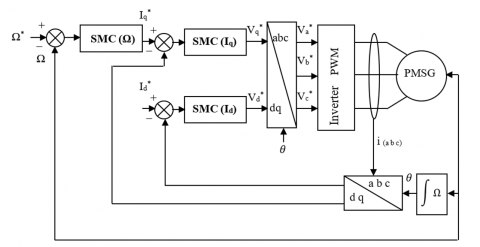
The block diagram of vector control by sliding mode is presented in Figure 7.
Figure 7. Block diagram of vector control by sliding mode
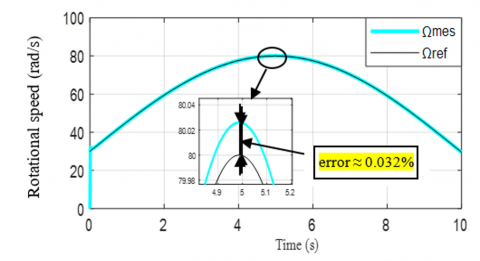
In this section, simulation results of kinetic energy storage, via a flywheel driven by the permanent magnet synchronous machine are presented. The reference rotational speed to impose for the storage system is determined from a desired power profile PD via RPPT optimization algorithm. The desired power oscillates between -600 W and +600 W. The rotational speed of the wheel is increasing and decreasing in motor (storage) and generator (power output) operating modes respectively. This speed follows its reference with an error of less than one percent as shown in Figure 8.
Figure 8. Rotational speed and its reference
The evolution of the power demand, and as expected follows the reference of the desired power with an error less than 1% (Figure 9). The positive and negative signs of the power correspond to the operating modes of the storage system. Motor (storage) and generator (restored energy).
Figure 9. Active power and its reference
The electromagnetic torque developed by the machine (Figure 10), is positive for motor operation and negative for the generator operation.
Figure 10. Electromagnetic torque waveform
The electromagnetic torque is controlled by the quadratic current component Iq. This is shown by the evolution of the current Iq which is the image of the torque as can be seen in Figure 11. The evolution of the voltage and the current of the same phase, over one period, in both operation modes are given in Figure 12 (motor, Figure 12(a), and generator Figure 12(b)).
Figure 11. Currents and their references in Park frame
Figure 12. Voltage and current waveforms: (a) Zoom on storage phase; (b) Zoom on restore phase
9.1 Presentation of the test bench
The studied system is implemented in the electrical engineering laboratory (G2eLAB) in Grenoble, France (Figure 13).
Figure 13. The physical components of the real-time test bench
The generation of flywheel torque is realized by a direct current machine. The flywheel with inertia $J_v$ is emulated by a DC machine, by adjusting the electromagnetic torque reference. According to the mechanical equation of the shaft direct current machine.
$J \frac{d \Omega}{d t}=T_{e m}+T_r$ (70)
By imposing the electromagnetic torque reference:
$T_{e m}=T_{e m_{-} r e f}=\left(J-J_v\right) \frac{d \Omega}{d t}$ (71)
Substituting Eq. (71) in Eq. (70), we obtain the mechanical equation that governs the mechanical operation of the flywheel.
$J_v \frac{d \Omega}{d t}=T_r$ (72)
Test bench consists of two essential parts:
1-(DC) whose torque is programmable via a DSP type TMS320F240. The whole is controlled by a TESTPOINT interface.
2-The machine: The machine used is of the permanent magnet synchronous type for which the stator is connected to the network via a power Bay which contains the AC/DC/AC power electronics interface, a connection transformer and the LC filters. The control of the whole is ensured by a DSPACE of type RTI1005.
We find in the complete bench the following elements:
-Mechanical part consisting of two machines with rigid coupling, the MCC which emulates the torque of the flywheel brought back to the shaft of the MS which is the reversible machine.
-The power bay associated with the DC motor consisting of a four quadrant chopper and its control, a DSP type TMS320F240, different sensor boards.
-The power bay associated with the synchronous motor: it contains two two-stage three-phase voltage inverters, a DSPACE system with a power PC, different sensor boards.
The network voltage before transformer (at the connection point of the synchronous machine to the EDF network) is about Veff=127V, 50Hz and the characteristics of the different components (inverter, grid, DC motor, PMSM) are given in the Tables 1-3.
Table 1. Bench characteristics inverter
|
Parameters |
Values |
|
Inverter power |
10kVA |
|
Standby time of the inverters |
0.00000325s |
|
Frequency PWM |
10kHz |
|
Inductance grid side line (Lf) |
0.003+0.002H |
|
Resistance of line grid rating (Rf) |
0.0521Ω |
|
DC bus capacitor Cbus |
0.0022F |
|
Line inductance on the machine side |
0.00036H |
|
Line resistance machine side |
0.01Ω |
|
Sampling frequency |
0.0001s |
Table 2. Internal parameters of the PMSM
|
Parameters |
Values |
|
Rated power |
6.9 kW |
|
Stator resistance (Rs) |
173,77.10-3 Ω |
|
Direct inductance (Ld) |
0,8524.10-3 H |
|
quadrature inductance (Lq) |
0,9515.10-3 H |
|
Rotor flux ϕr |
0.1112 Wb |
Table 3. Parameters of the DC machine
|
Parameters |
Values |
|
Rated power |
7.3 kW |
|
Rated speed |
3470 rpm |
|
Rated voltage |
310 V |
|
Rated torque |
24.8 Nm |
|
Armature resistance |
0.8 Ω |
|
Armature inductance |
0.0037 H |
9.2 Experimental results
The experimental results are presented below in three parts as follows:
9.2.1 Test with a desired power profile to validate the operation of the studied system as a motor/generator mode
In Figure 14, the machine rotation speed (Ω) follows exactly its reference (Ωref); It is of positive slope for the operation in storage mode and negative for the operating mode generator (restore). Also, the evolution of the quadrate component Iq is given, with positive or negative sign corresponding to the operating modes of the studied system, storage and destocking respectively. The active power waveform illustrates the direction of the power flow converted by the permanent magnet machine; the phase where the sign of the component of the current iq is positive corresponds to the storage mode, conversely, it corresponds to the mode of power restitution. Figure 15 shows the evolution of the supply voltage of the machine and the current flowing through it; depending on the operating modes, phase difference between current voltage varies between the zero and π/2 during the storage mode and between π/2 and π during generator operating mode (destocking) (Figure 16).
Figure 14. Speed (Ω) and its reference (Ωref); current Iq(A) and active power (Pm) waveforms
Figure 15. Voltage and current waveforms during storage phase
Figure 16 Voltage and current phase discharge
Figure 17 shows the phase current and voltage waveforms where the machine is decoupled from the flywheel, therefore the power absorbed is lost in the machine.
Figure 17. Voltage and current where the machine is decoupled from the flywheel
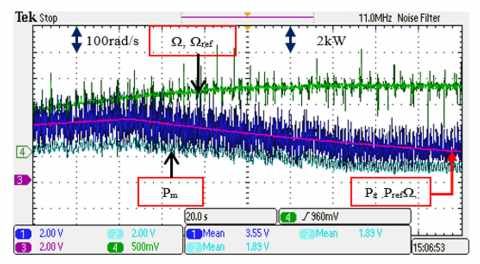
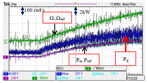
9.2.2 Test in motor mode, the measured power on the grid side
In this test, the reference power RPPT is compared to that measured on the grid side. The results obtained are given in Figures 18 and 19. The rotational speed of the machine (Ω) which faithfully follows its reference (Ωref). The electrical network provides the desired active power (Pg), this is clearly shown by the perfect tracking of its reference (Pref). It is also noted that the power absorbed by the stator is less than that provided by the network; this is due to losses in the static converter (Figure 18).
Figure 18. Speed and its reference Ω, Ωref, grid active power (Pg) and its reference RPPT, Pref; and machine active power Pm wave forms
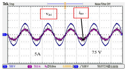
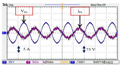
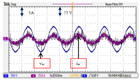
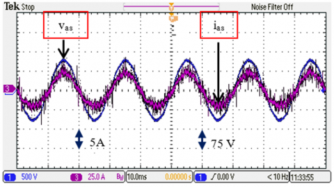
Figure 19 shows voltage and stator current of the same phase (vas), (ias) respectively. These wave forms clearly show that the storage system operates in motor mode (storage phase).
Figure 19. Voltage and current waveforms during storage phase
9.2.3 Test in motor mode, the measured power on the machine side
In this test, the reference power RPPT is compared with that measured on the machine side. In the obtained results, it can notice that the speed of rotation of the machine (Ω) coincides with its reference (Ωref), the active electric power (Pm) absorbed by the motor which perfectly follows its reference (Pref) and the active power provided by the network. It can be seen that the active power (Pg) supplied by the network is greater than that received by the machine. This is due to extra power provided by the network, and this power excess is dissipated in the power electronics bay. As a result, there is a risk of destabilizing the network (Figure 20).
Figure 20. Speed (Ω) and its reference (Ωref), grid active power (Pg), machine active power (Pm) and its reference RPPT (Pref) waveforms
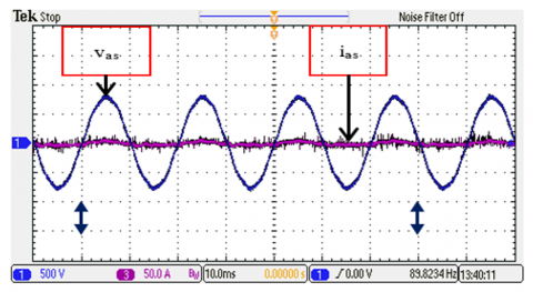
Figure 21 shows the voltage and the stator current of the same phase respectively, in which it can be seen clearly that the storage system works in motor mode (storage phase).
Figure 21. Voltage and current waveforms during storage phase
In this paper, an inertial storage system based on the synchronous permanent magnet machine is presented. The latter is connected to the micro-grid through a cascade of bidirectional power electronics. The PWM pulse width modulation technique is applied for the generation of the control signals in the power interface, the set is controlled by a field oriented control. The model of the studied system is implemented under the MATLAB Simulink environment and a calculation code is obtained. The simulation results are commented, and show that the studied system operates in motor and generator modes, storage and restore mode respectively, according to the need (reference of desired power). The mathematical model is validated experimentally.
The contribution in this article lies in one hand, in determining the reference speed from the desired power. In other hand the importance of the side where the power exchanged between the electrical grid and the system is measured. Indeed, it has been found by experiments that when measuring the power on the machine side, the electrical grid provides additional power, which is dissipated in the converter (storage phase). Therefore, the micro-network may be destabilized. While measuring the power of the grid side, the latter only provides the desired power. This fact contributes to the stability of the grid. This study offers several significant contributions:
⁕By accounting for static converter losses, our study provides a more realistic representation of the inertial storage system's behavior in actual grid scenarios. This is crucial for bridging the gap between theoretical models and practical implementation.
⁕Previous studies that did not consider static converter losses might have overestimated the efficiency of inertial storage systems. Our work contributes to a more accurate assessment of power exchange, helping researchers and practitioners understand the true performance of these systems in real-world applications.
⁕Understanding the impact of static converter losses allows for the development of optimized control strategies. Our study can potentially provide insights into adjusting control algorithms to mitigate these losses, improving the overall efficiency and performance of inertial storage systems in grid stabilization.
⁕By matching actual upstream or downstream power measurement points with a power reference, our study validates the reliability of network side power measurements. This contributes to the credibility of the measurements and strengthens the basis for asserting that the measurement of network side power indeed plays a significant role in contributing to network stability.
⁕Demonstrating the contribution of network side power measurement to network stability with a consideration of static converter losses has practical implications. This information can guide grid operators, policymakers, and system designers in making informed decisions about the integration and operation of inertial storage systems in the grid.
|
f |
Viscous friction coefficient |
|
id, iq |
Direct and quadrature of stator current |
|
Irec |
DC current |
|
J, Jv |
Motor and flywheel inertia |
|
Ld, Lq |
Direct and quadrature inductance |
|
PD |
Desired power |
|
Pg |
Grid active power |
|
Pm |
Machine active power |
|
r |
Radius of the flywheel |
|
Rs |
Stator resistance |
|
s |
Operational safety factor of the flywheel |
|
Tem |
Electromagnetic torque |
|
Tr |
Load torque |
|
Tf |
Friction torque |
|
vd, vq |
Direct and quadrate of stator voltages |
|
Vc, |
DC-link voltage |
|
Greek symbols |
|
|
Ωv |
Wheel rated speed capacitor |
|
Ωmec |
Mechanical speed |
|
Σ |
Tensile strength |
|
ρ |
Density of the material |
|
$\omega_e$ |
Stator angular velocities |
|
ϕr |
Roror flux |
|
Subscripts |
|
|
AC |
Alternative current |
|
DC |
Direct current |
|
DCM |
Direct current motor |
|
PMSG |
Permanent magnet synchronous generator |
|
RPPT |
Reference power point tracking |
|
VSI |
Voltage source inverter |
[1] Hassani, H., Zaouche, F., Rekioua, D., Belaid, S., Rekioua, T., Bacha, S. (2020). Feasibility of a standalone photovoltaic/battery system with hydrogen production. Journal of Energy Storage, 31: 101644. https://doi.org/10.1016/j.est.2020.101644
[2] Belaid, S., Rekioua, D., Oubelaid, A., Ziane, D., Rekioua, T. (2022). A power management control and optimization of a wind turbine with battery storage system. Journal of Energy Storage, 45: 103613. https://doi.org/10.1016/j.est.2021.103613
[3] Djamila, D.R., Toufik, P.R., Kassa Jr, I., Abdelmounaim, D.T. (2005). An approach for the modeling of an autonomous induction generator taking into account the saturation effect. International Journal of Emerging Electric Power Systems, 4(1): 1-23. https://doi.org/10.2202/1553-779X.1052
[4] Mebarki, N., Rekioua, T., Mokrani, Z., Rekioua, D. (2015). Supervisor control for stand-alone photovoltaic/hydrogen/battery bank system to supply energy to an electric vehicle. International Journal of Hydrogen Energy, 40(39): 13777-13788. https://doi.org/10.1016/j.ijhydene.2015.03.024
[5] Wang, X., Li, L., Palazoglu, A., El-Farra, N. H., Shah, N. (2018). Optimization and control of offshore wind systems with energy storage. Energy Conversion and Management, 173: 426-437. https://doi.org/10.1016/j.enconman.2018.07.079
[6] Ge, B., Wang, W., Bi, D., Rogers, C.B., Peng, F.Z., de Almeida, A.T., Abu-Rub, H. (2013). Energy storage system-based power control for grid-connected wind power farm. International Journal of Electrical Power & Energy Systems, 44(1): 115-122. https://doi.org/10.1016/j.ijepes.2012.07.021
[7] Shahmohammadi, A., Sioshansi, R., Conejo, A.J., Afsharnia, S. (2018). The role of energy storage in mitigating ramping inefficiencies caused by variable renewable generation. Energy Conversion and Management, 162: 307-320. https://doi.org/10.1016/j.enconman.2017.12.054
[8] Ayodele, T.R., Ogunjuyigbe, A.S.O. (2015). Mitigation of wind power intermittency: Storage technology approach. Renewable and Sustainable Energy Reviews, 44: 447-456. https://doi.org/10.1016/j.rser.2014.12.034
[9] Takarli, R., Amini, A., Khajueezadeh, M., et al. (2023). A comprehensive review on flywheel energy storage systems: Survey on electrical machines, power electronics converters, and control systems. IEEE Access, 38(2): 81224-81255. https://doi.org/10.1109/ACCESS.2023.3301148
[10] Arani, A.K., Karami, H., Gharehpetian, G.B., Hejazi, M.S.A. (2017). Review of Flywheel Energy Storage Systems structures and applications in power systems and microgrids. Renewable and Sustainable Energy Reviews, 69: 9-18. https://doi.org/10.1016/j.rser.2016.11.166
[11] Bolund, B., Bernhoff, H., Leijon, M. (2007). Flywheel energy and power storage systems. Renewable and Sustainable Energy Reviews, 11(2): 235-258. https://doi.org/10.1016/j.rser.2005.01.004
[12] Belfedhal, S., Berkouk, E.M., Meslem, Y., Soufi, Y. (2012). Modeling and control of wind power conversion system with a flywheel energy storage system and compensation of reactive power. International Journal of Renewable Energy Research, 2(3): 528-534.
[13] Jia, Y., Wu, Z., Zhang, J., Yang, P., Zhang, Z. (2022). Control strategy of flywheel energy storage system based on primary frequency modulation of wind power. Energies, 15(5): 1850. https://doi.org/10.3390/en15051850
[14] Vafakhah, B., Masiala, M., Salmon, J., Knight, A. (2008). Emulation of flywheel energy storage systems with a PMDC machine. In 2008 18th International Conference on Electrical Machines, Vilamoura, Portugal, pp. 1-6. https://doi.org/10.1109/ICELMACH.2008.4799935
[15] Gamboa, P., Pinto, S.F., Silva, J.F., Margato, E. (2008). A flywheel energy storage system with matrix converter controlled permanent magnet synchronous motor. In 2008 18th International Conference on Electrical Machines, Vilamoura, Portugal, pp. 1-5. https://doi.org/10.1109/ICELMACH.2008.4799861
[16] Talebi, S., Nikbakhtian, B., Toliyat, H.A. (2007). A novel algorithm for designing the PID controllers of high-speed flywheels for traction applications. In 2007 IEEE Vehicle Power and Propulsion Conference, Arlington, TX, USA, pp. 574-579. https://doi.org/10.1109/VPPC.2007.4544188
[17] Idjdarene, K., Rekioua, D., Rekioua, T., Tounzi, A. (2011). Wind energy conversion system associated to a flywheel energy storage system. Analog Integrated Circuits and Signal Processing, 69: 67-73. https://doi.org/10.1007/s10470-011-9629-2
[18] Elkomy, A., Huzayyin, A., Abdo, T.M., Adly, A.A., Yassin, H.M. (2017). Enhancement of wind energy conversion systems active and reactive power control via flywheel energy storage systems integration. In 2017 Nineteenth International Middle East Power Systems Conference (MEPCON), Cairo, Egypt, pp. 1151-1156. https://doi.org/10.1109/MEPCON.2017.8301327
[19] Xu, K., Guo, Y., Lei, G., Zhu, J. (2023). A review of flywheel energy storage system technologies. Energies, 16(18): 6462. https://doi.org/10.3390/en16186462
[20] Aissou, R., Rekioua, T., Rekioua, D., Tounzi, A. (2016). Application of nonlinear predictive control for charging the battery using wind energy with permanent magnet synchronous generator. International Journal of Hydrogen Energy, 41(45): 20964-20973. https://doi.org/10.1016/j.ijhydene.2016.05.249
[21] R Jr, D.A. (2004). A superconducting high-speed flywheel energy storage system. Physica C, 408: 930-931. https://doi.org/10.1016/j.physc.2004.03.168
[22] Bolund, B., Bernhoff, H., Leijon, M. (2007). Flywheel energy and power storage systems. Renewable and Sustainable Energy Reviews, 11(2): 235-258. https://doi.org/10.1016/j.rser.2005.01.004
[23] Aissou, R., Rekioua, T., Rekioua, D., Tounzi, A. (2016). Robust nonlinear predictive control of permanent magnet synchronous generator turbine using DSPACE hardware. International Journal of Hydrogen Energy, 41(45): 21047-21056. https://doi.org/10.1016/j.ijhydene.2016.06.109
[24] Mohammedi, A., Rekioua, D., Rekioua, T., Bacha, S. (2016). Valve Regulated Lead Acid battery behavior in a renewable energy system under an ideal Mediterranean climate. International Journal of Hydrogen Energy, 41(45): 20928-20938. https://doi.org/10.1016/j.ijhydene.2016.05.087
[25] Iman-Eini, H., Frey, D., Bacha, S., Boudinet, C., Schanen, J.L. (2019). Evaluation of loss effect on optimum operation of variable speed micro-hydropower energy conversion systems. Renewable Energy, 131: 1022-1034. https://doi.org/10.1016/j.renene.2018.07.122
[26] Guo, B., Bacha, S., Alamir, M., Mohamed, A., Boudinet, C. (2019). LADRC applied to variable speed micro-hydro plants: Experimental validation. Control Engineering Practice, 85: 290-298. https://doi.org/10.1016/j.conengprac.2019.02.008
[27] Rekioua, D., Rekioua, T. (2009). DSP-controlled direct torque control of induction machines based on modulated hysteresis control. In 2009 International Conference on Microelectronics - ICM, Marrakech, Morocco, pp. 378-381. https://doi.org/10.1109/ICM.2009.5418603
[28] Idjdarene, K., Rekioua, D., Rekioua, T., Tounzi, A. (2007). Control strategies for an autonomous induction generator taking the saturation effect into account. In 2007 European Conference on Power Electronics and Applications, Aalborg, Denmark, pp. 1-10. https://doi.org/10.1109/EPE.2007.4417591
[29] Tadjine, K., Rekioua, D., Belaid, S., Rekioua, T., Logerais, P.O. (2022). Design, modeling and optimization of hybrid photovoltaic/wind turbine system with battery storage: Application to water pumping. Mathematical Modelling of Engineering Problems, 9(3): 655-667. https://doi.org/10.18280/mmep.090312
[30] Errami, Y., Ouassaid, M., Maaroufi, M. (2015). Optimal power control strategy of maximizing wind energy tracking and different operating conditions for permanent magnet synchronous generator wind farm. Energy Procedia, 74: 477-490. https://doi.org/10.1016/j.egypro.2015.07.732