Aruna Devi Ramsankar![]() | Anitha Krishnamoorthy*
| Anitha Krishnamoorthy*![]()
© 2024 The authors. This article is published by IIETA and is licensed under the CC BY 4.0 license (http://creativecommons.org/licenses/by/4.0/).
OPEN ACCESS
In this study, we propose to calculate multiple metric dimensions using different distances. This approach can lead to the implementation of dimensionality reduction techniques for a specific information system. By combining traditional graph theory with rough set theory, which involves using uncertain or ambiguous data, we can construct a rough graph to depict the relationships between attributes. The rough graph is constructed based on the rough membership function, which defines the link between the conditional and decision features. By utilizing degree-based metric dimensions, we can identify and remove inconsistent features from the information system. If each vertex’s vector of distances from the other vertices in the set is unique, it means that the set of vertices can fully determine the graph. The metric dimension, which represents the smallest cardinality of a resolving set, plays a role in facilitating navigation and aiding in location determination within the graph.
rough graph, rough membership function, reduct, rough metric dimension
The integration of rough set theory with graph theory resulted in the emergence of a novel concept called rough graph. This concept combines the principles of rough set theory, which deals with uncertainty and vagueness in the data, with the established framework of graph theory [1-6]. The utilization of rough sets across various domains is examined [7-15]. The formulation of rough graphs involves the examination of graphs within the framework of rough sets, providing a means to depict networks characterized by uncertain information. He Tong and Shi introduced the concept of rough graph in 2006, placing emphasis on the edge set. In the same year, He et al expanded on this concept by introducing a weighted rough graph [16-18], where class weights were assigned to the edge equivalence class [eab]R. They also developed a generalized algorithm based on the Kruskal algorithm to obtain the optimal tree within a weighted rough graph. In 2007, the rough graph was further defined with the introduction of the double universe of discourse [19]. Several algorithms from classical graph theory can be adapted for application in rough graphs. We leverage the Dijkstra algorithm, originally designed for exploring the shortest path in graphs, to develop a specialized shortest path algorithm tailored for weighted rough graphs. Liang et al. introduced an edge rough graph that utilizes the edge approximation space, providing a means to compute the clique number of a graph [20]. In order to determine the accuracy of a rough graph, He T used the edge precision and conducted a comparative study using the concepts of rough equality and rough similarity degrees. This study also introduced different representation forms for the rough graph [21, 22].
Researchers have explored the integration of the rough graph with various soft computing concepts, such as fuzzy logic and neutrosophic theory [23]. By combining the rough graph with these approaches, it becomes possible to handle uncertainties and vagueness in a more comprehensive manner, enhancing the representation and analysis of relationships between items or entities. In a related development, Bibin et al proposed a novel idea to construct vertex rough graphs by dividing the vertex set [24]. This approach involves partitioning the vertices into subsets, which enables a more refined representation of relationships within the graph.
Wang et al investigates the transitive closure and minimum equivalent graph operations, preserving the path information of a directed graph. Specifically, it employs the minimum equivalent graph and transitive closure to approximate a directed graph, constructing a Path Information-based Rough Directed Graph (PIRDG) model. To overcome this constraint, the paper introduces three graph reducts by treating each directed graph as a PIRDG. It examines the relationship between these reducts and proposes a method to identify an optimal graph reduct [25]. Akram et al address a specified multi-criteria shortest path problem in a weighted connected directed network, where the associated edge weights are expressed as rough variables to handle imprecision. Two distinct approaches have been presented to ascertain the optimal path(s) for the given problem [26]. Anitha and Aruna Devi employed rough membership functions to construct rough graphs, and subsequently conducted an analysis of metric dimension within approximation-based rough graphs [27, 28]
The applications of rough graphs span a wide range of fields. In graph mining, rough graphs are utilized to extract valuable insights and patterns from complex networks. Nithya and Anitha introduced the concept of labeling in rough graphs, accompanied by its applications in Wireless Sensor Networks [29-31]. The rough graph framework provides a powerful tool for analyzing the intricate relationships and structures present in various types of networks, such as social networks or biological networks. In complex networks analysis [32], rough graphs contribute to understanding the underlying connectivity and patterns within the network. Connecting certain metropolitan networks together presents a modeling problem by expressing one directed graph through another. There are two types of simulations available: univocal and multivocal. The concepts of fragment and atom are important to our analysis of connectedness in the virtual digraph. This comprises a different evaluation of k-connectivity. A unique proposal in this study is the inclusion of the rough set technique in (bi) digraph, which greatly improves the evaluation of k-connectivity [33]. By applying rough graph techniques, researchers can uncover hidden relationships and gain a deeper understanding of the network’s structure, dynamics, and properties. Relationship analysis is another important area where rough graphs find application. By representing relationships using rough graphs, it becomes possible to analyze and quantify the strength, similarity, or dissimilarity between entities or items. This can be useful in various domains, including customer relationship management, recommender systems, or social network analysis. The rough membership function structure minimizes inter-node distances, and the LOA-LSTM algorithm for routing attains elevated throughput and energy efficiency [34, 35]. Data mining is yet another domain where rough graphs prove beneficial. By employing rough graph-based techniques, it becomes possible to extract useful knowledge and insights from large and complex datasets. Social media network analysis (SMNA) is a fascinating field that applies the tools and concepts of network analysis to the complex world of online social networks like Facebook, Twitter, and Instagram. Rough set theory-based pattern identification has been done using social media data. The rough graph framework provides a flexible and powerful means to analyze and explore data, facilitating tasks such as clustering, classification, and anomaly detection [36]. Solving problems with DRFG connectivity that are difficult to solve using fuzzy graphs. In order to analyze trade deficits in Asian developing countries during the COVID-19 pandemic, the paper's conclusion looks into the trade network in developing countries using DRF-edge analysis [37]. This paper presents the introduction of the degree-based metric dimension. The second section provides an overview of the fundamental concepts related to the rough graph. In the third section, we introduce the concept of degree-based metric dimension and derive several results. This is followed by examples illustrating the degree-based metric dimension of specific graphs. Finally, the fourth section concludes the paper with some remarks.
2.1 Definition
Suppose we are given a set of objects $\mathfrak{U}$ called the universe and an indiscernibility relation $\mathfrak{B} \subseteq \mathfrak{U}$, representing our lack of knowledge about elements of $\mathfrak{U}$. Let $\mathfrak{X}$ be a subset of $\mathfrak{U}$. The set $\mathfrak{X}$ with respect to $\mathfrak{R}$ :
$\mathfrak{B}$ - lower approximation of $\mathfrak{X}$
$\mathfrak{B}_*(\mathfrak{X})=\{\mathfrak{x} \in \mathfrak{U}: \mathfrak{B}(\mathfrak{x}) \subseteq \mathfrak{X}\}$
$\mathfrak{B}$ - upper approximation of $\mathfrak{X}$
$\mathfrak{B}^*(\mathfrak{X})=\{\mathfrak{x} \in \mathfrak{U}: \mathfrak{B}(\mathfrak{x}) \cap \mathfrak{X} \neq \emptyset\}$
The process of reducing an information system such that the set of attributes of the reduced information system is independent and no attribute can be eliminated further without losing some information from the system, the result is known as reduct. Rough sets can also be defined using a rough membership function, defined:
$\mu_{\mathfrak{x}}^{\mathfrak{B}}(\mathfrak{x})=\frac{|\mathfrak{X} \cap \mathfrak{B}(\mathfrak{x})|}{|\mathfrak{B}(\mathfrak{x})|}$
where, $\mu_x^{\mathfrak{B}}(\mathfrak{x}) \in[0,1]$.
2.2 Definition [2]
An information system is converted to a rough graph by taking the set of all objects as $\mathfrak{U}$ and the attribute set as $\mathfrak{P P}$ which creates the corresponding vertex set $\mathfrak{B}=$ $\left\{\mathfrak{v}_1, \mathfrak{v}_2, \ldots, \mathfrak{v}_{|\mathfrak{B}|}\right\}$ associated with an edge set $\mathfrak{E}=\cup \mathfrak{e}_{\mathfrak{f}}\left(\mathfrak{v}_{\mathfrak{i}}, \mathfrak{v}_{\mathfrak{j}}\right)$. This $\mathfrak{E}$ can be decomposed into different equivalence classes $[\mathfrak{e}]_{\mathfrak{B}}$.
For any subgraph $\mathfrak{I}=(\mathfrak{B}, \mathfrak{Y})$, where $\mathfrak{B} \subseteq \mathfrak{B}, \mathfrak{Y} \subseteq \mathfrak{E}$, graph $\mathfrak{I}$ is called $\mathfrak{B}$-definable graph or $\mathfrak{B}$-exact graph if $\mathfrak{Y}$ is the union of some $[\mathfrak{e}]_{\mathfrak{B}}$. Conversely, graph $\mathfrak{I}$ is called $\mathfrak{B}$-undefinable graph or $\mathfrak{B}$ - rough graph, two exact graphs $\mathfrak{B}(\mathfrak{T})_*=\left(\mathfrak{B}, \mathfrak{B}(\mathfrak{Y})_*\right)$ and $\mathfrak{B}(\mathfrak{T})^*=\left(\mathfrak{B}, \mathfrak{B}(\mathfrak{Y})^*\right)$ can be used to define it approximately, where,
$\begin{gathered}\mathfrak{B}(\mathfrak{Y})_*=\left\{\mathfrak{e} \in \mathfrak{E}:[\mathfrak{e}]_{\mathfrak{B}} \subseteq \mathfrak{V}\right\} \\ \mathfrak{B}(\mathfrak{Y})^*=\left\{\mathfrak{e} \in \mathfrak{E}:[\mathfrak{e}]_{\mathfrak{B}} \cap \mathfrak{Y} \neq \emptyset\right\}\end{gathered}$
The graphs $\mathfrak{B}(\mathfrak{T})_*$ and $\mathfrak{B}(\mathfrak{T})^*$ are called $\mathfrak{B}-$ lower and $\mathfrak{B}$ - upper approximate graphs of $\mathfrak{T}$. The pair of graphs $\left(\mathfrak{B}(\mathfrak{T})_*, \mathfrak{B}(\mathfrak{T})^*\right)$ is called $\mathfrak{B}$ - rough graph. The set $\mathfrak{D H}_{\mathfrak{B}}(\mathfrak{Y})=$ $\mathfrak{B}(\mathfrak{Y})^*-\mathfrak{B}(\mathfrak{Y})_*$ is called the $\mathfrak{B}$ - boundary of edge set $\mathfrak{Y}$ of $\mathfrak{T}$.
2.3 Definition [3]
Given the universe graph $\mathfrak{U}=(\mathfrak{V}, \mathfrak{E}), \mathfrak{V}=\left\{\mathfrak{v}_1, \mathfrak{v}_2, \ldots, \mathfrak{v}_{\mathfrak{n}}\right\}$, $\mathfrak{E}=U \mathfrak{e}_{\mathfrak{f}}\left(\mathfrak{v}_{\mathfrak{i}}, \mathfrak{y}_{\mathfrak{i}}\right) \forall \mathfrak{e} \in \mathfrak{E}$, let the mapping $\omega: \mathfrak{e} \rightarrow \omega(\mathfrak{e})$, the real number $\omega(\mathfrak{e})$ is called the edge weight of $\mathfrak{e}$. $\left(\left[\mathfrak{e}_{\mathfrak{u v}}\right]_{\mathfrak{B}}\right)=$ $\mathfrak{f}(\omega(\mathfrak{e}))$ is called the class weight of edge equivalence class $\left[\mathfrak{e}_{\mathfrak{u v}}\right]_{\mathfrak{B}}$, where $\mathfrak{e} \in\left[\mathfrak{e}_{\mathfrak{u v}}\right]_{\mathfrak{B}},\left[\mathfrak{e}_{\mathfrak{u v}}\right]_{\mathfrak{B}}$ is the edge equivalence class between the vertex $\mathfrak{u}$ and vertex $\mathfrak{v}$ respect to attribute $\mathfrak{B}$, with respect to $\mathfrak{f}$.
The weighted rough graph is pair of graphs $\mathfrak{T}=$ $\mathfrak{B}(\mathfrak{T}), \overline{\mathfrak{B}}(\mathfrak{T})$ with the class weight of their edge equivalence class.
2.4 Definition [6]
Let $\mathcal{A}=(\mathfrak{K}, \mathfrak{B})^{\mathrm{e}}$ be an approximation space for edges. Given an edge subset $\mathfrak{Y} \subseteq \mathfrak{E}(\mathfrak{K})$, we define lower and upper approximation of $\mathfrak{Y}$ in $\mathcal{A}$, denoted by:
$\begin{gathered}\mathfrak{Q}_*(\mathfrak{Y})=\left\{\mathfrak{y} \in \mathfrak{E}(\mathfrak{K}) \mid \mathfrak{I}_{\mathfrak{Q}}(\mathfrak{y}) \subseteq \mathfrak{V}\right\} \\ \mathfrak{Q}^*(\mathfrak{Y})=\left\{\mathfrak{y} \in \mathfrak{E}(\mathfrak{K}) \mid \mathfrak{J}_{\mathfrak{Q}}(\mathfrak{y}) \cap \mathfrak{Y} \neq \varphi\right\}\end{gathered}$
where, $\widetilde{J}_{\mathfrak{Q}}(\mathfrak{y})$ denotes the edge set $\{\mathfrak{y} \in \mathfrak{E}(\mathfrak{K}) \mid(\mathfrak{y}, \mathfrak{z}) \in \mathfrak{Q}\}$
2.5 Definition [13]
$\mathfrak{B}$ - vertex rough graph is defined in terms of two exact graphs $\mathfrak{B}_*(\mathfrak{T})=\left(\mathfrak{B}_*(\mathfrak{B}), \mathfrak{B}_*(\mathfrak{Y})\right)$ and $\mathfrak{B}^*(\mathfrak{T})=\left(\mathfrak{B}^*(\mathfrak{B}), \mathfrak{B}^*(\mathfrak{V})\right)$, where,
$\begin{aligned} & \mathfrak{B}_*(\mathfrak{M})=\left\{\mathfrak{v} \in \mathfrak{B}:[\mathfrak{p}]_{\mathfrak{B}} \subseteq \mathfrak{M}\right\} \\ & \mathfrak{B}^*(\mathfrak{M})=\left\{\mathfrak{v} \in \mathfrak{B}:[\mathfrak{v}]_{\mathfrak{B}} \cap \mathfrak{M} \neq \varnothing\right\} \\ & \mathfrak{B}_*(\mathfrak{V})=\left\{\left(\mathfrak{v}_{\mathfrak{i}}, \mathfrak{b}_{\mathfrak{i}}\right) \in \mathfrak{E}: \mathfrak{v}_{\mathfrak{i}}, \mathfrak{p}_{\mathfrak{i}} \in[\mathfrak{p}]_{\mathfrak{B}} \text { for some } \mathfrak{v} \in \mathfrak{B}_*(\mathfrak{B})\right\} \\ & \mathfrak{B}^*(\mathfrak{Y})=\left\{\begin{array}{c}\left.\left(\mathfrak{v}_{\mathfrak{i}}, \mathfrak{v}_{\mathfrak{i}}\right) \in \mathfrak{E}: \mathfrak{v}_{\mathfrak{i}}, \in\left[\mathfrak{v}_{\mathfrak{i}}\right]_{\mathfrak{B}} \text { and }\left[\mathfrak{v}_{\mathfrak{i}}\right]_{\mathfrak{B}} \cap \mathfrak{V} \neq \varnothing\right) \\ \mathfrak{v}_{\mathfrak{i}} \in\left[\mathfrak{v}_{\mathfrak{i}}\right]_{\mathfrak{B}} \text { and }\left[\mathfrak{v}_{\mathfrak{i}}\right]_{\mathfrak{B}} \cap \neq \varnothing\end{array}\right. \\ & \end{aligned}$
$\mathfrak{B}$-lower approximate graph of $\mathfrak{I}$ and $\mathfrak{B}$-upper approximate graph of $\mathfrak{I}$ are the graphs $\mathfrak{B}_*(\mathfrak{I})$ and $\mathfrak{B}^*(\mathfrak{I})$ respectively. $\mathfrak{B}$ vertex rough graph is a pair of graphs $\left(\mathfrak{B}_*(\mathfrak{I}), \mathfrak{B}^*(\mathfrak{I})\right)$.
2.6 Definition [37]
A fuzzy rough digraph on a non empty set $\mathfrak{U}$ is a four ordered tuple $\mathfrak{G}=(\mathfrak{U}, \mathfrak{T} \mathfrak{A}, \mathfrak{P}, \mathfrak{H P})$, where,
$\begin{gathered}(\underline{\mathfrak{G}}(\mathfrak{P}))(\mathfrak{x} \mathfrak{z}) \leq \min \{\underline{\mathfrak{T}}(\mathfrak{H})(\mathfrak{x}), \underline{\mathfrak{T}}(\mathfrak{H})(\mathfrak{z})\} \\ (\overline{\mathfrak{H}}(\mathfrak{P}))(\mathfrak{x}) \leq \min \{\mathfrak{I}(\mathfrak{U})(\mathfrak{x}), \overline{\mathfrak{T}}(\mathfrak{H})(\mathfrak{z})\}, \forall \mathfrak{x}_{\mathfrak{Z}} \in \mathfrak{P}^*\end{gathered}$
2.7 Definition [15]
Let $\Re=\{\mathfrak{B}, \mathfrak{E}, \omega\}$ be a triple consisting of non-empty set $\mathfrak{B}=\left\{\mathfrak{v}_1, \mathfrak{v}_2, \ldots, \mathfrak{v}_{\mathfrak{H}}\right\}=\mathfrak{U}$ where $\mathfrak{U}$ is a universe, $\mathfrak{E}=$ $\left\{e_1, e_2, \ldots, e_m\right\}$ be an edge set for $\mathfrak{B}$ and $\omega$ be a function $\omega: \mathfrak{B} \rightarrow$ $[0,1]$. A rough graph is defined as,
$\mathfrak{N}\left(\mathfrak{v}_{\mathfrak{i}}, \mathfrak{v}_{\mathfrak{j}}\right)=\left\{\begin{array}{l}\text { if } \max \left(\omega_{\mathfrak{G}}^{\mathfrak{Y}}\left(\mathfrak{v}_{\mathfrak{i}}\right), \omega_{\mathfrak{G}}^{\mathfrak{Y}}\left(\mathfrak{v}_{\mathfrak{i}}\right)\right)>0, \mathfrak{v}_{\mathfrak{i}} \mathfrak{p}_{\mathfrak{i}} \text { exists } \\ \text { if } \max \left(\omega_{\mathfrak{F}}^{\mathfrak{Y}}\left(\mathfrak{v}_{\mathfrak{i}}\right), \omega_{\mathfrak{F}}^{\mathfrak{Y}}\left(\mathfrak{v}_{\mathfrak{i}}\right)\right)=0, \quad \text { no edge }\end{array}\right.$
Some of the properties of rough graph
In this section we have defined some various degree based metric dimension and theorems based on the degree based metric dimension. Let $\Re$ be a simple rough graph with the vertex set $\mathfrak{B}=\left\{\mathfrak{v}_1, \mathfrak{v}_2, \ldots, \mathfrak{v}_{\mathfrak{n}}\right\}$ and the edge set $\mathfrak{E}=$ $\left\{\mathfrak{e}_1, \mathfrak{e}_2, \ldots, \mathfrak{e}_m\right\} . \mathfrak{d}(\mathfrak{a}, \mathfrak{b})$ gives the distance between $\mathfrak{a}$ and $\mathfrak{b}$, which is the length of the shortest path between $\mathfrak{a}$ and $\mathfrak{b}$, where $\mathfrak{a}$ and $\mathfrak{b}$ are vertices.
3.1 Definition
A vertex’s degree is determined by the number of edges that occur at that vertex. The degree-based distance between a and b is defined as:
$\mathfrak{D} \mathfrak{D}=\Delta(\mathfrak{a}) \Delta(\mathfrak{b}) \mathfrak{D}(\mathfrak{a}, \mathfrak{b})$
A set of vertices is considered to resolve a given graph when each vertex is uniquely determined by its degree-based distance to other vertices. If a vertex $\mathfrak{x} \in \mathfrak{B}(\mathfrak{G})$ resolves a pair of vertices $\mathfrak{a}, \mathfrak{b} \in \mathfrak{B}(\mathfrak{b})$ by satisfying the condition $\mathfrak{d}_\delta(\mathfrak{a}, \mathfrak{x}) \neq$ $\mathfrak{D}_\delta(\mathfrak{b}, \mathfrak{x})$, then the set of vertices $\mathfrak{A} \subseteq \mathfrak{B}(\mathfrak{G})$ is a resolving set for $\mathfrak{G}$. A resolving set ensures that every pair of distinct vertices in $\mathfrak{G}$ is uniquely determined by at least one vertex in $\mathfrak{A}$. The minimum cardinality of such a resolving set is termed the metric basis of $\mathfrak{G}$, and its size, denoted as $|\mathfrak{U}|$, is known as the degree-based metric dimension, represented as $\beta_{\mathfrak{D D}}(\mathfrak{G})$.
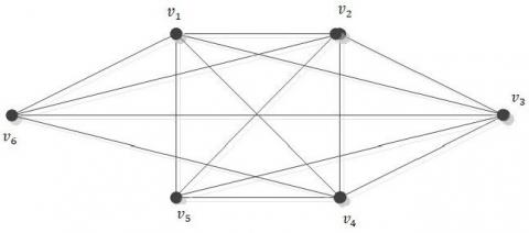
Example 1. Take into account the graph illustrated in Figure 1, where, $\mathfrak{B}(\mathfrak{G})=\left\{\mathfrak{v}_1, \mathfrak{v}_2, \mathfrak{v}_3, \mathfrak{v}_4, \mathfrak{v}_5, \mathfrak{v}_6\right\}$ and $(\mathfrak{5})=$ $\left\{\mathfrak{e}_1, \mathfrak{e}_2, \ldots, \mathfrak{e}_{14}\right\}$ denote the vertex and edge sets of $\mathfrak{G}$. In this context, the set $\mathfrak{U}=\left\{\mathfrak{v}_1, \mathfrak{v}_2, \mathfrak{v}_3, \mathfrak{v}_5\right\}$ serves as the metric basis or resolving set for $\mathfrak{5}$. The representation of all vertices concerning $\mathfrak{U}$ is provided in Table 1.
Figure 1. Rough graph
Table 1. Distance vector of G w.r.t A
|
$\mathfrak{d}$ (…) |
$\mathfrak{v}_1$ |
$\mathfrak{v}_2$ |
$\mathfrak{v}_3$ |
$\mathfrak{v}_4$ |
$\mathfrak{v}_5$ |
$\mathfrak{v}_6$ |
|
$\mathfrak{A}=\left\{\mathfrak{v}_1, \mathfrak{v}_2, \mathfrak{v}_3, \mathfrak{v}_5\right\}$ |
(0,5,5,5) |
(5,0,5,5) |
(5,5,0,5) |
(5,5,5,0) |
(4.5,4.5, 4.5,0) |
(4.5,4.5, 4.5,4.5) |
Theorem 1. The path rough graph has a degree distance metric dimension of 1.
Proof. The degree-based distance is defined as:
$\frac{1}{2}\left(\mathfrak{d}\left(\mathfrak{v}_1, \mathfrak{v}_2\right)\left(\delta\left(\mathfrak{v}_1\right)+\delta\left(\mathfrak{v}_2\right)\right)\right)=\mathfrak{b}_\delta\left(\mathfrak{v}_1, \mathfrak{v}_2\right)$
In the path rough graph, the initial and terminal vertices will have a degree of 1 each, while the degrees of the other vertices will be 2.
The degree distance vector representation of R with respect to A is segmented into two distinct cases.
Case (i): If $\mathfrak{A}=\left\{\mathfrak{v}_1\right\}$, then $\beta_\delta\left(\mathfrak{P}_n\right)=1$, for $\mathfrak{n}=4,6,8$, $10, \ldots, 2 \mathfrak{n}$.
The vector representation of $\mathfrak{G}$ w.r.t $\mathfrak{A}$ will be:
$\mathfrak{r}\left(\mathfrak{v}_\alpha \mid \mathfrak{A}\right)\left\{\begin{array}{cc}0, & \text { when } \alpha=1 \\ 2, & \text { when } \alpha=2 \\ 4, & \text { when } \alpha=3 \\ \cdot \\ \cdot \\ \mathfrak{n}-1, & \text { when } \alpha=\mathfrak{n}\end{array}\right.$
∴ The resolving set $\mathfrak{P}_n(\mathfrak{n}=4,6,8, \ldots, 2 \mathfrak{n})$ will be $\mathfrak{v}_1$.
$\beta_\delta\left(\mathfrak{P}_n\right)=1$ for $\mathfrak{n}=4,6, \ldots, 2 \mathfrak{n}$
Case (ii): If $\mathfrak{A}=\left\{\mathfrak{v}_2\right\}$, then $\beta_\delta\left(\mathfrak{P}_n\right)=1$, for $\mathfrak{n}=5,7,9, \ldots, 2 \mathfrak{n}+1$.
The vector representation of $\mathfrak{G}$ w.r.t $\mathfrak{A}$ will be:
$\mathfrak{r}\left(\mathfrak{v}_\alpha \mid \mathfrak{U}\right)\left\{\begin{array}{cc}2, & \text { when } \alpha=1 \\ 0, & \text { when } \alpha=2 \\ 4, & \text { when } \alpha=3 \\ & \cdot \\ & \cdot \\ \mathfrak{n}+2 \mathfrak{m}+1, & \text { when } \alpha=\mathfrak{n} \text { and } \mathfrak{m}=0,1,2, \ldots\end{array}\right.$
∴ The resolving set $\mathfrak{P}_n(\mathfrak{n}=5,7, \ldots, 2 \mathfrak{n}+1)$ will be $\mathfrak{v}_2$.
∴ $\beta_\delta\left(\mathfrak{P}_{\mathfrak{n}}\right)=1$ for $\mathfrak{n}=5,7, \ldots, 2 \mathfrak{n}+1(\mathfrak{n} \geq 5)$.
Example 2. In Figure 2, consider $\mathfrak{P}_7$ with vertex set $\left\{\mathfrak{v}_1, \mathfrak{v}_2, \ldots, \mathfrak{v}_7\right\}$ and edge set $\left\{\mathfrak{e}_1, \mathfrak{e}_2, \ldots, \mathfrak{e}_6\right\}$. The resolving set for $\mathfrak{P}_7$ is $\left\{\mathfrak{v}_2\right\}$. The degree-distance representation vector for $\mathfrak{P}_7$ with respect to $\mathfrak{A}$ will be provided in Table 2 .
Table 2. Degree-distance vector $\mathfrak{P}_7$ w.r.t $\mathfrak{A}$
|
$\mathfrak{d}$ (…) |
$\mathfrak{v}_1$ |
$\mathfrak{v}_2$ |
$\mathfrak{v}_3$ |
$\mathfrak{v}_4$ |
$\mathfrak{v}_5$ |
$\mathfrak{v}_6$ |
$\mathfrak{v}_7$ |
|
$\mathfrak{A}=\left\{ \mathfrak{v}_2 \right\}$ |
2 |
0 |
4 |
8 |
12 |
16 |
10 |
Figure 2. Rough path with 7 vertices P7
Theorem 2. The cycle rough graph has a degree distance metric dimension of 2.
Proof. The degree-distance is $\frac{1}{2}\left(\mathfrak{D}\left(\mathfrak{v}_1, \mathfrak{v}_2\right)\left(\delta\left(\mathfrak{v}_1\right)+\delta\left(\mathfrak{v}_2\right)\right)\right)$, where, $\mathfrak{v}_1, \mathfrak{v}_2, \ldots, \mathfrak{v}_{\mathfrak{n}} \in \mathfrak{C}_{\mathfrak{n}}$.
In the cycle rough graph, every vertex has a degree of 2, as it is a 2-regular rough graph. The degree distance vector representation of $\mathfrak{C}_n$ with respect to $\mathfrak{A}$ will involve 2 distinct cases.
Case (i): If $\left\{\mathfrak{v}_1, \mathfrak{v}_2\right\}=\mathfrak{A}$, then $\beta_\delta\left(\mathfrak{C}_{\mathfrak{n}}\right)=2$ for $\mathfrak{n}=$ $6,7, \ldots, \mathfrak{n}$ and $\mathfrak{n}=4$. Since $\mathfrak{m}=4$, the vector representation for $\mathfrak{C}_{\mathfrak{n}}$ w.r.t $\mathfrak{A}$ will be:
$r\left(\mathfrak{v}_\alpha \mid \mathfrak{H}\right)\left\{\begin{array}{cc}(0, \mathfrak{m}), & \text { when } \alpha=1 \\ (\mathfrak{m}, 0), & \text { when } \alpha=2 \\ & \cdot \\ & \cdot \\ (2 \mathfrak{m}, 3 \mathfrak{m}), & \text { when } \alpha=\mathfrak{n}-1 \\ (\mathfrak{m}, 2 \mathfrak{m}), & \text { when } \alpha=\mathfrak{n}\end{array}\right.$
∴$\beta_\delta\left(\mathfrak{C}_{\mathfrak{n}}\right)=2$ for $\mathfrak{n}=6,7,8, \ldots$ and $\mathfrak{n}=4$.
Case (ii): For $\mathfrak{C}_3$ and $\mathfrak{C}_5$, the vector representation is given as:
$r\left(\mathfrak{v}_\alpha \mid \mathfrak{H}\right)=\left\{\begin{array}{l}(0, \mathfrak{m}), \text { when }=1 \\ (\mathfrak{m}, 0), \text { when }=2 \\ (\mathfrak{m}, \mathfrak{m}), \text { when }=3\end{array}\right.$
For $\mathfrak{C}_5$,
$\mathfrak{r}\left(\mathfrak{v}_\alpha \mid \mathfrak{U}\right)=\left\{\begin{array}{cc}(0, \mathfrak{m}), & \text { when } \alpha=1 \\ (\mathfrak{m}, 0), & \text { when } \alpha=2 \\ (2 \mathfrak{m}, \mathfrak{m}), & \text { when } \alpha=3 \\ (2 \mathfrak{m}, 2 \mathfrak{m}), & \text { when } \alpha=4 \\ (\mathfrak{m}, \mathfrak{m}), & \text { when } \alpha=5\end{array}\right.$
∴$\beta_\delta\left(\mathfrak{C}_{\mathfrak{n}}\right)=2$ for $\mathfrak{n}=3,5$.
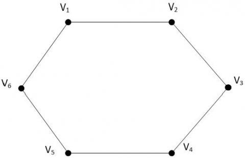
Example 3. Let us consider $\mathfrak{C}_6$ with $\mathfrak{B}\left(\mathfrak{C}_6\right)=$ $\left\{\mathfrak{v}_1, \mathfrak{v}_2, \ldots, \mathfrak{v}_6\right\}$ and $\mathfrak{E}\left(\mathfrak{C}_6\right)=\left\{\mathfrak{e}_1, \mathfrak{e}_2, \ldots, \mathfrak{e}_6\right\}$ shown in Figure 3. The degree-distance vector representation for $\mathfrak{C}_6$ w.r.t $\mathfrak{A}$ is given in Table 3. The resolving set for $\mathfrak{C}_6$ is $\left\{\mathfrak{v}_1, \mathfrak{v}_2\right\}$.
$\beta_\delta\left(\mathfrak{C}_n\right)=2$.
Table 3. Degree-distance vector $\mathfrak{C}_6$ w.r.t $\mathfrak{U}$
|
$\mathfrak{d}$ (…) |
$\mathfrak{v}_1$ |
$\mathfrak{v}_2$ |
$\mathfrak{v}_3$ |
$\mathfrak{v}_4$ |
$\mathfrak{v}_5$ |
$\mathfrak{v}_6$ |
|
$\mathfrak{A}=\left\{\mathfrak{v}_1, \mathfrak{v}_2 \right\}$ |
(0,4) |
(4,0) |
(8,4) |
(12,8) |
(8,12) |
(4,8) |
Figure 3. Rough cycle with 6 vertices C6
Theorem 3. The complete rough graph has a degree distance metric dimension of $\mathfrak{n}$-1.
Proof. The degree of each vertex will be same as the resolving number. The shortest distance between any two vertices will be 1. The vector representation of $\mathfrak{K}_n$ w.r.t $\mathfrak{A}$ will be:
$\mathfrak{r}\left(\mathfrak{v}_\alpha \mid \mathfrak{H}\right)=\left\{\begin{array}{cc}\left(0,(\delta(\mathrm{v}))^2, \ldots, \mathfrak{n}\left((\delta(\mathrm{v}))^2\right)\right), & \text { when } \alpha=1 \\ \left((\delta(\mathrm{v}))^2, 0, \ldots, \mathfrak{n}\left((\delta(\mathrm{v}))^2\right)\right), & \text { when } \alpha=2 \\ \cdot & \\ \cdot & \\ \cdot \\ \left((\delta(\mathrm{v}))^2,(\delta(\mathrm{v}))^2, \ldots(\mathfrak{n}-1)\left((\delta(\mathrm{v}))^2\right)\right), & \text { when } \alpha=\mathfrak{n}\end{array}\right.$
$\therefore \beta_\delta\left(\mathfrak{K}_{\mathfrak{n}}\right)=\mathfrak{n}-1$ for $\mathfrak{n}=3,4, \ldots$
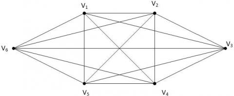
Example 4. Consider complete rough graph with 6 vertices and 15 edges as shown in Figure 4. The resolving set for Figure 4 is given Table 4.
Table 4. Degree-distance vector $\mathfrak{K}_6$ w.r.t $A$
|
$\mathfrak{d}$ (…) |
$\mathfrak{\mathfrak { U }}=\left\{\mathfrak{v}_1, \mathfrak{v}_2, \ldots, \mathfrak{v}_5\right\}$ |
|
$\mathfrak{v}_1$ |
(0,25,25,25,25) |
|
$\mathfrak{v}_2$ |
(25,0,25,25,25) |
|
$\mathfrak{v}_3$ |
(25,25,0,25,25) |
|
$\mathfrak{v}_4$ |
(25,25,25,0,25) |
|
$\mathfrak{v}_5$ |
(25,25,25,25,0) |
|
$\mathfrak{v}_6$ |
(25,25,25,25,25) |
Figure 4. Rough complete graph with 6 vertices
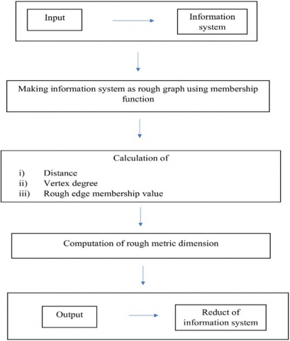
Figure 5. Flowchart to find reduct of an information system
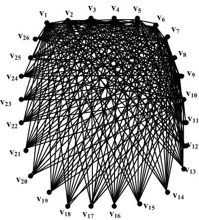
Figure 6. Rough graph
Figure 5 and Figure 6 represent the flow chart to find the reduct of an information system and the rough graph using information system respectively.
In this section, experimental findings are presented for an information system comprising 15 objects and 6 attributes, including a decision attribute. The investigation employs diverse degree-based distance formulas to identify the reduct within the information system.
Table 5. Decision system
|
|
$\mathbb{C}$ |
$\mathbb{BS}$ |
$\mathbb{CP}$ |
$\mathbb{F}$ |
$\mathbb{SB}$ |
$\mathbb{T}$ |
$\mathbb{FT}$ |
$\mathbb{A}$ |
$\mathbb{LD}$ |
$\mathbb{DM}$ |
$\mathbb{LC}$ |
|
$\wp_1$ |
1 |
1 |
1 |
0 |
1 |
1 |
1 |
1 |
1 |
0 |
2 |
|
$\wp_2$ |
1 |
1 |
1 |
0 |
1 |
1 |
1 |
1 |
1 |
0 |
2 |
|
$\wp_3$ |
1 |
1 |
1 |
0 |
1 |
1 |
1 |
1 |
1 |
0 |
2 |
|
$\wp_4$ |
1 |
1 |
1 |
0 |
1 |
1 |
1 |
1 |
1 |
0 |
2 |
|
$\wp_5$ |
1 |
1 |
1 |
0 |
1 |
1 |
1 |
1 |
1 |
0 |
2 |
|
$\wp_6$ |
1 |
1 |
1 |
0 |
1 |
1 |
1 |
1 |
1 |
0 |
2 |
|
$\wp_7$ |
1 |
1 |
1 |
0 |
1 |
1 |
1 |
1 |
1 |
0 |
2 |
|
$\wp_8$ |
1 |
1 |
1 |
0 |
1 |
1 |
1 |
1 |
1 |
0 |
2 |
|
$\wp_9$ |
1 |
1 |
1 |
1 |
1 |
1 |
1 |
1 |
1 |
1 |
2 |
|
$\wp_{10}$ |
1 |
1 |
1 |
0 |
1 |
1 |
1 |
1 |
0 |
1 |
2 |
|
$\wp_{11}$ |
1 |
1 |
1 |
0 |
1 |
1 |
1 |
1 |
0 |
1 |
3 |
|
$\wp_{12}$ |
1 |
1 |
1 |
0 |
1 |
1 |
1 |
1 |
0 |
1 |
3 |
|
$\wp_{13}$ |
1 |
1 |
1 |
0 |
1 |
1 |
1 |
1 |
0 |
1 |
3 |
|
$\wp_{14}$ |
1 |
1 |
1 |
0 |
1 |
1 |
1 |
1 |
0 |
1 |
3 |
|
$\wp_{15}$ |
1 |
1 |
1 |
0 |
1 |
1 |
1 |
1 |
0 |
1 |
3 |
|
$\wp_{16}$ |
1 |
1 |
1 |
0 |
1 |
1 |
1 |
1 |
0 |
1 |
3 |
|
$\wp_{17}$ |
1 |
1 |
1 |
1 |
1 |
0 |
0 |
0 |
0 |
1 |
3 |
|
$\wp_{18}$ |
1 |
0 |
1 |
0 |
1 |
0 |
0 |
0 |
0 |
0 |
3 |
|
$\wp_{19}$ |
1 |
0 |
1 |
0 |
1 |
0 |
0 |
0 |
0 |
0 |
4 |
|
$\wp_{20}$ |
1 |
0 |
1 |
0 |
1 |
0 |
0 |
0 |
1 |
0 |
4 |
|
$\wp_{21}$ |
1 |
0 |
1 |
0 |
1 |
0 |
0 |
0 |
1 |
0 |
4 |
|
$\wp_{22}$ |
1 |
0 |
1 |
0 |
1 |
0 |
0 |
0 |
1 |
0 |
4 |
|
$\wp_{23}$ |
1 |
0 |
1 |
0 |
1 |
0 |
0 |
0 |
1 |
0 |
4 |
|
$\wp_{24}$ |
1 |
0 |
1 |
0 |
1 |
0 |
0 |
0 |
1 |
0 |
4 |
|
$\wp_{25}$ |
1 |
0 |
1 |
0 |
1 |
0 |
0 |
0 |
1 |
0 |
4 |
|
$\wp_{26}$ |
1 |
0 |
0 |
0 |
1 |
0 |
0 |
0 |
0 |
0 |
4 |
The provided information system in Table 5 , denoted as $\mathfrak{J}=(\mathfrak{U}, \mathbb{D})$, involves a universe set $\mathfrak{U}=\left\{\mathfrak{v}_1, \mathfrak{v}_2, \ldots, \mathfrak{v}_{26}\right\}$ and is derived from a pool of 26 lung cancer patients. The information system encompasses both condition and decision attributes, denoted as $\mathbb{D}=\mathfrak{C} \cup \mathfrak{D}$, where $\mathfrak{C}$ represents the condition attributes and $\mathfrak{D}$ signifies the decision attribute. The condition attributes, namely cough, bloody sputum, chest pain, fever, shout breath, thin, feeling tired, anorexia, local diffusion and distant metastasis along with the three decision attributes, lung cancer, collectively form the elements of $\mathfrak{D}$. In this context, the binary values 0 and 1 correspond to no and yes, respectively, then 2, 3 and 4 correspond to central lung cancer, peripheral lung cancer and thin bronchuses lung bubble cancer respectively. This information system captures essential characteristics of lung cancer, utilizing the specified attributes to distinguish and analyze various aspects, ultimately contributing to a comprehensive understanding of the underlying data.
The rough membership function for the above information system is:
$\begin{gathered}\mu_{\mathfrak{X}}^{\mathfrak{B}}\left(\mathfrak{p}_1\right)=\frac{8}{10}, \mu_{\mathfrak{X}}^{\mathfrak{B}}\left(\mathfrak{p}_{14}\right)=0, \mu_{\mathfrak{X}}^{\mathfrak{B}}\left(\mathfrak{p}_2\right)=\frac{8}{10}, \mu_{\mathfrak{X}}^{\mathfrak{B}}\left(\mathfrak{p}_{15}\right)=0 \\ \mu_{\mathfrak{X}}^{\mathfrak{B}}\left(\mathfrak{p}_3\right)=\frac{8}{10}, \mu_{\mathfrak{X}}^{\mathfrak{B}}\left(\mathfrak{p}_{16}\right)=0, \mu_{\mathfrak{X}}^{\mathfrak{B}}\left(\mathfrak{p}_4\right)=\frac{8}{10}, \mu_{\mathfrak{X}}^{\mathfrak{B}}\left(\mathfrak{p}_{17}\right)=0 \\ \mu_{\mathfrak{X}}^{\mathfrak{B}}\left(\mathfrak{p}_5\right)=\frac{8}{10}, \mu_{\mathfrak{X}}^{\mathfrak{B}}\left(\mathfrak{p}_{18}\right)=0, \mu_{\mathfrak{X}}^{\mathfrak{B}}\left(\mathfrak{p}_6\right)=\frac{8}{10}, \mu_{\mathfrak{X}}^{\mathfrak{B}}\left(\mathfrak{p}_{19}\right)=0 \\ \mu_{\mathfrak{X}}^{\mathfrak{B}}\left(\mathfrak{p}_7\right)=\frac{8}{10}, \mu_{\mathfrak{X}}^{\mathfrak{B}}\left(\mathfrak{p}_{20}\right)=0, \mu_{\mathfrak{X}}^{\mathfrak{B}}\left(\mathfrak{p}_8\right)=\frac{8}{10}, \mu_{\mathfrak{X}}^{\mathfrak{B}}\left(\mathfrak{p}_{21}\right)=0 \\ \mu_{\mathfrak{X}}^{\mathfrak{B}}\left(\mathfrak{p}_9\right)=1, \mu_{\mathfrak{X}}^{\mathfrak{B}}\left(\mathfrak{p}_{22}\right)=0, \mu_{\mathfrak{X}}^{\mathfrak{B}}\left(\mathfrak{p}_{10}\right)=\frac{1}{7}, \mu_{\mathfrak{X}}^{\mathfrak{B}}\left(\mathfrak{p}_{23}\right)=0 \\ \mu_{\mathfrak{X}}^{\mathfrak{B}}\left(\mathfrak{p}_{11}\right)=0, \mu_{\mathfrak{X}}^{\mathfrak{B}}\left(\mathfrak{p}_{24}\right)=0, \mu_{\mathfrak{X}}^{\mathfrak{B}}\left(\mathfrak{p}_{12}\right)=0 \\ \mu_{\mathfrak{X}}^{\mathfrak{B}}\left(\mathfrak{p}_{25}\right)=0, \mu_{\mathfrak{X}}^{\mathfrak{B}}\left(\mathfrak{p}_{13}\right)=0, \mu_{\mathfrak{X}}^{\mathfrak{B}}\left(\mathfrak{p}_{26}\right)=0\end{gathered}$
Ensuring the concise representation of an entire information system is imperative, leading to the fundamental concept of a reduct. A reduct, in essence, acts as a minimal representation of the complete information system, encapsulating the most pertinent variables. The incorporation of rough metric dimension further refines this process by providing a systematic approach to discern the reduct set through graphical representation. This methodology is instrumental in distilling the essential components of the information system. In our exploration, we have delved into various degree-based metric dimensions to discern and establish the reduct. This investigative process not only enhances our understanding of the information system's core elements but also sets the stage for potential algorithmic developments. The objective is to create algorithms capable of efficiently computing reducts within information systems, streamlining the representation of crucial information. Looking forward, our future investigations aim to extend beyond the current scope, delving deeper into theoretical research and conducting applied analyses, specifically focusing on rough graphs. This expansion is driven by the recognition of the intricate relationships within rough graphs and the potential applications that can be derived from a more nuanced understanding. By combining theoretical exploration with practical applications, we strive to contribute to the broader understanding and utilization of rough graphs in diverse fields, fostering advancements in both theoretical frameworks and real-world implementations.
[1] Pawlak, Z. (1998). Rough set theory and its applications to data analysis. Cybernetics & Systems, 29(7): 661-688. https://doi.org/10.1080/019697298125470
[2] Anitha, K. (2014). Rough set theory on topological spaces. In Rough Sets and Knowledge Technology: 9th International Conference, RSKT 2014, Shanghai, China, pp. 69-74. https://doi.org/10.1007/978-3-319-11740-9-7
[3] Kausar, N., Munir, M., Kousar, S., Gulistan, M., Anitha, K. (2020). Characterization of non-associative ordered semigroups by the properties of F-ideals. Fuzzy Information and Engineering, 12(4): 490-508. https://doi.org/10.1080/16168658.2021.1924513
[4] Munir, M., Kausar, N., Anitha, K., Mani, G. (2024). Exploring the algebraic and topological properties of semigroups through their prime m-bi ideals. Kragujevac Journal of Mathematics, 48(3): 407-421.
[5] Kausar, N., Munir, M., Anitha, K. (2020). Left regular ordered Ag-groupoids. Advanced Mathematical Models and Applications, 5(3): 307-312.
[6] Kalaivani, N., Anitha, K., Saravanakumar, D., Sundarakrishnan, S. (2017). On Ω−operations in soft topological spaces. Far East Journal of Mathematical Sciences,101(9): 2067-2077. http://doi.org/10.17654/MS 10109067
[7] Lukshmi, R.A., Geetha, P.V., Venkatesan, P. (2013). Rough set theory approach for attribute reduction. Indian Journal of Automation and Artificial Intelligence, 1(3): 70-80.
[8] Anitha, K. (2021). Predictive analysis of COVID-19 transmission: Mathematical modeling study. In Emerging Technologies for Battling COVID-19: Applications and Innovations, pp. 295-307. https://doi.org/10.1007/978-3-030-60039-6_15
[9] Anitha, K., Datta, D. (2022). Analysing high dimensional data using rough tolerance relation. In 2022 International Conference on Electrical, Computer, Communications and Mechatronics Engineering (ICECCME), Maldives, Maldives, pp. 1-5. https://doi.org/10.1109/ICECCME55909.2022.9988257
[10] Anitha, K. (2022). Scaling-up redundant features using fuzzy-rough data analysis techniques. Journal of Northeastern University, 24(4): 2642-2657.
[11] Anitha, K., Venkatesan, P. (2016). Properties of hesitant fuzzy sets. Global Journal of Pure and Applied Mathematics, 12(1): 114-116.
[12] Anitha, K., Datta, D. (2021). Fuzzy-rough optimization technique for breast cancer classification. In International Conference on Nonlinear Applied Analysis and Optimization, Varanasi, India, pp. 423-435. https://doi.org/10.1007/978-981-99-0597-3_30
[13] Anitha, K., Datta, D. (2023). Type-2 fuzzy set approach to image analysis. In Recent Trends on Type-2 Fuzzy Logic Systems: Theory, Methodology and Applications, pp. 187-200. https://doi.org/10.1007/ 978-3-031-26332-3-12
[14] Anitha, K., Thangeswari, M. (2020). Rough set based optimization techniques, 6th International Conference on Advanced Computing and Communication Systems (ICACCS), Coimbatore, India, pp. 1021-1024, https://doi.org/10.1109/ICACCS48705.2020.9074212
[15] Anitha, K. (2021). Social media data analysis: rough set theory based innovative approach. In Intelligence of Things: AI-IoT Based Critical-Applications and Innovations, pp. 209-226. https://doi.org/10.1007/978-3-030-82800-4_9
[16] He, T., Lu, C.J., Shi, K.Q. (2006). Rough graph and its structure. Journal of Shandong University, 41(6): 46-50.
[17] He, T., Chen, Y., Shi, K.Q. (2006). Weighted rough graph and its application. In Sixth International Conference on Intelligent Systems Design and Applications, Jinan, China, pp. 486-491. https://doi.org/10.1109/ISDA.2006.279
[18] Shu, L., He, X. (2007). Rough set model with double universe of discourse. In 2007 IEEE International Conference on Information Reuse and Integration, Las Vegas, NV, USA, pp: 492-495. https://doi.org/10.1109/IRI.2007.4296668
[19] He, T., Xue, P., Shi, K. (2008). Application of rough graph in relationship mining. Journal of System Engineering Electronics, 19(4): pp: 742-747. https://doi.org/10.1016/S1004-4132(08)60147-4
[20] Liang, M., Liang, B., Wei, L., Xu, X. (2011). Edge rough graph and its application. In 2011 Eighth International Conference on Fuzzy Systems and Knowledge Discovery (FSKD), Shanghai, China, pp. 335-338. https://doi.org/10.1109/FSKD.2011.6019588
[21] He, T. (2012). Rough properties of rough graph. Applied Mechanics and Materials, 157: 517-520. https://doi.org/10.4028/www.scientific.net/AMM.157-158.517
[22] He, T., Yang, R. (2017). Different kinds of rough graph and their representation forms. DES tech Transactions on Engineering and Technology Research. https://doi.org/10.12783/dtetr/mdm2016/4929
[23] Shah, N., Rehman, N., Shabir, M., Irfan Ali, M. (2018). Another approach to roughness of soft graphs with applications in decision making. Symmetry, 10(5): 145. https://doi.org/10.3390/sym10050145
[24] Mathew, B., John, S.J., Garg, H. (2020). Vertex rough graphs. Complex & Intelligent Systems, 6(2), 347-353. https://doi.org/10.1007/s40747-020-00133-8
[25] Akram, M., Arshad, M., Shumaiza. (2018). Fuzzy rough graph theory with applications. International Journal of Computational Intelligence Systems, 12(1): 90-107. https://doi.org/10.2991/ijcis.2018.25905184
[26] Akram, M., Zafar, F. (2019). Rough fuzzy graphs. In Studies in Fuzziness and Soft Computing, pp. 1-77. https://doi.org/10.1007/978-3-030-16020-3_1
[27] Aruna Devi, R., Anitha, K. (2022). Construction of rough graph to handle uncertain pattern from an information system. Mathematics and Statistics, 10(6): 1344-1353. https://doi.org/10.13189/ms.2022.100622
[28] Anitha, K., Aruna Devi, R., Munir, M., Nisar, K.S. (2021). Metric dimension of rough graphs. International Journal of Nonlinear Analysis and Applications, 12(1): 1793-1806. https://doi.org/10.22075/ijnaa.2021.5891
[29] Nithya, R., Anitha, K. (2023). Even vertex ζ−graceful labeling on rough graph. Mathematics and Statistics, 11(1): 71-77. https://doi.org/10.13189/ms.2023.110108
[30] Nithya, R., Anitha, K. (2022). Extensive types of graph labelling on rough approximations. Telematique, 21(1): 3251-3261.
[31] Nithya, R., Anitha, K. (2023). Rough set techniques in wireless sensor networks using membership function and rough labelling graphs for energy aware routing. International Journal on Recent and Innovation Trends in Computing and Communication, 11(9): 2545-2556.
[32] Wang, D., Zhu, P. (2022). Graph reduction in a path information-based rough directed graph model. Soft Computing, 26(9): 4171-4186. https://doi.org/10.1007/s00500-022-06887-2
[33] Majumder, S., Kar, S. (2018). Multi-criteria shortest path for rough graph. Journal of Ambient Intelligence and Humanized Computing, 9: 1835-1859, https://doi.org/10.1007/s12652-017-0601-6
[34] Akram, M., Arshad, M., Shumaiza. (2018). Fuzzy rough graph theory with applications. International Journal of Computational Intelligence Systems, 12(1): 90-107. https://doi.org/10.2991/ijcis.2018.25905184
[35] He, T., Xue, P., Shi, K. (2008). Application of rough graph in relationship mining. Journal of Systems Engineering and Electronics, 19(4): 742-747. https://doi.org/10.1016/S1004-4132(08)60147-4
[36] Rebenciuc, M., Bibic, S.M. (2017). Generalized rough sets applied to graphs related to urban problems. International Journal of Mathematical and Computational Sciences, 11(9): 411-416.
[37] Ahmad, U., Nawaz, I. (2022). Directed rough fuzzy graph with application to trade networking. Computational and Applied Mathematics, 41(8): 366. https://doi.org/10.1007/s40314-022-02073-0