Eka Mala Sari Rochman*![]() | Wahyudi Setiawan
| Wahyudi Setiawan![]() | Shofia Hardi
| Shofia Hardi![]() | Kurniawan Eka Permana
| Kurniawan Eka Permana![]() | Husni
| Husni![]() | Yuli Panca Asmara
| Yuli Panca Asmara![]() | Aeri Rachmad
| Aeri Rachmad![]()
© 2024 The authors. This article is published by IIETA and is licensed under the CC BY 4.0 license (http://creativecommons.org/licenses/by/4.0/).
OPEN ACCESS
Salt is one of the commodities in Indonesia. Salt has a very strategic and sustainable role for human life. Apart from being used for daily consumption, salt is also used as a raw material for various industries Indonesia, as a country surrounded by coastlines, can be self-sufficient in salt production and meet domestic salt needs. However, not all the salt produced maintains sufficient quality for consumption. Therefore, monitoring of the produced salt's quality is necessary to categorize it. Even though the categorization of salt quality is still carried out manually, this research employs data mining techniques with three different algorithms: Naïve Bayes, K-Nearest Neighbor (K-NN), and Support Vector Machine (SVM), to simplify and enhance the efficiency of the classification process. The dataset used was obtained from salt data in the Sumenep region of Madura that consists of 349 records with seven attributes: sulfate, magnesium, water content, calcium, not dissolved, NaCl(wb), and NaCl(db) with four data classes that represent grades of salt quality (K1, K2, K3, and K4), and the salt data is divided into training and testing sets using the k-fold cross-validation method. Test results indicate that the K-NN method provides better outcomes compared to other methods, with an AUC value reaching 99.0%, accuracy of 91.7%, F1 Score reaching 91.6%, precision of around 91.9%, and recall of around 91.7%.
salt quality, consumption, classification, support vector machine, naïve Bayes, K-Nearest Neighbor
As one of the largest commodities in Indonesia, salt plays a crucial and essential role for humans, both in the form of table salt for consumption and as a raw material in various industries [1-3]. In Indonesia, salt can be categorized into two main types: consumption salt and industrial salt [4, 5]. Consumption of salt is used in food and plays a vital role in maintaining electrolyte balance in the human body. On the other hand, industrial salt is utilized across various sectors, including the chemical, pharmaceutical, textile industries, and more. Therefore, the quality of salt is of utmost importance, both for human health and for maintaining the quality of industrial products [6].
The challenge regarding salt quality in Indonesia is still an interesting matter, even though Indonesia has significant salt production potential. Not all salt produced meets the necessary standards for consumption or use in industries. Factors such as contamination, mineral content, and concentrations of active compounds play a role in determining salt quality [7]. Therefore, monitoring and testing the quality of salt are essential tasks. The mineral form of halite, or rock salt, is sometimes called common salt (NaCl) to distinguish it from a class of chemical compounds called salts. Salt, usually called rock salt (Mineral halite), is used to distinguish between chemical compounds called salts. In contrast to the world salt classification, the national salt classification is broadly grouped into two types of salt, namely consumption salt and industrial salt.
In enhancing the monitoring and control of salt quality, technologies like data mining and statistical analysis are highly valuable [8]. These methods assist in categorizing salt based on its quality, which in turn helps identify salt that meets standards and can be used safely. Research involving the use of data mining techniques to classify salt quality, as mentioned earlier, represents a progressive step in optimizing salt production and usage in Indonesia. Similar to a study conducted in 2019 regarding classification using the C4.5 method, the proposed method in this research is not yet able to classify optimally due to its inability to handle datasets with a large number of classes [9]. The variety of machine learning methods that can be used in the data mining process has led several researchers to study several methods in one case study to compare the results of the algorithm's performance, such as in research in 2019. This research compared two different methods, namely Naïve Bayes and C4 .5. Based on the results obtained, the Naïve Bayes method is superior to C4.5 in classifying a dataset. Meanwhile, in research comparing three methods for classifying numerical data, the SVM and KNN methods had more optimal accuracy results compared to the Decision Tree method where the SVM algorithm had the best accuracy in predictions with an accuracy value of 95% [10, 11].
Based on previous research, the researchers were intrigued to examine the implementation of various different algorithms to construct a classification system for salt quality. The data used in this study consists of salt data obtained from the Sumenep Regency, which is the largest salt-producing region on Madura Island [12].
Overall, understanding the importance of salt and its quality in Indonesia plays a crucial role in maintaining human health and supporting various industrial sectors. With research and development efforts as described above, it is hoped that salt management in Indonesia will be further improved, both in terms of sustainable production and in terms of meeting higher quality standards. Therefore, this research proposes the KNN classification method to obtain the most optimal classification modeling system in categorizing salt quality which will be compared with several classification methods including Support Vector Machine and Naïve Bayes.
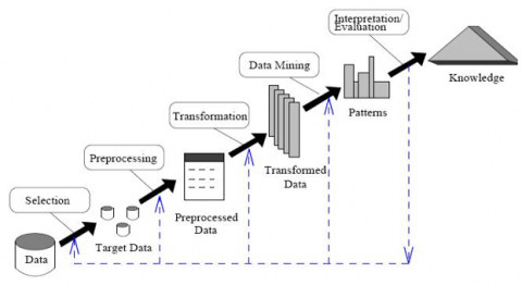
This study discusses the classification of salt quality using numerical data. Classification is one of the scientific disciplines in data mining which involves the process of extracting, identifying, and analyzing various information with the aim of discovering patterns within data using mathematical, statistical, artificial intelligence, and machine learning approaches [13, 14]. Data mining is known as the discovery of knowledge in databases. several types of data mining based on their function, including description, prediction, estimation, classification, clustering, and association [15]. Figure 1 shows the steps in data mining.
Figure 1. Data mining
Here is an explanation of the steps in the data mining process:
(1) Data Selection: remove irrelevant and inconsistent data.
(2) Data Cleaning: Involves merging and adding data that is relevant.
(3) Data Select: This involves choosing data to be used as the basis for analysis.
(4) Data Transformation: Before the mining process, the data is converted into a certain format.
(5) Data Mining: Involves searching for information using data mining methods.
(6) Evaluation: Involves identifying patterns from data obtained by the method and then evaluating the results and the hypothesis.
2.1 Data
The quality of salt is categorized into several classes based on its intended use. In all cases, it is important to understand the purpose of using salt and ensure that the salt used meets the required standards to maintain human health and product quality. In categorizing salt into classes K1, K2, K3, and K4, there are several features used in this study, which will be explained as follows:
(1) Water Content
Water content is one of the features used in this study to classify the quality of salt. This feature is employed because the moisture content in salt significantly impacts its quality. If the moisture content in salt is too high, the salt's durability will decrease [16].
(2) Not Dissolved
Salt is a compound made up of sodium, and almost all of it is soluble in water, including salt itself. Because of this feature, it is necessary to use it for classifying the quality of salt, as higher-quality salt tends to have a higher solubility level. Salt that readily dissolves is highly recommended for consumption as it is beneficial for health [17].
(3) Calcium
Calcium is one of the elements present in salt, thus the concentration of calcium also affects the quality of salt [18]. Salt that is suitable for consumption should have a maximum calcium content of 0.06% [17].
(4) Magnesium
Magnesium is also one of the elements present in salt, so the concentration of magnesium affects the quality of salt [18]. Salt that is suitable for consumption should have a maximum magnesium content of 0.06% [17].
(5) Sulfate
Sulfate is a compound that can decrease the NaCl content in salt, whereas good quality salt should have a minimum NaCl content of 97%. Therefore, if the sulfate content is detected to be high, it can degrade or lower the quality classification of the salt [17].
(6) NaCl (wb) and (db)
In this study, the features used are NaCl wet basis and dry basis to categorize salt data into classes based on their quality. Salt that meets the food grade standard must have a minimum NaCl content of 97% [17].
2.2 Data pre-processing
Data preprocessing is the initial step before entering the model training phase, aimed at organizing the input dataset into a structured format to facilitate the training process [19]. In this study, the data preprocessing stage involves data transformation to adapt the data format according to the requirements.
2.2.1 Data transformation
Data transformation involves modifying the scale of data into a different format to achieve the desired data distribution. Each data point undergoes similar mathematical operations as its original form [20]. One method of data transformation is data normalization, which aims to adjust several variables to have a uniform range of values to prevent overly large or small values that might affect analysis outcomes. The primary objective of altering all data is to maintain the relative differences between data points. If multiple variables are present, the transformation is applied to all variables to preserve the relationships between data points [21]. The process of data normalization is implemented using the Min-Max normalization technique, defined by Eq. (1) below:
$z=\frac{x-\min (x)}{\lceil\max (x)-\min (x)\rceil}$ (1)
where, z: normalization result, x: x value, min(x): minimal value of x, max(x): maximal value of x.
2.3 Data mining
Within this research, the data mining procedure includes dividing the data into training and testing datasets. The training dataset is used to train the model, whereas the testing dataset is employed for validation and assessment to gauge the effectiveness of the utilized techniques. The separation of the dataset is achieved through the implementation of the K-Fold Cross Validation approach, where the parameter "k" determines the dataset divisions. For instance, when using 5-Fold validation, the dataset is divided into four subsets for training and one subset for testing, with nearly equal sample sizes in each fold [22]. Subsequently, the classification process employs three different algorithms to construct a classification model capable of categorizing the quality of salt. These algorithms include K-Nearest Neighbor (KNN), Support Vector Machine and Naïve Bayes.
The advantage of the KNN method is that apart from being easy to implement and adapt, this method has few hyperparameters. For SVM, the advantage is that this method has two free parameters called upper bound and kernel parameters. SVM also produces unique and optimal solutions, and can implement the principle of structural risk minimization (SRM) which is known to have good general performance. Meanwhile, Naive Bayes has the advantage that this method is simple, fast and has high accuracy.
2.3.1 K-Nearest Neighbor (KNN)
K-Nearest Neighbor is an example of instance-based learning and is often used for classification tasks, where its objective is to classify unseen data based on the stored database. The new data point is classified based on its similarity to other data points stored in the model using various similarity metrics. The algorithm determines the class of the new point by selecting the K nearest points, also known as K neighbors, to the new data and choosing the most common class among the group of data points through majority vote as the class of the new point [23]. Several steps required for the implementation of this method can be outlined as follows:
(1) k values that have nearest neighbors must be determined at the beginning.
(2) Calculate the squared distance between the object point and the training data. In this study, the distance between object points is calculated using the Euclidean Distance method. Euclidean distance is a method of searching between two variable points, the closer and similar they are, the smaller the distance between the two points. Which is formulated in the Eq. (2):
$\operatorname{dist}(x, y)=\sqrt{\sum_{i=1}^n(X i-Y i)^2}$ (2)
where, d(x, y): Euclidian distance, X: Data 1, Y: Data 2, i: Attribute I, n: Number of attributes.
(1) After that, the results from the second step are sorted from the highest value to the lowest.
(2) Collect categories from the neighboring data based on the value of k.
(3) The final step, determines the majority category of nearest neighbors to be used to predict new data objects.
The K-NN method is often used for classifying data due to its simple and straightforward implementation, quick training process, and its applicability to data with noise. However, this method also has its drawbacks. It falls under the category of lazy algorithms, which can lead to slightly longer program execution times. It is highly sensitive when dealing with cases involving irrelevant features and requires memory storage for storing the training data records used in the process.
2.3.2 Naïve Bayes
Naïve Bayes is a simple probabilistic classification method that calculates various probability ranges by summing occurrences and combined values from the provided dataset. This algorithm employs Bayes’ theorem and assumes that all attributes are independent or non-interdependent based on the value of the class variable. An alternative description states that Naïve Bayes is a classification method that utilizes probability techniques and statistical insights developed by the British scientist, Thomas Bayes. It predicts future prospects using previous experiences as a reference foundation [10, 24].
This algorithm is a probability technique used to categorize classes in a given dataset. The basic outline of the Naïve Bayes method involves statistical analysis where initial probabilities (prior probabilities) are estimated from training data. The probabilities for each parameter are then calculated based on these initial probabilities. Its main characteristic is the strong assumption of the independence of certain phenomena or conditions. In the context of Bayes' theorem, when there are two distinct events, denoted as X and Y, Bayes' theorem can be expressed through Eq. (3) [24]:
$P(Z \mid Y)=\frac{P(Z)}{P(Y)} P(Y \mid Z)$ (3)
where, Z: New data record, Y: Hypothesis, P(Y|Z): Probability of Y toward Z hypothesis, P(Y): Probability hypothesis Y, P(Z|Y): Probability of Z based on the condition of Y, P(Z): Probability of Z.
The selection of this method is relatively straightforward as it doesn't involve matrix multiplication or numerical optimization. This method is more efficient when used for predicting large amounts of data and provides a relatively high level of accuracy in its prediction outcomes. However, this method cannot be applied to case studies that involve conditional probabilities with a value of zero, as the predicted probabilities will also be zero.
2.3.3 Support vector machine
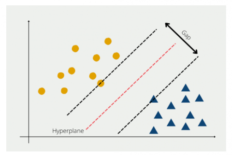
The method of Support Vector Machine (SVM), introduced by Boser, Guyon, and Vapnik in 1992 at the Annual Workshop on Computational Learning Theory, serves as a machine learning technique applicable for both classification and prediction purposes. SVM's core concept in classification involves identifying an optimal separator, known as a hyperplane. The hyperplane is deemed optimal when it offers the largest margin, representing twice the distance between the hyperplane and support vectors. These vectors refer to the nearest data points to the hyperplane. SVM excels in managing high-dimensional data and limited training samples due to its adherence to the Structural Risk Minimization (SRM) principle, which maximizes margin and minimizes expected risk in the face of uncertainty [25].
Figure 2. Support vector machine
Figure 2 illustrates 2 classes, each marked with distinct patterns. In Figure 2, the two classes are isolated by a ran red line known as the hyperplane. In this algorithm, the hyperplane is changed in accordance with be ideal for isolating the two distinct classes. The best optimal the resulting hyperplane is, the lower the error rate can be in the classification system.
In addition to handling linear data issues, SVM is also capable of addressing problems with data that cannot be linearly separated, also known as non-linear data. Non-linear problems can be overcome by utilizing kernels in a higher-dimensional workspace [26, 27]. There are various variations within the SVM method, including:
(1) Kernel Linier
Linear kernel functions are used for linear data classification. Linear kernel is the simplest kernel function. Linear kernels are used when the data being analysed is linearly separated.
$K\left(x_i, x\right)=x_i^T x$ (4)
(2) Kernel Polynomial
The polynomial kernel function is a kernel function that is used when the data is not linearly separated.
Polynomial kernels are a more general form of linear kernels. In machine learning, a polynomial kernel is a kernel function suitable for use in SVMs and other kernelizations, where the kernel represents the similarity of training sample vectors in feature space. Polynomial kernels are also suitable for solving classification problems on normalized training datasets.
$K\left(x_i, x\right)=\left(\gamma x_i^T+r\right)^p, \gamma>0$ (5)
(3) Kernel Radial Basis Function
The Radial Basis Function (RBF) kernel function is used for non-linear data classification. The RBF kernel or also called the Gaussian kernel is the kernel concept that is most widely used to solve data classification problems that cannot be separated linearly. This kernel is known to have good performance with certain parameters, and the results of training have a small error value compared to other kernels.
$K\left(x_i, x\right)=\exp \left(-\gamma\left\|x-x_i\right\|^2\right)$ (6)
(4) Sigmoid Kernel
$K\left(x_i, x\right)=\tanh \left(\gamma x_i^T+\mathrm{r}\right)$ (7)
The following are the steps in carrying out classification using the SVM method, among others:
(1) The initial stage involves computing the Hessian matrix, which results from the multiplication of the kernel function by the values of $y$. The value of $y$ corresponds to the vector value, namely the values 1 and -1 . Calculation of the Hessian matrix using Eq. (8).
$D_{i j}=y_{i,} y_j\left(K\left(x_i, x_j\right)+\lambda^2\right)$ (8)
where,
ij: The component of the Hessian matrix (i is row and j is column).
λ: The theoretical limits that will be derived.
yI: The class of i data.
yj: The class of j data.
(2) Next, the second phase entails evaluating the error value utilizing Eq. (9), computing delta alpha through Eq. (10), and ascertaining the updated alpha using Eq. (11), outlined in the subsequent manner.
$E_i=\sum_{i=1}^l a_i D_{i j}$ (9)
$\delta a_i=\min \left\{\max \left[\gamma\left(1-E_I\right),-a_i\right), C-a_i\right\}$ (10)
$a_i=a_i \delta a_i$ (11)
where,
$E_I$: error score
$a_i$: alpha
$\delta a_i$: delta alpha
C: Constanta
$b=-\frac{1}{2}\left(w \cdot x^{+}+w \cdot x^{-}\right)$ (12)
(4) The step four, calculating the dot product on training and testing data.
(5) The final step is to determine the class of the test data using the equation below:
$f(x)=\sum_{i=1}^l a_i y_i K\left(x_i, x\right)+b$ (13)
The SVM method is often used for in classifying data in previous studies, mainly due to its excellent accuracy and relatively easy training process. This method also adapts well to high-dimensional datasets. The balance between model complexity and error can be managed easily, and it can handle both continuous and categorical data. However, a notable drawback of this method is its difficulty in interpretation unless the features are easily understandable. Additionally, there's a lack of result transparency due to its non-parametric methodology.
2.4 Evaluation
To measure the accuracy level and performance outcomes of the algorithm, various methods can be employed. In this research, the Confusion Matrix method was used as a process for evaluation. Confusion Matrix is an evaluation method which calculates precision, accuracy, recall and F-measure of algorithm predictions based on test data [28]. Table 1 is a Confusion Matrix used as a reference for calculating accuracy, precision, recall, F1 Score and AUC values.
Table 1. Confusion matrix
|
|
Predicted |
||
|
Positive |
Negative |
||
|
Actual |
Positive |
TP |
FP |
|
Negative |
FN |
TN |
|
Based on the confusion matrix Table 1, the values of accuracy, precision, recall, F1 Score, and AUC can be calculated using the equations below:
(1) Accuracy
Accuracy $=\frac{T P+T N}{T P+T N+F P+F N}$ (14)
(2) Precision
Precision $=\frac{T P}{T P+E P} \times 100 \%$ (15)
(3) Recall
Recall $=\frac{T N}{T N+F N} \times 100 \%$ (16)
(4) F1 Score
$F-$ measure $=2 \times \frac{\text { Recall } x \text { Precision }}{\text { Recall }+ \text { Precision }} \times 100 \%$ (17)
(5) AUC
$A U C=\frac{1}{2} x\left(\frac{T P}{T P+F N}+\frac{T N}{T N+F P}\right)$ (18)
where, TP: Total number of true positive predictions, TN: Total number of data instances with actual positive class but predicted as negative, FN: Total number of true negative predictions, FP: Total number of data instances with actual negative class but predicted as positive.
3.1 Data gathering
Salt quality data was taken from salt pond water in the Sumenep district, consisting of 349 records and 7 attributes: sulfate, magnesium, water content, calcium, not dissolved, NaCl(wb), and NaCl(db). The class in the data represents the grade of salt quality, categorized into 4 classes K1 – K4. Table 2 shows the dataset used in this study.
Table 2. Dataset
|
Data |
Water content |
Not dissolved |
Calcium |
Magnesium |
Sulfate |
NaCl (wb) |
NaCl (db) |
Grade |
|
1 |
7,8278 |
0,0423 |
0,2403 |
0,8073 |
1,3472 |
83,9156 |
91,0422 |
K1 |
|
2 |
8,1081 |
0,5904 |
0,2169 |
0,9543 |
1,1831 |
85,012 |
92,513 |
K1 |
|
3 |
8,7838 |
0,0293 |
0,2008 |
0,9503 |
1,1129 |
84,3214 |
92,4413 |
K1 |
|
4 |
5,8712 |
0,2119 |
0,5413 |
0,9038 |
1,1152 |
88,182 |
93,6823 |
K2 |
|
5 |
4,6614 |
0,1755 |
0,4187 |
0,5303 |
1,4787 |
89,2901 |
93,6585 |
K2 |
|
6 |
8,4905 |
0,1812 |
0,2413 |
0,8135 |
1,2768 |
85,0348 |
92,9246 |
K2 |
|
7 |
8,7452 |
0,2021 |
0,3119 |
0,4813 |
1,2279 |
84,4195 |
92,5097 |
K2 |
|
8 |
11,2674 |
0,1987 |
0,3403 |
0,8849 |
1,0247 |
80,2015 |
90,4875 |
K3 |
|
9 |
7,6923 |
0,6548 |
0,4319 |
0,7775 |
1,4162 |
84,2949 |
91,3195 |
K3 |
|
10 |
8,0305 |
0,2969 |
0,2210 |
0,4112 |
0,9332 |
88,264 |
95,9711 |
K4 |
3.2 System architecture
In this section, we will elaborate on how the research is conducted using the previously described methods, as an effort to address the raised issues. The following are the steps in the classification process that will be represented through an IPO diagram presented below.
Figure 3. IPO diagram
Based on Figure 3, the classification stages are divided into three stages, namely, process input and output. The explanations for each of these three stage components are as follows:
(1) Data Input Process
This process marks the initial stage of data mining by inputting the dataset to be classified, where the dataset used consists of 7 salt-related features.
(2) Preprocessing
Data transformation is carried out in this process, namely normalizing the data using a min max scaler so that the data used has a range of values that are not much different, namely ranging from 0 to 1.
(3) Splitting Process
Dividing training and testing data using k-fold cross validation with k values of 5, 10 and 20. The training data is essential for building the classification model, utilizing a certain portion of the overall data. The testing data, on the other hand, remains unused during the training phase and is used to validate the model's performance.
(4) Classification
In this process, learning is carried out to get the best classification model using machine learning methods including KNN, Support Vector Machine and Naïve Bayes. The training results provide knowledge about the model in classifying data. Testing on both training data and test data was carried out to find out what level of salt quality is good. By comparing different classification models, this is done in order to get a comparison of which method is appropriate and accurate in classifying optimally.
(5) Output
The output results from this classification process will categorize the attribute data on salt into classes based on the modelling that has been carried out. The salt quality level resulting from the classification of each algorithm is analysed and evaluated using the Confusion Matrix.
4.1 K-Nearest Neighbor (K-NN)
At this stage the salt dataset is classified using the KNN method with k=5. In this classification process, 3 scenario trials are used, namely on folds 5, 10 and 20. The results obtained from the application of this method can be seen in the following Table 3.
Table 3. Evaluation result of K-NN
|
Fold |
AUC |
Classification Accuracy |
F1 Score |
Precision |
Recall |
|
5 |
98.7% |
90.3% |
89.9% |
90.6% |
90.3% |
|
10 |
99.0% |
91.7% |
91.6% |
91.9% |
91.7% |
|
20 |
99.0% |
90.3% |
90.1% |
90.2% |
90.3% |
In Table 3, it is shown that the AUC value is highest at k=10 and k=20, with a value of 99.0%. Furthermore, the best evaluation in general results were obtained when k=10, with an accuracy of 91.7%, an F1 Score of 91.6%, precision of 91.9%, and recall of 91.7%.
4.2 Support vector machine
By applying the Support Vector Machine method to classify salt quality, good results were obtained as seen in Table 4. These evaluation results were achieved when using the parameters indicated in Table 4 and involving dataset splitting through k-fold values, namely 5, 10, and 20.
Table 4. Parameter SVM
|
Kernel |
RBF (Radial Basis Function) |
|
Coefficient Kernel |
Scale $\left(1 /\left(n \_\right.\right.$features $\left.\left.* X . \operatorname{var}()\right)\right)$ |
|
Cost Value (C) |
1.00 |
|
Epsilon |
0.10 |
|
Iteration |
100 |
Table 5. Evaluation result of SVM
|
Fold |
AUC |
Classification Accuracy |
F1 Score |
Precision |
Recall |
|
5 |
87.7% |
70.3% |
69.8% |
71.4% |
70.3% |
|
10 |
88.2% |
70.9% |
70.4% |
72.0% |
70.9% |
|
20 |
87.7% |
71.7% |
71.2% |
72.6% |
71.7% |
From the three tests with varying k-fold values, the best performance was achieved when k=20. While the highest AUC value was observed at k=10, the classification accuracy, F1 Score, precision, and recall were better when k=20, as shown in Table 5. Specifically, this configuration resulted in an AUC value of 87.7%, an accuracy of 71.7%, an F1 Score of 71.2%, a precision of 72.6%, and a recall of 71.7%.
4.3 Naïve Bayes
The results obtained in this study, using the salt dataset and the Naïve Bayes algorithm, involved dataset division through k-folds values, namely 5, 10, and 20.
Among the three tests with different k-fold values, the best performance was achieved when k=10, as indicated in Table 6. This resulted in an AUC value of 78.55%, an accuracy of 55.7%, an F1 Score of 56.0%, a precision of 56.9%, and a recall of 55.7%.
Table 6. Evaluation result of Naive Bayes
|
Fold |
AUC |
Classification Accuracy |
F1 Score |
Precision |
Recall |
|
5 |
77.7% |
54.9% |
54.9% |
55.8% |
54.9% |
|
10 |
78.5% |
55.7% |
56.0% |
56.9% |
55.7% |
|
20 |
77.7% |
54.9% |
55.1% |
56.1% |
54.9% |
The results of the tests that have been carried out are comparing the three methods, which one is more accurate. The comparison of the performance of each algorithm model can be seen in Table 7.
Table 7. Comparison evaluation results of AUC values for the KNN, SVM and Naïve Bayes methods with fold 10
|
Method |
AUC |
Accuracy |
|
K-NN |
99.0% |
91.7% |
|
SVM |
88.2% |
70.9% |
|
Naïve Bayes |
78.5% |
55.7% |
It can be seen that the KNN algorithm is superior to the SVM and Naïve Bayes algorithms for multivariate data types with an accuracy value of 96%. The K-NN method is very good in predictions, but when used on the multivariate data type in this study. This shows that the classification and prediction algorithm models are getting better too. Based on the results of the accuracy, precision, recall and F1-Score values, it can be concluded that the KNN algorithm has better performance than the SVM and Naive Bayes algorithms in classifying salt quality.
System identification allows all classification classes, and feature engineering plays an important role in increasing the accuracy of classification models. The opportunities and challenges of machine learning have been explored in this research. This shows that salt data is a source of data for classification. However, in order for this potential to be realized, it is necessary to develop methods that are effective and able to handle these conditions.
Based on the analysis and discussion conducted on the training and testing data using different k-fold values on a dataset containing 349 records and 7 attributes such as sulfate, magnesium, water content, calcium, not dissolved, NaCl(wb), and NaCl(db), the following conclusions can be drawn:
(1) Based on Tables 3-6 in testing the comparison of k-fold values in the three methods, the k-fold value=10 gets the best evaluation results compared to 5 and 20 when applying the KNN, SVM and Naïve Bayes methods.
(2) Of the three classification methods used in this research, KNN provides the best accuracy values with AUC values reaching 99.0%, accuracy is 91.7%, F1 Score is 91.6%, precision is 91.9% and recall is 91.7%. This is because KNN is robust against noise data. And it is a well-known classification algorithm with a good level of accuracy. The advantage of the KNN algorithm is that it is very nonlinear, easier to understand and implement because it defines a function to calculate the distance between instances.
The suggestions for further development and research are:
(1) For future studies, it is recommended to consider adding more features that can be used as criteria for categorizing salt into its quality classes.
(2) There is a need for the development of a system using deep learning methods to achieve more optimal classification model results.
The researcher would like to thank University of Trunojoyo Madura, especially the University's Research and Community Service Institute for supporting the research, as well as to the Faculty of Engineering which is the researchers' home base.
[1] Kustiyahningsih, Y., Rahmanita, E., Rachmad, A., Purnama, J. (2021). Integration interval type-2 FAHP-FTOPSIS group decision-making problems for salt farmer recommendation. Communications in Mathematical Biology and Neuroscience, 2021: 92. https://doi.org/10.28919/cmbn/6930
[2] Fuad, M., Rochman, E.M.S., Rachmad, A. (2022). Salt Commodity data clustering using fuzzy C-means. Journal of Physics: Conference Series, 2406(1): 012025. https://doi.org/10.1088/1742-6596/2406/1/012025
[3] Abdullah, A., Shalihati, F. (2020). The effectiveness of the salt policy in Indonesia. Jurnal Manajemen & Agribisnis, 17(3): 315-315. http://doi.org/10.17358/jma.17.3.315
[4] Tebay, V. (2023). Indonesian policy choices on salt. Formosa Journal of Applied Sciences, 2(7): 1601-1610. https://doi.org/10.55927/fjas.v2i7.5005
[5] Rochman, E.M.S., Rachmad, A., Fatah, D.A., Setiawan, W., Kustiyahningsih, Y. (2022). Classification of salt quality based on salt-forming composition using random forest. Journal of Physics: Conference Series, 2406(1): 012021. https://doi.org/10.1088/1742-6596/2406/1/012021
[6] Khozaimi, A., Pramudita, Y.D., Rochman, E.M.S., Rachmad, A. (2019). Salt quality determination using simple additive weighting (SAW) and analytical hirarki process (AHP) methods. Jurnal Ilmiah Kursor, 10(2): 227. https://doi.org/10.21107/kursor.v10i2.227
[7] Khozaimi, A., Pramudita, Y.D., Rochman, E.M.S., Rachmad, A. (2020). Decision support system for determining the quality of salt in Sumenep Madura-Indonesia. Journal of Physics: Conference Series, 1477(5): 052057. https://doi.org/10.1088/1742-6596/1477/5/052057
[8] Chang, Q., Hu, J. (2022). Research and application of the data mining technology in economic intelligence system. Computational Intelligence and Neuroscience, 2022: 6439315. https://doi.org/10.1155/2022/6439315
[9] Abdillah, N., Ihksan, M. (2022). Application of the C4. 5 algorithm for classification of medical record data at M. Djamil Hospital based on the international disease code. Jurnal Mantik, 6(1): 576-581. https://iocscience.org/ejournal/index.php/mantik/article/view/2331.
[10] Gerhana, Y.A., Fallah, I., Zulfikar, W.B., Maylawati, D.S., Ramdhani, M.A. (2019). Comparison of naive Bayes classifier and C4. 5 algorithms in predicting student study period. Journal of Physics: Conference Series, 1280(2): 022022. https://doi.org/10.1088/1742-6596/1280/2/022022
[11] Wiyono, S., Wibowo, D.S., Hidayatullah, M.F., Dairoh, D. (2020). Comparative study of KNN, SVM and decision tree algorithm for student’s performance prediction. (IJCSAM) International Journal of Computing Science and Applied Mathematics, 6(2): 50-53. http://doi.org/10.12962/j24775401.v6i2.4360
[12] Bachri, S., Irawan, L.Y., Fathoni, M.N. (2020). Spatio-temporal salt ponds in Madura Island in 2009-2019 for managing sustainable coastal environments. In IOP Conference Series: Earth and Environmental Science, 412(1): 012008. http://doi.org/10.1088/1755-1315/412/1/012008
[13] Sanjuktaranijena e S. I. Basha, «. (2015). Data mining and knowledge discovery its applications. International Journal of Engineering Research & Technology (IJERT), 3(18): 1-3. http://doi.org/10.17577/IJERTCONV3IS18011
[14] Darmaastawan, K., Saputra, K.O., Wirastuti, N.M.A.E.D. (2020). Market basket analysis using FP-growth association rule on textile industry. International Journal of Engineering and Emerging Technology, 5(2): 24-30. https://doi.org/10.24843/IJEET.2020.v05.i02.p05
[15] Guleria, P., Sood, M. (2014). Data mining in education: A review on the knowledge discovery perspective. International Journal of Data Mining & Knowledge Management Process, 4(5): 47-60. https://doi.org/10.1177/2331216518776817
[16] Kusmarwati, A., Novianti, D.A., Yennie, Y. (2021). Prevalence of aflatoxigenic aspergillus sp. in dried salted fish from traditional market in Bandung city, Indonesia. IOP Conference Series: Earth and Environmental Science, 934(1): 012017. https://doi.org/10.1088/1755-1315/934/1/012017
[17] Peraturan Menteri Perindustrian. (2014). Peraturan menteri perindustrian No. 88/M-IND/PER/10/2014 tentang perubahan atas Peraturan Menteri Perindustrian No. 134/M-IND/PER/10/2009 tentang peta panduan (road map) pengembangan klaster industri garam. Jakarta.
[18] Bryan, C.R., Knight, A.W., Katona, R.M., Sanchez, A.C., Schindelholz, E.J., Schaller, R.F. (2022). Physical and chemical properties of sea salt deliquescent brines as a function of temperature and relative humidity. Science of the Total Environment, 824: 154462. https://doi.org/10.1016/j.scitotenv.2022.154462
[19] Alasadi, S.A., Bhaya, W.S. (2017). Review of data preprocessing techniques in data mining. Journal of Engineering and Applied Sciences, 12(16): 4102-4107. https://doi.org/10.36478/jeasci.2017.4102.4107
[20] Lee, D.K. (2020). Data transformation: A focus on the interpretation. Korean Journal of Anesthesiology, 73(6): 503-508. https://doi.org/10.4097/kja.20137
[21] Gheorghe, M., Petre, R. (2015). The importance of normalization methods for mining medical data. International Journal of Computers & Technology, 14(8): 6014-6020. https://doi.org/10.24297/ijct.v14i8.1855
[22] Phinzi, K., Abriha, D., Szabó, S. (2021). Classification efficacy using k-fold cross-validation and bootstrapping resampling techniques on the example of mapping complex gully systems. Remote Sensing, 13(15): 2980. https://doi.org/10.3390/rs13152980
[23] Rochman, E.M.S., Suprajitno, H., Rachmad, A., Santosa, I. (2023). Utilizing LSTM and K-NN for anatomical localization of tuberculosis: A solution for incomplete data. Mathematical Modelling of Engineering Problems, 10(4): 1114-1124. https://doi.org/10.18280/mmep.100403
[24] Rachmad, A., Kustiyahningsih, Y., Pratama, R.I., Syakur, M.A., Rochman, E.M.S., Hapsari, D. (2022). Sentiment analysis of government policy management on the handling of Covid-19 using Naive Bayes with feature selection. In 2022 IEEE 8th Information Technology International Seminar (ITIS), Surabaya, Indonesia, pp. 156-161. https://doi.org/10.1109/ITIS57155.2022.10010004
[25] Solihin, F. (2023). Comparison of support vector machine (SVM), K-nearest neighbor (K-NN), and stochastic gradient descent (SGD) for classifying corn leaf disease based on histogram of oriented gradients (HOG) feature extraction. Elinvo (Electronics, Informatics, and Vocational Education), 8(1): 121-129. https://doi.org/10.21831/elinvo.v8i1.55759
[26] Liu, Z.L., Xu, H.B. (2014). Kernel parameter selection for support vector machine classification. Journal of Algorithms & Computational Technology, 8(2): 163-177. https://doi.org/10.1260/1748-3018.8.2.163
[27] Rochman, E.M.S., Suzanti, I.O., Syakur, M.A., Anamisa, D.R., Khozaimi, A., Rachmad, A. (2021). Classification of thesis topics based on informatics science using SVM. IOP Conference Series: Materials Science and Engineering, 1125(1): 012033. https://doi.org/10.1088/1757-899X/1125/1/012033
[28] Rachmad, A., Fuad, M., Rochman, E.M.S. (2023). Convolutional neural network-based classification model of corn leaf disease. Mathematical Modelling of Engineering Problems, 10(2): 530-536. https://doi.org/10.18280/mmep.100220