Asaad A. Dubaish | Alaa Abdulhady Jaber*![]()
© 2024 The authors. This article is published by IIETA and is licensed under the CC BY 4.0 license (http://creativecommons.org/licenses/by/4.0/).
OPEN ACCESS
In large-scale manufacturing, ensuring the efficient operation of rotating machines is crucial to avoid breakdowns and failures during production. This article introduces a method for detecting gearbox faults by analyzing vibration signals and employing artificial intelligence techniques, with a particular emphasis on comparing these methods. The diagnostic process consists of three stages: extracting features using Wavelet Packet Transform (WPT) and statistical analysis, selecting optimal properties through the gain ratio method, and using Support Vector Machine (SVM) and Artificial Neural Network (ANN) models to distinguish between faults and assess their performance. The diagnostic outcomes demonstrate that both SVM and ANN models accurately identify various fault patterns depending on the operating conditions. Remarkably, the study highlights the ANN model's superiority over the SVM model in classifying gearbox faults, indicating its suitability for gearbox fault diagnosis. This research yields valuable insights into machine condition monitoring, showcasing the ANN model as a robust tool for gearbox fault detection. The findings advocate for the implementation of ANN-based approaches in real-world applications to enhance the reliability of fault detection and prevention in rotating machines. Furthermore, future research directions may explore additional enhancements and optimizations for ANN models, leading to more advanced machine health monitoring systems in the manufacturing industry.
fault detection, health monitoring, time domain signal analysis, LabVIEW, machine learning
Gearboxes play a crucial role in manufacturing applications, such as transmission and revolving equipment. However, gear faults account for a significant portion of overall faults in gearboxes and lead to substantial failures due to inadequate maintenance work. This highlights the urgent need for gearbox state monitoring and fault diagnosis to ensure safe machine operation and reduce maintenance costs [1]. The vibration signals analysis is significantly utilized for state monitoring as well as fault diagnostics in rotating equipment [2]. Recently, several analysis approaches of vibration signal have been employed for diagnosis of the fault, among which is the FFT, which is the broadly utilized and properly developed approach. Inopportunely, the FFT-based methods are inappropriate for the analysis of non-stationary signals [3]. Nevertheless, the component of non-stationary signals contains further info about the faults of the machine. The wavelet transform is beneficial in several fields of machine fault diagnosis [4]. It is particularly appropriate for the scrutiny of non-stationary signals that it creates via the fault.
As computer technology continues to advance, there is an increasing trend toward employing sophisticated classification algorithms for monitoring system conditions and detecting faults. Prominent among these techniques are Artificial Neural Networks (ANNs) and Support Vector Machines, which have gained widespread adoption in recent times (
The extraction and selection of features aim to reduce the signal processing's data dimension. The extraction of features is implemented to convert the high-dimensional raw data into lower-dimensional space, and the selection of features is choosing the pertinent and valuable feature without any conversion. Certain methods of feature extraction depend upon the linear method, like the Wavelet Packet Transform (WPT) [7], Principal Component Analysis (PCA), and Independent Component Analysis (ICA) [8]. Beyond the extraction of features, there is still unrelated and redundant info and noise in such extracted features. The optimized feature is selected by a feature selection approach that can reduce the amount of raw data and improve classification accuracy. There are certain methods of the selection of features, like the method of distance assessment [9], Compensation Distance Evaluation Technique (CDET) [10], Genetic Algorithms (GAs) [11], and Gain Ratio (GR) [12].
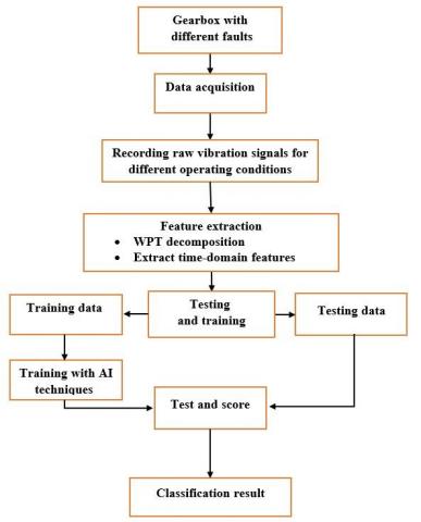
The present study introduces a technique for the fault diagnosis of gears, depending on the method of extraction of features, dimensionality reduction techniques, and artificial intelligence technologies, such as SVM and ANN. Wavelet Packet Transform is utilized for the extraction of features since it is more effective than wavelet transforms for data compression and decomposition. The feature ranking technique, Gain Ratio, is utilized to rank the characteristics of the high-dimensional dataset. The low-ranking characteristics are filtered to form fresh, reduced data subsets. By exploring these techniques and comparing their performance, this research aims to advance the field of gearbox fault detection and pave the way for more reliable and efficient machine health monitoring systems in the manufacturing industry. The flow diagram of the diagnosis method is revealed in Figure 1.
Figure 1. The flow diagram of the diagnosis method
1.1 Wavelet transform
The Wavelet Transform is a powerful and contemporary mathematical tool that has emerged as a highly effective technique for analyzing non-stationary signals. Its unique properties make it particularly well-suited for the analysis of non-stationary vibration signals, which exhibit dynamic and time-varying characteristics. By employing the Wavelet Transform, researchers and engineers can effectively capture and study the intricate patterns and transient behaviors embedded within these complex vibration signals, enabling a more comprehensive and accurate understanding of the underlying phenomena. Contrary to STFT, where the size of the window is constant for the whole signal analysis, the wavelet transform utilizes changeable sizes of windows for the whole sign to obtain a virtuous resolution in both frequency and time. And its opinion is depended upon the signal decomposition into different scales' wavelet coefficients in the time domain. One can divide the class of wavelet transform into (3) types: Wavelet Packet Transform (WPT), continuous wavelet transform (CWT), and discrete wavelet transform (DWT) [13].
1.1.1 Continuous wavelet transform (CWT)
It is defined as follows:
$\hat{f}(a, b)=\int_{-\infty}^{+\infty} f(t) \psi_{a, b}^*(t) \mathrm{d} t$ (1)
Wavelets are therefore defined by:
$\psi_{a, b}(t)=\frac{1}{\sqrt{a}} \psi\left(\frac{t-b}{a}\right), a \in \mathfrak{R}^{*+}, b \in \Re$ (2)
Eq. (1) becomes:
$\hat{f}(a, b)=\frac{1}{\sqrt{a}} \int_{-\infty}^{+\infty} f(t) \psi^*\left(\frac{t-b}{a}\right) \mathrm{d} t$ (3)
where, a and b are the parameters of dilation (scale) and the translation (shift) parameters correspondingly:
$\psi(t)$: The mother wavelet
$\psi^*(t)$: The complex conjugate of $\psi$
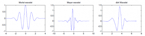
Numerous mother wavelets, like Morlet functions, Daubechies, Meyer, and Haar, can be employed for the detection as well as diagnosis of faults in rotating machinery. Thus, the wavelet transform provides virtuous outcomes when the mother wavelet is cautiously chosen (Figure 2).
1.1.2 Discrete Wavelet Transform (DWT)
It is a continuous wavelet transform (CWT) discretization. Via substituting,
$a=a_0^m$ et $b=n b_0 a_0^m$ with $a_0 \in Z$ et $b_0 \in Z$.
The above expression becomes
$\hat{f}(m, n)=a_0^{-\frac{m}{2}} \int_{-\infty}^{+\infty} f(t) \psi\left(a_0^{-m} t-n b_0\right) \mathrm{d} t$ (4)
The highly usual discretization is dyadic, where a = 2 et b = 1 with m and n integers,
$\hat{f}(m, n)=2^{-\frac{m}{2}} \int_{-\infty}^{+\infty} f(t) \psi\left(2^{-m} t-n\right) \mathrm{d} t$ (5)
An applied form of the discrete wavelet transforms, named Multi-Resolution Analysis (MRA), permits the signal $s(t)$ to decompose at many levels. It consists of introducing the initial signal $s(t)$ into low-pass (L) and high-pass (H) filters. At level one, a pair of vectors $\left(A_1\right.$ and $\left.D_1\right)$ will be determined. Also, the vector elements $\left(A_1\right)$ being named Approximation Coefficients, and the vector elements $\left(D_1\right)$ being named Detail Coefficients $\left(D_2\right)$. The process can be recurrent with $\left(A_1\right)$ at level two, a pair of vectors $\left(A_2\right.$ and $\left.D_2\right)$ will be determined. The procedure of decomposition can be recurrent $j$ times, with $j$ the ultimate no. of levels. The DWT work procedure is displayed in Figure 3.
1.1.3 Wavelet Packet Transform (WPT)
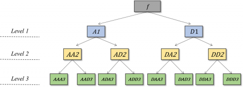
WPT can be considered a distinctive discrete wavelet transform (DWT) format. The DWT easily decomposes the estimate signals, and the WPT is able to capture the info of the two detailed estimate signal constituents (Figure 4). Therefore, the WPT derives further clarified frequency resolution from the decomposed signal. Similar wavelet foundations (i.e., sym, db., and coif) are utilized for the WPT to facilitate the relative analysis with the DWT [14].
The WPT has been confirmed to be effective in the analysis of vibration signals of numerous engineering uses [7]. It decomposes the high-frequency as well as the low-frequency into $2^j$ The band of interval frequency permits better signals' time-frequency localization. For such reason, the WPT is highly suitable for the extraction of features from the frequency domain and the time domain of the vibration signals.
For analyzing the time features in various bands of the frequency of the signal of vibration, the raw signal is decomposed via the decomposition of a j-level wavelet packet. Thus, there's an entire set of $2^j$ packets with the sequence m=1, 2, 3… $2^j$ that being determined. R (j, m) represents the mth node beneath the j level. In the present investigation, the decomposition of a three-level wavelet packet, j = 0, 1, 2, 3, and m = 1, 2, 3…8, as well as the reconstruction of each node of the 3rd level, were taken. This reflects the signal variation with the time in the range [(m-1)/$2^j$ and m/$2^j$] of frequency. The reconstructed signal of every node comprises a characteristic band of frequency reflecting certain fault information.
Figure 2. Examples of mother wavelets [15]
Figure 3. Discrete wavelet transform [16]
Figure 4. Wavelet packet decomposition [14]
1.2 Time-domain statistical features extraction
The time-domain signal can diagnose the fault by analyzing the vibration signals from different conditions. The statistical technique of the time domain is able to give the physical features of the time series data. For example, Widodo [17] employed the features of the time-domain statistical to detect the defects in low-speed bearing, like kurtosis, skewness, standard deviation, and mean. He et al. [18] utilized the statistical parts for diagnosing the faults of gear, containing the MDE, crest factor, and kurtosis. In the present investigation, six statistical features time domains have been employed for analyzing the signal of vibration from various state experiments and are listed in Table 1.
Table 1. The chosen statistical characteristics derived from the time-domain signals
|
Time-Domain Feature |
Equation |
|
Root mean square |
$x_{r m s}=\sqrt{\frac{1}{N} \sum_{i=1}^N x_i^2}$ |
|
Kurtosis |
$x_{k u r}=\frac{1}{N} \sum_{i=1}^N x_i^4$ |
|
Crest factor |
$c_f=\frac{x_p}{x_{r m s}}$ |
|
Variance |
$D_x=\frac{1}{N-1} \sum_{i=1}^N\left(x_i-\bar{x}_i\right)^2$ |
|
Skewness |
$S k=\frac{\frac{1}{N} \sum_{n=1}^N(x[n]-\bar{x})^3}{\sigma^3}$ |
1.3 Feature selection using gain ratio algorithm
The selection of the feature subset is of high significance in the data mining field. The large size of the data makes the testing and training complicated. The selection of important features is the difficulty of selecting a small feature subset that, idyllically, is essential and adequate for describing the idea of the target [19]. The expressions features, variables, and the feature selection objective are to evade choosing very few features or very numerous than is necessary. When very few features are selected, there's a virtuous opportunity that the info included in such features group brings low.
On the other side, when too numerous (irrelevant) features are chosen, the noise influences existing in the majority of real-world data may overshadow the existing info. Therefore, this is an interchange that should be addressed via every technique of the selection of features [20]. In this study, the filter-based feature subset selection method known as the Gain Ratio (GR) was employed to rank and prioritize the features within the utilized dataset.
GR modifies the information gain, reducing bias. The gain ratio considers the branch's no. as well as size if selecting a characteristic. It modifies the gained info by getting the inherent info of splitting into consideration. The inherent info is the entropy of examples distribution into branches, and that means how much information one requires to tell which branch model belongs to. The value of an attribute reduces as inherent information becomes bigger [21].
Gain ratio (Attribute $)=\frac{\text { Gain (Attribute })}{\text { Intrinsic info ( Attribute })}$
After collecting the vibration data and extracting the time domain features from that data, one has a large number of features, and it is possible that some of them are not effective. Therefore, the gain ratio method was used to reduce this data and remove the weak-impact features.
It's too valuable as the features no. of the categorized entities won't influence the SVM performance [22]. This means that no limited number of attributes can be selected as the basis of the diagnosis system. There is no requirement for experts' knowledge of SVM, and no layers are included in the structure of SVM.
2.1 Multiclass classification based on SVM
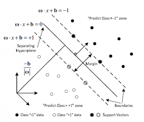
In the context of a binary classification problem, the fundamental concept behind the SVM approach is to construct a hyperplane that serves as the decision boundary. This hyperplane effectively separates the two classes, labeled as negative (-1) and positive (+1), with the maximum possible margin (Figure 5). The margin is defined as the sum of the distances from the hyperplane to the boundaries formed by the nearest data points from each of the two classes. These closest data points, which determine the boundaries, are referred to as the support vectors.
Assume that there's a certain training data set $G=\left\{\left(x_i, y_i\right), i=1 \ldots P\right\}$, every sample $x_i \in R^D$ goes to a class $y_i \in\{+1,-1\}$. The Support Vector Machine hyper-plane can be stated as:
$\omega \cdot x+\mathbf{b}=0$ (6)
where, $\omega$ represents a weight vector, and b represents a bias vector. Therefore, the subsequent decision function can be utilized for classifying every data point (x) in either class (-1) or (+1):
$f(x)=\operatorname{sgn}(\boldsymbol{\omega} \cdot x+\mathbf{b})$ (7)
where, $\operatorname{sgn}(\cdot)$ is the process for finding the value's sign. In relation to (8), the Support Vector Machine-based classifier is:
$f(x)=\operatorname{sgn}\left[\sum_{i=1}^{\mathrm{P}} a_i y_i K\left(x, x_i\right)+\mathbf{b}\right]$ (8)
It is subject to:
$\sum_{i=1}^l \alpha_i y_i=0$ (9)
where, $\alpha_i \geq 0$ represents a Lagrange multiplier, $K\left(x, x_i\right)$. It's the kernel function.
The kernel function employed in SVM performs a mapping of the input vectors into a higher-dimensional feature space through a nonlinear transformation. This mapping enables the construction of a separating hyperplane, thereby rendering the data linearly separable in the feature space, even though the original input vectors may not be linearly separable in the input space [23]. One of the widely used kernel functions for SVMs is the Radial Basis Function (RBF). The popularity of the RBF kernel stems from its similarity to the K-Nearest Neighbor (K-NN) algorithm. It combines the advantages of K-NN while addressing the issue of space complexity, as RBF kernel SVMs only need to store the support vectors during training rather than the entire dataset. The RBF kernel is considered to exhibit highly accurate, reliable, and effective performance in practical applications [24]. Figure 5 illustrates the classification process using an SVM.
The gearbox fault categorization is a multiclass problem. Thus, a multiclass SVM classifier is designed. Selecting a suitable strategy for categorization is a crucial topic in multiclass categorization, and much effort was conducted on such matters [25]. For the purpose of assessing the condition of the gearbox under examination in this research, a multiclass Support Vector Machine (SVM) classifier with a radial basis function (RBF) kernel was utilized.
Figure 5. SVM classification [26]
Artificial Intelligence (AI), as defined by John McCarthy, is "the science and engineering of creating intelligent machines" [27]. Artificial Neural Networks (ANNs), a branch of AI, draw inspiration from the design and functioning of the human brain. ANNs possess remarkable capabilities in pattern recognition, classification, data interpretation, and function approximation. They provide a nonlinear, parameterized mapping between input data and output data. ANNs consist of interconnected networks organized into layers of input neurons, hidden neurons, and output neurons. These layers are linked through transfer functions, while adjustable weights are assigned to the neurons. ANNs exhibit a diverse range of architectures and topologies, each tailored to specific applications and requirements. The power of ANNs lies in their ability to learn from data and adapt their internal parameters, enabling them to capture intricate patterns and relationships within the data. Through a process of training on representative examples, ANNs can generalize their learning and make accurate predictions or decisions on previously unseen data. This adaptability and robustness have made ANNs invaluable tools in various domains, including pattern recognition, signal processing, control systems, and data analysis. Feed-forward multilayer perceptions are the most frequently utilized networks in fault detection (MLP).
Figure 6 shows an MLP network with layers $i, j$, and $k$ and interconnection weights $W_{i j}$ and $W_{j k}$ between the layers of the neurons. The originally given weights are continually adjusted during training. The outputs that MLP predicted are compared to the ones that actually happened, and the mistakes are backpropagated (from right to left in Figure 6). The weights are modified or rectified based on this approach, and mistakes are reduced.
Figure 6. The schematic diagram for 3-layered MLP [28]
4.1 Experiment setup
The test rig is designed for experimental testing on gears, as shown in Figure 7, which can simulate the most common faults in gear teeth. It was utilized to perform a wide investigational monitoring of the various failure modes of the gear. The two-stage helical gearbox was used, and its details are explained in detail in Table 2. A load generator and an induction motor connect both gearboxes via flexible couplings. Such preparation permits various load states to be imposed upon the gearboxes of the test. The assembly of the test rig is driven via a 1.1 kW (1.5 hp) AC motor (1472 rpm), whereas the servomotors were utilized for applying various states of load upon the regime. The accelerometer was strategically positioned on the gearbox housing in the vertical direction, specifically in close proximity to the potential damage site for this particular test. Placing the sensor as close as possible to the expected damage sites is a recommended practice. This approach ensures that the sensor captures the most relevant and accurate data related to potential faults or abnormalities in the gearbox [29].
In addition to having the test device, there are tools to complete the task, the most important of which are the accelerometer and Data Acquisition System (DAQ) used to analyze that data. Table 3 summarizes the tools used in this work and their respective functions.
Figure 7. Test rig for gearbox fault diagnosis
Figure 8. Simulated gear faults
Table 2. Two-stage helical gearbox details
|
Description |
1 Stage |
2 Stages |
||
|
Pinion |
Gear |
Pinion |
Gear |
|
|
No of teeth |
|
|
|
|
|
Rotation speed (rpm) |
1472 |
530 |
530 |
98 |
|
Meshing frequency (Hz) |
540 |
107 |
||
|
Gear ratio |
2.7 |
5.4 |
||
In the current investigation, the faults of the gear were analyzed. Four kinds of gear faults were utilized in the experiments: Broken gear teeth, cracked teeth, worn teeth, and missed teeth (see Figure 8). The test rig was set to different operating conditions with four speeds (570,870,1170 and 1472 rpm) and a load of 10 NM. Table 4 evinces a thorough description of the faults.
Table 3. Accelerometer and data acquisition system
|
Tools |
Type |
Function |
|
Accelerometer |
IEPE Type CTC102-1A |
Vibration measurement |
|
Data Acquisition System/Hardware |
NI USB-4431 from National Instruments |
Acquire data from the accelerometer |
|
Data Acquisition System/Software |
LabVIEW Program |
Manages data collection and has necessary capabilities, including wavelet analysis and time-domain |
Table 4. Description of each fault condition of the gearbox
|
Test Number |
Condition |
Fault Code |
|
1 |
Healthy |
H |
|
2 |
Wear teeth |
W |
|
3 |
Crack tooth |
C |
|
4 |
Broken teeth |
B |
|
5 |
Missed tooth |
M |
Figure 9. A sample of the developed LabVIEW program
Figure 10. The vibration signals from the first speed of the gearbox with five conditions
4.2 Data acquisition
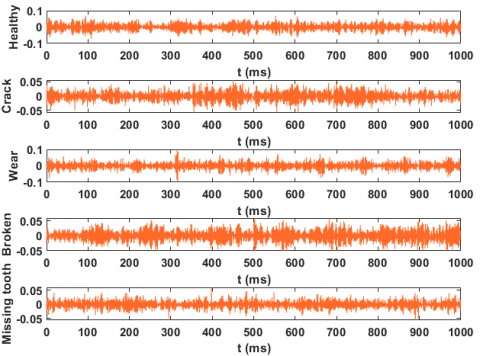
In this study, the test gearbox was operated under the most demanding operating conditions. It was observed that the highest frequency present in the system did not exceed 600 Hz. Consequently, the sampling rate was set to 2048 ($2^{11}$) samples per second, in accordance with the Nyquist sampling theorem, which states that the sampling rate should be at least twice the highest frequency component in the signal to avoid aliasing. Due to the inherent noise that accompanies such operating conditions, it was crucial to avoid an excessively high sampling rate, as this would lead to redundancy in the signal representation and result in increased noise levels in the recorded signal. Therefore, the chosen sampling rate of 2048 Hz strikes a balance between capturing the relevant frequency components while minimizing the impact of noise on the recorded vibration signal. A Data Acquisition System was employed to acquire the vibration signals from the gearbox through a sensor. A dedicated system was developed using the LabVIEW programming environment to record the raw vibration signals. Subsequently, the wavelet transform method was applied to decompose and reconstruct the original signal, enabling the extraction of relevant features. The classification system then utilized these extracted features to facilitate the identification and categorization of potential faults. Figure 9 manifests a simple system for the LabVIEW program, where the original signal is processed and reconstructed by a wavelet packet, and then features are extracted from it and stored. The vibration signal was acquired for five operation conditions (One healthy and four different faults). Two hundred unceasing measurements were registered for every situation. The registered length of time length of every measure was (0.5 sec), and the no. of data was 1024 ($2^{10}$), and the rate of sampling was 2048 ($2^{11}$) Hz. Also, the raw signals of the vibration of five states are schemed in Figure 10.
5.1 Methodology processes
The flow diagram of the fault diagnosis of gear is elucidated in Figure 1. It comprises (4) sections: Acquisition of data, extraction of feature, selection of feature, and training, as well as testing for the diagnosis of the fault. The extracted feature throughout the statistical computation of WPT in addition to the time domain. The Wavelet Packet Transform is too appropriate for the extraction of features from the time- and frequency-domain of the signals of vibration. Furthermore, feature extraction techniques are employed to eliminate redundant and irrelevant information from the acquired data. The optimal set of features is then selected through a feature selection method, which aims to reduce the volume of raw data while simultaneously enhancing the classification accuracy. Ultimately, the SVM is utilized to classify the faults in the gearbox. The training and testing processes are carried out using artificial intelligence techniques, specifically the SVM and ANN. Within the test step, the training model in the present work was used to test the five gear conditions, which contain the usual conditions and four gear faults. The results showed that this method reaches the ideal performance.
5.2 Feature extractions based on WPT and time domain analysis
In this study, the maximum frequency in the system does not exceed 540 Hz. According to the sampling rate, the frequency range of raw signal R is within [0, 1024 HZ]. Wavelet packets were decomposed into three levels, as shown in Figure 11.
The main feature extraction steps based on WPT are denoted as follows:
Step 1: Daubechies-4 (dB-4) wavelet was employed to decompose the three-level raw signals. Daubechies wavelets have gained significant popularity in the field of rotating machine fault diagnosis, specifically db4 [30].
Step 2: Take the reconstruction signal in every node of the 3rd level to extract the features in the various frequency bands of the vibration signal. This level was chosen because the vibration signal analysis at the third level covers a wide range of frequencies present in the system. Therefore, in this work, eight re-construction signals R31, R32, R33, R34, R35, R36, R37, R38 (Green boxes in Figure 11) were determined. R denotes the raw signal; R31 denotes the level 3 node 1. Figure 12 shows how to reconstruct the raw vibration signal into eight reconstructed signals by Wavelet Packet Transform of the healthy state of the gearbox.
Step 3: Calculate 5 statistical feature factors of the time domain for the (8) reconstruction signals. Two hundred features were obtained for each of the time domain statistical factors. Table 5 shows the total number of statistical features extracted for each case after the reconstruction signal by applying (WPT) method.
Figure 11. Wavelet packets were decomposed into three levels
Figure 12. Raw and reconstruction signals for a healthy gearbox
Table 5. Statistical features of the time domain
|
Statistical |
No. of Statistical |
No. of All Features |
|
RMS |
8 |
1600 |
|
KU |
8 |
1600 |
|
SK |
8 |
1600 |
|
VA |
8 |
1600 |
|
CF |
8 |
1600 |
|
TOTAL |
40 |
8000 |
Based on the information provided in Table 5, the number of statistical features for each individual case is represented by a matrix with dimensions of 200 rows and 40 columns. To obtain the dataset for all cases, these individual case matrices are combined, resulting in a larger matrix with dimensions of 4000 rows and 40 columns. This is because there are a total of 20 cases (200 rows×20 cases = 4000 rows), and each case has 40 features (columns). Consequently, the overall dataset for all cases consists of a matrix with 4000 rows (representing the combined data from all 20 cases) and 40 columns (representing the 40 features extracted for each case). The total number of features in the dataset can be calculated by multiplying the number of rows (4000) by the number of columns (40), which yields 160,000 features. In summary, the dataset for all cases is a matrix of dimensions 4000×40, and the total number of features in the dataset is 160,000.
5.3 Feature selection and classification
Data mining has recently appealed much care in the community, converting big data quantities into valuable information and awareness. It is a procedure that utilizes mathematical, statistical, machine learning, and artificial intelligence methods for extracting and identifying valuable info and correlated awareness from different big databases [31].
Open-source data mining software is used to construct categorization algorithms on the datasets. The utilized software is a tool from ORANGE founded upon phyton programming [32]. ORANGE is a valuable tool for data mining for optical programming as well as the analysis of explorative data. It can also be conducted in phyton. The multiple constituents of ORANGE are recognized as widgets. Such data mining tools support Linux, macOS, and Windows. Another advantage of this program is the selection of the influential features from the primary data set and the classification procedure in the same process. As a result, the number of features can be selected from the data set to be trained and tested under the accuracy of the classification.
Figure 13. Flow diagram for feature selection and classification processing
In this work, 4000 samples* 40 features were collected for all cases (H, W, C, B, and M). The influencing features were selected using the Gain Ratio method, and the classification was done using SVM and ANN classifiers. The Gain Ratio method divides the features into the data set according to the attribute's intrinsic information, reducing the features that contain unimportant information. The data set was split into a training data set of 70% (2800 samples) and a testing data set of 30% (1200 samples) for verifying the classifier. The feature selection and classification process flow diagram are shown in Figure 13. It is implemented using the program ORANGE.
Tables 6 and 7 present the performance evaluation of the Support Vector Machine (SVM) model. Table 6 displays the results before applying the feature selection strategy, while Table 7 shows the results after employing the feature selection approach. When considering all 40 features, the base SVM model achieved a classification accuracy of 91%. However, after implementing the feature selection technique, which reduced the number of features to 16, the SVM model demonstrated improved performance with a higher classification accuracy of 96%. In addition to the increased classification accuracy, the precision metric also improved, rising from 86% to 91% after feature selection. Similarly, the recall metric saw a substantial improvement, increasing from 89% to 97%. Furthermore, the Area Under the Curve (AUC) metric, which evaluates the model's overall performance, exhibited an enhancement, increasing from 98% to 99% after the feature selection process. These results highlight the positive impact of the feature selection strategy, which not only reduced the dimensionality of the data but also improved the overall performance of the SVM model across multiple evaluation metrics, including classification accuracy, precision, recall, and AUC.
Table 6. SVM Model results’ evaluation before feature ranking
|
Model |
AUC % |
CA % |
Precision % |
Recall % |
|
SVM |
98 |
91 |
86 |
89 |
Table 7. SVM Model results’ evaluation after feature ranking
|
Model |
AUC % |
CA % |
Precision % |
Recall % |
|
SVM |
99 |
96 |
91 |
97 |
Figure 14 shows how the SVM model has predicted 99.6% of the state of health as healthy and 0.4% as a worn tooth. Where the balls on the right of Figure 14 represent the prediction result of the test data for the case of healthy teeth, and the balls on the left represent the test data for the other cases. By describing the colors in the figure, the green balls represent the condition of healthy teeth, while the other colors represent the other conditions. Since the accuracy of data classification for the condition of healthy teeth amounted to 99.6%, so we note that most of the balls in the condition of healthy teeth are green, which represents 99.6% of the test data for the condition of healthy teeth, While the yellow ball with the green balls on the right of the figure represents the classification error percentage of 0.8%, which indicates the worn tooth.
In this work, a classification of gearbox faults was carried out using artificial intelligence techniques, and two classifiers, SVM and ANN, were used in order to identify the difference between these techniques and to choose the best model for the classification. The same procedures that were applied to the classifier SVM are now applied to the ANN classifier, and the effect of feature selection on the classification process is demonstrated. Tables 8 and 9 show the effect of applying feature selection on classification by ANN. Where we also notice an increase in classification accuracy from (96) to (98) and an increase in each of AUC, Precision, and Recall after the feature selection process, and that the optimal number of features to obtain the best classification of faults is 16 features.
Figure 14. Scatter plot for predicting crack tooth case by SVM model
Figure 15. Confusion matrices of classification by ANN model
Table 8. ANN Model results’ evaluation before features ranking
|
Model |
AUC % |
CA % |
Precision % |
Recall % |
|
ANN |
99 |
96 |
92 |
95 |
Table 9. ANN Model results’ evaluation before features ranking
|
Model |
AUC % |
CA % |
Precision % |
Recall % |
|
ANN |
100 |
98 |
98 |
98 |
The confusion matrix in Figure 15 shows how to classify the five healthy and defective states of the gearbox under different speeds and constant load by the ANN model. The horizontal axis indicates the predicted values and the vertical axis displays the actual values. The goal is to have as many correct forecasts as possible (lots of points in the diagonal). Each row displays how the machine learning model trained on the training set predicts the data of the testing set for each case. The confusion matrix displays the categorization by ANN model outcomes for the test dataset. The results reveal that the classification accuracy of the health and fault states of the gearbox approaches 98%. Through the result, we notice that the worn tooth occupies the highest classification accuracy of 99.6%, followed by the healthy tooth and broken tooth, with the accuracy of 99.2% and 98.3%, respectively. It was the least accurate classification of the crack tooth, followed by the missing tooth, with a classification accuracy of 98% and 97.9%, respectively.
Through Tables 7 and 9, it can be seen that the classification accuracy of the model ANN is higher than that of the model SVM due to the noise present in the vibration signal, as it reduces the performance of SVM, and this is identical to what was mentioned by Mohd Ghazali and Rahiman [33]. On the other hand, we notice that the training time for the ANN classifier is longer than the training time for the SVM classifier, as it depends on the number of iterations.
These findings provide a somewhat accurate description of the gearbox state. It suggests that the SVM and ANN classifiers have successful data training. It should be mentioned that the accuracy of the machine learning method frequently depends on the quality of the features; in this instance, features that are excellent condition indicators are extracted using the domain knowledge of the physics of defects.
The findings of this study hold significant practical implications for the field of gearbox fault diagnosis. By applying a combination of Wavelet Packet Transform (WPT), computation of time domain statistical features, information gain ratio technique (GR), and artificial intelligence techniques (SVM and ANN), the study demonstrates the effectiveness of integrating traditional vibration signal analysis with advanced machine learning methods for fault diagnosis in gearboxes.
Overall, the study's results contribute to advancing the effectiveness and efficiency of gearbox fault diagnosis, offering practical solutions to industries seeking improved condition monitoring and predictive maintenance strategies. By leveraging the proposed methodology, companies can minimize unplanned downtime, optimize maintenance schedules, and ensure the safe and reliable operation of critical rotating machinery in various industrial settings.
[1] Yesilyurt, I. (2004). The application of the conditional moments analysis to gearbox fault detection—A comparative study using the spectrogram and scalogram. NDT & E International, 37(4): 309-320. https://doi.org/10.1016/j.ndteint.2003.10.005
[2] Baydar, N., Ball, A. (2003). Detection of gear failures via vibration and acoustic signals using wavelet transform. Mechanical Systems and Signal Processing, 17(4): 787-804. https://doi.org/10.1006/mssp.2001.1435
[3] Peng, Z.K., Chu, F.L. (2004). Application of the wavelet transform in machine condition monitoring and fault diagnostics: A review with bibliography. Mechanical Systems and Signal Processing, 18(2): 199-221. https://doi.org/10.1016/S0888-3270(03)00075-X
[4] Sung, C.K., Tai, H.M., Chen, C.W. (2000). Locating defects of a gear system by the technique of wavelet transform. Mechanism and Machine Theory, 35(8): 1169-1182. https://doi.org/10.1016/S0094-114X(99)00045-2
[5] Xian, G.M., Zeng, B.Q. (2009). An intelligent fault diagnosis method based on wavelet packer analysis and hybrid Support Vector Machines. Expert Systems with Applications, 36(10): 12131-12136. https://doi.org/10.1016/j.eswa.2009.03.063
[6] Samanta, B. (2004). Gear fault detection using artificial neural networks and Support Vector Machines with genetic algorithms. Mechanical Systems and Signal Processing, 18(3): 625-644. https://doi.org/10.1016/S0888-3270(03)00020-7
[7] Hu, Q., He, Z., Zhang, Z., Zi, Y. (2007). Fault diagnosis of rotating machinery based on improved wavelet package transform and SVMs ensemble. Mechanical Systems and Signal Processing, 21(2): 688-705. https://doi.org/10.1016/j.ymssp.2006.01.007
[8] Widodo, A., Yang, B.S. (2007). Application of nonlinear feature extraction and Support Vector Machines for fault diagnosis of induction motors. Expert Systems with Applications, 33(1): 241-250. https://doi.org/10.1016/j.eswa.2006.04.020
[9] Yang, B.S., Han, T., Hwang, W.W. (2005). Fault diagnosis of rotating machinery based on multiclass Support Vector Machines. Journal of Mechanical Science and Technology, 19: 846-859. https://doi.org/10.1007/BF02916133
[10] Lei, Y., He, Z., Zi, Y., Chen, X. (2008). New clustering algorithm-based fault diagnosis using compensation distance evaluation technique. Mechanical Systems and Signal Processing, 22(2): 419-435. https://doi.org/10.1016/j.ymssp.2007.07.013
[11] Huang, C.L., Wang, C.J. (2006). A GA-based feature selection and parameters optimizationfor Support Vector Machines. Expert Systems with Applications, 31(2): 231-240. https://doi.org/10.1016/j.eswa.2005.09.024
[12] Priyadarsini, R.P., Valarmathi, M.L., Sivakumari, S. (2011). Gain ratio based feature selection method for privacy preservation. ICTACT Journal on Soft Computing, 1(4): 201-205. https://doi.org/10.21917/ijsc.2011.0031
[13] Boudiaf, A., Moussaoui, A., Dahane, A., Atoui, I. (2016). A comparative study of various methods of bearing faults diagnosis using the case Western Reserve University data. Journal of Failure Analysis and Prevention, 16(2): 271-284. https://doi.org/10.1007/s11668-016-0080-7
[14] Hu, J., Liu, B., Peng, S. (2019). Forecasting salinity time series using RF and ELM approaches coupled with decomposition techniques. Stochastic Environmental Research and Risk Assessment, 33: 1117-1135. https://doi.org/10.1007/s00477-019-01691-1
[15] Sun, Q., Tang, Y. (2002). Singularity analysis using continuous wavelet transform for bearing fault diagnosis. Mechanical Systems and Signal Processing, 16(6): 1025-1041. https://doi.org/10.1006/mssp.2002.1474
[16] Castejón, C., Gómez, M.J., Garcia-Prada, J.C., Ordonez, A., Rubio, H. (2015). Automatic selection of the WPT decomposition level for condition monitoring of rotor elements based on the sensitivity analysis of the wavelet energy. International Journal of Acoustics and Vibration, 20(2): 95-100.
[17] Widodo, A., Kim, E.Y., Son, J.D., Yang, B.S., Tan, A.C., Gu, D.S., Choi, B., Mathew, J. (2009). Fault diagnosis of low speed bearing based on relevance vector machine and Support Vector Machine. Expert Systems with Applications, 36(3): 7252-7261. https://doi.org/10.1016/j.eswa.2008.09.033
[18] He, Q., Kong, F., Yan, R. (2007). Subspace-based gearbox condition monitoring by kernel principal component analysis. Mechanical Systems and Signal Processing, 21(4): 1755-1772. https://doi.org/10.1016/j.ymssp.2006.07.014
[19] Kira, K., Rendell, L.A. (1992). A practical approach to feature selection. In Machine Learning Proceedings 1992, pp. 249-256. Morgan Kaufmann. https://doi.org/10.1016/B978-1-55860-247-2.50037-1
[20] Piramuthu, S. (2004). Evaluating feature selection methods for learning in data mining applications. European Journal of Operational Research, 156(2): 483-494. https://doi.org/10.1016/S0377-2217(02)00911-6
[21] Han, J., Kamber, M., Pei, J. (2001). Data mining concepts and techniques, Morgan Kaufmann Publishers. San Francisco, CA, 335-391.
[22] Poyhonen, S., Negrea, M., Arkkio, A., Hyotyniemi, H., Koivo, H. (2002). Support vector classification for fault diagnostics of an electrical machine. In 6th International Conference on Signal Processing, Beijing, China, pp. 1719-1722. https://doi.org/10.1109/ICOSP.2002.1180133
[23] Vapnik, V. (1999). The Nature of Statistical Learning Theory. Springer Science & Business Media.
[24] Tyagi, CS (2008). A comparative study of SVM classifiers and artificial neural networks application for rolling element bearing fault diagnosis using wavelet transform preprocessing. International Journal of Mechanical and Mechatronics Engineering, 2(7): 904-912.
[25] Hsu, C.W., Lin, C.J. (2002). A comparison of methods for multiclass Support Vector Machines. IEEE Transactions on Neural Networks, 13(2): 415-425. https://doi.org/10.1109/72.991427
[26] Lu, D., Qiao, W. (2014). Fault diagnosis for drivetrain gearboxes using PSO-optimized multiclass SVM classifier. In 2014 IEEE PES General Meeting| Conference & Exposition, National Harbor, MD, USA, pp. 1-5. https://doi.org/10.1109/PESGM.2014.6939892
[27] McCarthy, J. (1979). Ascribing mental qualities to machines. Technical Report, Stanford University. Computer Science Department, pp. 161-195.
[28] Bouboulas, A., Nikolakopoulos, P., Anifantis, N. (2022). Prediction of crack depth and position in vibrating beams using artificial neural networks. Diagnostyka, 23(3): 2022307. http://doi.org/10.29354/diag/154758
[29] Farrar, C.R., Worden, K. (2012). Structural Health Monitoring: A Machine Learning Perspective. John Wiley & Sons.
[30] Zhang, Z., Wang, Y., Wang, K. (2013). Intelligent fault diagnosis and prognosis approach for rotating machinery integrating wavelet transform, principal component analysis, and artificial neural networks. The International Journal of Advanced Manufacturing Technology, 68: 763-773. https://doi.org/10.1007/s00170-013-4797-0
[31] Ishak, A., Siregar, K., Ginting, R., Afif, M. (2020). Orange software usage in data mining classification method on the dataset lenses. IOP Conference Series: Materials Science and Engineering, 1003(1): 012113. https://doi.org/10.1088/1757-899X/1003/1/012113
[32] Oktanisa, I., Supianto, A.A. (2018). Perbandingan Teknik Klasifikasi Dalam Data Mining Untuk Bank Direct Marketing. Jurnal Teknologi Informasi dan Ilmu Komputer, 5(5): 567-576. https://doi.org/10.25126/jtiik.201855958
[33] Mohd Ghazali, M.H., Rahiman, W. (2021). Vibration analysis for machine monitoring and diagnosis: A systematic review. Shock and Vibration, 2021: 1-25. https://doi.org/10.1155/2021/9469318