Asifa Mohammed*![]() | Aseel A. Alhamdany
| Aseel A. Alhamdany![]() | Ali Y. Khenyab
| Ali Y. Khenyab![]()
© 2024 The authors. This article is published by IIETA and is licensed under the CC BY 4.0 license (http://creativecommons.org/licenses/by/4.0/).
OPEN ACCESS
Understanding the erosion characteristics of different pipe materials is of paramount importance in the field of pipeline transportation due to its critical role in maintaining operational efficiency and safety. However, erosion caused by entrained particles during fluid flows poses a significant challenge to pipeline integrity. This study employs Computational Fluid Dynamics (CFD) to comprehensively analyze and compare the erosion behaviors of stainless steel XS80S and steel XS80 pipes with 90° elbows. The investigation focuses on turbulent oil and sand particle transportation conditions, enabling the prediction of erosion rate distribution and particle trajectories, particularly within the elbow region. The results highlight the superior erosion resistance of stainless steel XS80S over steel XS80 across various simulation models. The study underscores the significance of material selection in combating erosion and enhancing pipeline integrity. The XS80S pipes performed better than the XS80 Pipes. The maximum Dpm Erosion Rate Finnie model for the XS80S and XS80 pipes were 8.62 E-25 mm3 kg-1 and 9.17 E-25 mm3 kg-1, respectively; for the McLaury model they were 2.94E-24 mm3 kg-1 and 3.10E-24 mm3 kg-1, respectively; for the Oka model they were 5.68E-26 mm3 kg-1 and 6.75E-26 mm3 kg-1, respectively. The maximum Dpm Accretion Rate for the XS80S and XS80 pipes were 2.01E-17 mm3 kg-1 and 2.06E-17 mm3 kg-1, respectively. Furthermore, the investigation sheds light on the vulnerabilities of the elbow region within pipelines, providing insights into targeted design modifications and maintenance protocols. This research advances the understanding of erosion mechanisms, fluid dynamics, and material performance, offering actionable insights for pipeline industry stakeholders. The findings lay the groundwork for future research avenues and contribute to the evolution of corrosion management practices.
erosion modeling, Computational Fluid Dynamics (CFD), pipeline integrity, material selection, erosion resistance, elbow region vulnerability
Pipeline transport is a critical mode of transportation in the crude oil and natural gas industry due to its remarkable efficiency and safety [1, 2]. However, despite its economic benefits, pipeline transport faces several challenges. Among these challenges, the most significant is the erosion of pipeline internal surfaces caused by entrained particles during fluid flows [3-19]. Erosion-induced wear within pipelines, caused by the interaction between fluid and solid particles, poses a critical issue for the oil and gas sector. The damage accrued over time can compromise the structural integrity of pipelines, leading to leaks, disruptions in supply, and potentially catastrophic incidents. In addition, erosion not only results in costly repairs but also poses environmental and safety risks. Solid particles tend to accumulate on the walls of bent pipes due to pressure drops, resulting in erosion issues and, eventually, oil leakage. Moreover, the chemical composition of transported fluids plays a significant role in the corrosion process [4]. Advancements in simulation technology have facilitated the understanding of such phenomena [20]. Many companies have recently transitioned to utilizing Computational Fluid Dynamics (CFD) to mitigate erosion wear on machinery and pipeline components. The CFD technique has been employed in numerous studies to predict pipeline erosion under various operational conditions [5, 6].
To address these challenges, this study employs Computational Fluid Dynamics (CFD) to investigate and compare the erosion characteristics of two distinct pipe materials: stainless steel XS80S and steel XS80. The research aims to provide insights into the erosion behaviors of these materials under turbulent oil and sand particle transportation conditions, particularly within the context of 90° elbows. Understanding how different materials respond to erosion is crucial for enhancing pipeline design, material selection, maintenance practices, and overall industry efficiency.
This Research Focus and Hypothesis seeks to address the gap in understanding the erosion characteristics of pipeline materials, specifically stainless steel XS80S and steel XS80, in turbulent fluid flow conditions. The primary research question is: How do the erosion behaviors of these materials differ under the influence of entrained particles, and how can this knowledge be utilized to improve pipeline integrity and operational efficiency?
The significance of this research lies in its potential to revolutionize the way pipeline erosion is understood and managed. By comprehensively analyzing erosion behaviors and comparing two distinct materials, the study aims to contribute valuable insights to pipeline design, material selection, and maintenance practices. These insights are crucial for mitigating erosion-induced damages, extending pipeline lifespans, reducing maintenance costs, and maintaining the safety and reliability of oil and gas transportation networks. The pipe design adheres to ASME/ANSI B 36.10 Welded and Seamless Wrought Steel Pipe and ASME/ANSI B36.19 Stainless Steel Pipe standards [16-18]. The design process was executed using Solidworks software, version 2016, while the modeling and simulation process utilized Ansys software, version 2018.
Extensive investigations have focused on pipeline elbows. For example, Adedeji and Duarte [7] employed an erosion-coupled dynamic mesh approach to investigate surface distortion in a conventional 90° elbow under different wall conditions, comparing computational results with actual data. Duarte and de Souza [8] employed the erosion-coupled dynamic lattice approach methodology, significantly reducing CPU time and enabling more rapid and precise prediction of erosion distortion. Zhang et al. [9] explored the erosion characteristics of bends with corrosion defects using CFD. The findings indicated that the highest erosion rate occurred when the faulty region was at a 55° angle to the elbow. Xu et al. [10] demonstrated that the erosion rate of the elbow decreases with reduced elbow pressure subsidence and turbulent kinetic energy, introducing a model featuring an arched plate to prevent erosion. Sedrez and Shirazi [11] evaluated the effects of gravity and bending direction on corrosion under various conditions and with multiple pipes, highlighting the substantial impact of gravity direction on corrosion rates. For the Limitations and Prior Researches Gap While prior studies have explored various aspects of pipeline erosion, limited research has specifically focused on the distinct erosion behaviors of different materials, especially in the context of 90° elbows. This study addresses this gap by providing a comprehensive comparison of stainless steel XS80S and steel XS80. By doing so, it aims to uncover nuances in material performance that have been previously overlooked, shedding light on how material selection can influence erosion dynamics.
This section delves into the mathematical framework that underlies this study, introducing essential equations and models that are crucial for comprehending fluid flow, erosion, and turbulence in pipelines. These mathematical tools have been chosen for their relevance and importance in addressing the central questions of research. The chosen equations and models were selected based on their established use and relevance in fluid dynamics and erosion studies. The fluid flow in pipes model allows for the calculation of pressure drop, essential for understanding the hydraulic performance of pipelines. The erosion modeling equations enable the estimation of erosion rates, which is crucial for assessing the erosion-induced wear on pipeline surfaces. Lastly, the turbulence flow model provides insights into the behavior of turbulent fluids in the pipeline system, aiding in the analysis and prediction of flow patterns and turbulence effects.
By incorporating these equations and models into the research, can gain a comprehensive understanding of fluid flow, erosion dynamics, and turbulent behavior within the pipelines, thus contributing to the investigation of erosion-related issues and providing valuable insights for pipeline design, material selection, and maintenance practices.
2.1 Fluid flow in pipes model
The Darcy-Weisbach equation plays a pivotal role in analysis of pressure drop during fluid flow within pipes. This equation's significance lies in its ability to incorporate various variables, including density, flow rate, pipe diameter, and friction factor. By employing this equation, we gain insights into pressure distribution and hydraulic performance, allowing to grasp the impacts of friction and other factors on fluid flow behavior. The Darcy-Weisbach equation is integral to quantifying the intricate dynamics of fluid movement within pipelines.
The Darcy-Weisbach equation may be used to calculate the pressure drop in fluid mechanics as follows [12]:
$\Delta P=\frac{8 \rho f L_T}{\pi^2 D^3} Q^2$ (1)
where, ∆P: Pressure drop [K. Pa]; ρ: Fluid density $\left[\frac{\mathrm{kg}}{\mathrm{m}^3}\right]$; Q: Flow rate $\left[\frac{\mathrm{kg}}{\mathrm{s}}\right]$; D: Pipe diameter [m]; LT: The total length of the pipe [m]; f: Darcy friction factor.
$Q=\frac{\pi D^2}{4} V$ (2)
The dimensionless Reynolds number (Re) determines the flow's properties:
$R_e=\frac{V D \rho}{\mu}$ (3)
where, V: The average velocity $\left[\frac{m}{s}\right]$; μ: Dynamic viscosity [pa.s].
The Colebrook equation may be used to determine Darcy friction factor (f) for turbulent flow, where Re>4000:
$\frac{1}{\sqrt{f}}=-2 \log \log \left(\frac{e}{3.7 D}+\frac{2.51}{R_e \sqrt{f}}\right)$ (4)
2.2 Erosion modeling
The erosion modeling in this study aims to predict the rate of erosion caused by the impact of particles on the internal surfaces of the pipeline. Eq. (5) presents a relationship between the erosion rate at a specific impact angle and the erosion rate at a 90° angle. The impact angle function (fα) in Eq. (7) quantifies the influence of the impact angle on the erosion rate. The erosion rate at a 90° angle is determined by Eq. (6), which considers various factors such as fluid density, particle properties, velocities, sizes, and material hardness. These equations enable the estimation of erosion rates and provide insights into the erosive wear of different materials under specific conditions [13, 14].
$E_\alpha=E_{90} f_\alpha$ (5)
where, Eα: The erosion rate at the impact angle [mm3kg-1], E90: The erosion rate at a 90° angle [mm3kg-1], fα: The impact angle function.
$E_{90}=10^{-9} \rho_w K\left(\alpha H_V\right)^{b k_1}\left(\frac{V_P}{V^*}\right)^n\left(\frac{d_P}{d^*}\right)^{k_1}$ (6)
$f_\alpha=(\sin \sin \alpha)^{n 1}\left(1+H_V(1-\sin \sin \alpha)\right)^{n 2}$ (7)
$n=2.3\left(H_V\right)^{0.038}$ (8)
$n_1=0.71\left(H_V\right)^{0.14}$ (9)
$n_2=2.4\left(H_V\right)^{-0.94}$ (10)
where,
ρw: Density of the target material $\left[\frac{\mathrm{kg}}{\mathrm{m}^3}\right]$, K, k1 are constant and exponent, respectively, which take arbitrary units and are determined by the properties of the particle (type of particle), α: Impact angle, b: The load relaxation ratio, dP: Particle size [μm], d*: The reference particle size [μm], VP: The particle velocity [m/s], V*: The reference velocity [m/s], HV: The Vickers hardness of the material [GPa], n, n1, n2: Constants dependent on the hardness of the material.
2.3 The turbulence flow model
The turbulence flow model used in this research addresses the behavior of turbulent fluids, which is crucial for understanding the complex flow patterns and predicting the turbulence-induced effects. Eqs. (11) and (12) represent the momentum conservation and continuity equations, respectively. These equations describe the motion of fluid and ensure mass conservation within the flow. Additionally, Eqs. (13) and (14) introduce the turbulence model, specifically the transport equations for turbulent kinetic energy (K) and turbulent dissipation rate (ω). These equations account for the effect of turbulence on fluid flow and provide insights into the turbulent characteristics of the fluid within the pipeline.
The momentum conservation and continuity equations [15] are:
$\begin{aligned} & \rho \frac{\partial U}{\partial t}+\rho U \cdot \underline{V} U+\underline{V} \cdot\left(\rho u^{\prime} \times u^{\prime}\right) \\ = & -\underline{V} P+\underline{V} \mu\left(\underline{V} U+(\underline{V} U)^T\right)+F\end{aligned}$ (11)
$\rho \underline{V} U=0$ (12)
where, U indicates the average velocity.
The turbulence model is as follows:
$\begin{gathered}\rho \frac{\partial K}{\partial t}+\rho u \cdot \underline{V} K \\ =\left(P_K-\rho \beta^* K \omega+\underline{V}\left(\left(\mu+\sigma^* \mu_T\right) \underline{V} K\right)\right)\end{gathered}$ (13)
$\begin{gathered}\rho \frac{\partial \omega}{\partial t}+\rho u \cdot \underline{V} \omega \\ =\left(\alpha \frac{\omega}{K} P_K-\rho \beta \omega^2+\underline{V}\left(\left(\mu+\sigma \mu_T\right) \underline{V} \omega\right)\right)\end{gathered}$ (14)
where,
$\mu_T=\rho \frac{K}{\omega}, \alpha=\frac{13}{25}, \beta=\beta_o F_\beta, \beta^*=\beta_o{ }^* F_\beta$ (15)
$\begin{gathered}\beta_o=\frac{13}{125}, F_\beta=\frac{1+70 X_\omega}{1+80 X_\omega}, X_\omega=\left|\frac{\Omega_{i j} \cdot \Omega_{j K} \cdot S_{K i}}{\left(\beta_O^* \omega\right)^3}\right| \\ \beta_o^*=\frac{9}{100} F_\beta^*=\left\{1 X_K \leq 0 \frac{1+680 X_K^2}{1+400 X_K^2}>0\right.\end{gathered}$ (16)
$X_K=\frac{1}{\omega^3}(\underline{V} K . \underline{V} \omega)$ (17)
The average of rotation rate (Ωij) is:
$\Omega_{i j} = \frac{1}{2} \left( \frac{\underline{\partial u_1}}{\partial X_j} - \frac{\underline{\partial u_j}}{\partial X_i} \right)$ (18)
The average strain rate (SKi):
$S_{K i}=\frac{1}{2}\left(\frac{\underline{{\partial} u_1}}{\partial X_j}-\frac{\underline{{\partial} u_j}}{\partial X_i}\right)$ (19)
$P=\mu_T\left(\underline{V} U:\left(\underline{V} U+(\underline{V} U)^T\right)-\frac{2}{3}(\underline{V} U)^2\right)-\frac{2}{3} \rho K \underline{V} U$ (20)
To facilitate a comprehensive understanding of the research approach, further elaboration is provided regarding the rationale behind selecting SolidWorks and Ansys for the design and simulation processes, as well as the reasoning for the specific choice of pipes and materials.
• The utilization of SolidWorks and Ansys was a deliberate choice due to their robust capabilities and suitability for addressing the research objectives. SolidWorks, renowned for its parametric design features and 3D modeling capabilities, was selected to craft a meticulously detailed design of the pipeline system. Its ability to accurately simulate complex geometries, including the 90-degree elbow, proved instrumental in crafting an accurate representation. On the simulation front, Ansys emerged as a prominent contender. Renowned for its finite element analysis (FEA) capabilities, Ansys was leveraged to subject the designed pipeline to a rigorous simulation environment. Its advanced Computational Fluid Dynamics (CFD) module enabled the comprehensive analysis of fluid flow characteristics and erosion patterns within the pipeline. The software's capacity to simulate real-world conditions while accommodating multiple variables ensured a thorough investigation of erosion tendencies.
• The choice of stainless steel XS80S and steel XS80 for the study was rooted in several considerations. These materials are commonly employed in the oil industry due to their favorable properties, including corrosion resistance, high strength, and durability. By selecting these materials, the study aims to mirror real-world conditions and challenges encountered in oil pipelines. Furthermore, the selection of these specific materials allows for a comparative analysis of erosion characteristics between different types of materials. Stainless steel XS80S and steel XS80 exhibit distinct material properties that could significantly impact their erosion behavior. Hence, investigating these two materials provides valuable insights into their suitability and durability in demanding oil pipeline environments.
In summary, the choice of SolidWorks and Ansys stems from their advanced features, ensuring accurate design and rigorous simulations. The selection of stainless steel XS80S and steel XS80 reflects the study's aim to address real-world challenges and compare erosion tendencies across different materials commonly used in the oil industry.
3.1 Pipe design
The pipe is designed with an elbow at 90 degrees in accordance with ASME/ANSI B 36.10 Welded and Seamless Wrought Steel Pipe and ASME/ANSI B36.19 Stainless Steel Pipe [16, 17]. The design process was done using the SolidWorks software, version 2016. Table 1 shows the dimensions and specifications of the pipe. Table 2 shows the standard specifications of the pipe used according to ASME/ANSI B 36.10 and B 36.19.
Table 1. Specifications of the pipes
|
Nominal Size |
|
|
Identification |
|||
|
DN |
NPS |
Outside Diameter [mm] |
Wall Thickness [mm] |
Steel |
Stainless Steel Schedule No. |
|
|
Iron Pipe Size |
Schedule No. |
|||||
|
100 |
4" |
114.3 |
8.56 |
XS |
80 |
80S |
Table 2. The standard specifications of the pipe according to ASME/ANSI B 36.10 and B 36.19
|
Pipe Size (inches) |
Outside Diameter (inches) |
Identification |
Wall Thickness-t (Inches) |
Inside Diameter-d (Inches) |
Area of Metal (square Inches) |
External Surface (square feet per foot of pipe) |
Elastic Section Modulus in3 |
||
|
Steel |
Stainless Steel Schedule No. |
||||||||
|
Iron Pipe Size |
Schedule No. |
||||||||
|
2 1/2 |
2.875 |
- -STD XS - XXS |
- - 40 80 160 - |
5S 10S 40S 80S - - |
.083 .120 .203 .276 .375 .552 |
2.709 2.635 2.469 2.323 2.125 1.771 |
0.728 1.039 1.704 2.254 2.945 4.028 |
0.753 0.753 0.753 0.753 0.753 0.753 |
0.4939 0.6868 1.064 1.339 1.638 1.997 |
|
3 |
3.500 |
- -STD XS - XXS |
- - 40 80 160 - |
5S 10S 40S 80S - - |
0.083 0.12 0.216 0.3 0.438 0.6 |
3.334 3.26 3.068 2.9 2.624 2.3 |
0.891 1.274 2.228 3.016 4.205 5.466 |
0.916 0.916 0.916 0.916 0.916 0.916 |
0.7435 1.041 1.724 2.225 2.876 3.424 |
|
3 /12 |
4.000 |
- - STD XS |
- - 40 80 |
5S 10S 40S 80S |
0.083 0.012 0.226 0.318 |
3.834 3.76 3.548 3.364 |
1.021 1.463 2.68 3.678 |
1.047 1.047 1.047 1.047 |
0.9799 1.378 2.394 3.14 |
|
4 |
4.500 |
- - STD XS - - XXS |
- - 40 80 120 160 - |
5S 10S 40S 80S - - - |
0.083 0.12 0.237 0.337 0.438 0.531 0.674 |
4.334 4.26 4.026 3.826 3.624 3.438 3.152 |
1.152 1.651 3.174 4.407 5.595 6.621 8.101 |
1.178 1.178 1.178 1.178 1.178 1.178 1.178 |
1.249 1.761 3.214 4.271 5.178 5.898 6.791 |
|
5 |
5.563 |
- - STD XS - - XXS |
- - 40 80 120 160 - |
5S 10S 40S 80S - - - |
0.109 0.134 0.258 0.375 0.5 0.625 0.75 |
5.345 5.295 5.047 4.813 4.563 4.313 4.063 |
1.868 2.285 4.3 6.112 7.953 9.696 11.34 |
1.456 1.456 1.456 1.456 1.456 1.456 1.456 |
2.498 3.029 5.451 7.431 9.25 10.796 12.09 |
|
Pipe Size (inches) |
Outside Diameter (inches) |
Identification |
Transverse Internal Area |
Moment of Inertia - l – Inches ${ }^4$ |
Weight Pipe (pounds per foot) |
Weight Water (pounds per foot) |
|||
|
Steel |
Stainless Steel Schedule No. |
- a - (square inches) |
- A - (square feet) |
||||||
|
Iron Pipe Size |
Schedule No. |
||||||||
|
2 1/2 |
2.875 |
- -STD XS - XXS |
5.764 5.453 4.788 4.238 3.546 2.464 |
0.04002 0.03787 0.03322 0.02942 0.02463 0.0171 |
2.48 3.53 5.79 7.66 10.01 13.69 |
2.5 2.36 2.07 1.87 1.54 1.07 |
0.71 0.9873 1.53 1.924 2.353 2.871 |
2.48 3.53 5.79 7.66 10.01 13.69 |
2.5 2.36 2.07 1.87 1.54 1.07 |
|
3 |
3.500 |
- -STD XS - XXS |
8.73 8.347 7.393 6.605 5.408 4.155 |
0.06063 0.05796 0.0513 0.04587 0.03755 0.02885 |
3.03 4.33 7.58 10.25 14.32 18.58 |
3.78 3.62 3.2 2.6 2.35 1.8 |
1.301 1.822 3.017 3.894 5.032 5.993 |
3.03 4.33 7.58 10.25 14.32 18.58 |
3.78 3.62 3.2 2.6 2.35 1.8 |
|
3 /12 |
4.000 |
- - STD XS |
11.545 11.104 9.886 8.888 |
0.08017 0.07711 0.0687 0.0617 |
3.48 4.97 9.11 12.5 |
5 4.81 4.29 3.84 |
1.96 2.755 4.788 6.28 |
3.48 4.97 9.11 12.5 |
5 4.81 4.29 3.84 |
|
4 |
4.500 |
- - STD XS - - XXS |
14.75 14.25 12.73 11.5 10.31 9.28 7.8 |
0.10245 0.09898 0.0884 0.07986 0.0716 0.0645 0.0542 |
3.92 5.61 10.79 14.98 19 22.51 27.54 |
6.39 6.18 5.5 4.98 4.47 4.02 3.38 |
2.81 3.963 7.233 9.61 11.65 13.27 15.28 |
3.92 5.61 10.79 14.98 19 22.51 27.54 |
6.39 6.18 5.5 4.98 4.47 4.02 3.38 |
|
5 |
5.563 |
- - STD XS - - XXS |
22.44 22.02 20.01 18.19 16.35 14.61 12.97 |
0.1558 0.1529 0.139 0.1263 0.1136 0.1015 0.0901 |
6.36 7.77 14.62 20.78 27.04 32.96 38.55 |
9.72 9.54 8.67 7.88 7.09 6.33 5.61 |
6.947 8.425 15.16 20.67 25.73 30.03 33.63 |
6.36 7.77 14.62 20.78 27.04 32.96 38.55 |
9.72 9.54 8.67 7.88 7.09 6.33 5.61 |
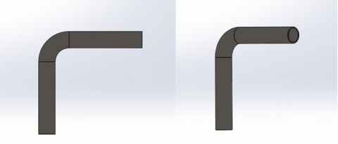
According to the standard dimensions mentioned in Table 1, the model was designed on the SolidWorks software, as shown in Figure 1 and Figure 2.
Figure 1. Pipe design in SolidWorks
Figure 2. Standard dimensions in the design (in mm)
To obtain the operational parameters of flow rate and pressure drop, and to increase accuracy in this study, AioFlo V1.09 software was used in Figure 3.
Figure 3. Calculations in AioFlo V1.09 software
3.2 Simulation of the pipe model
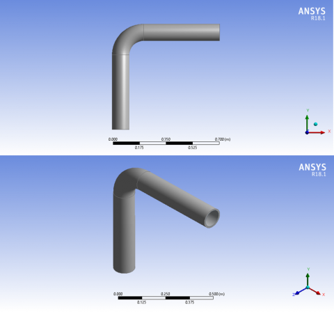
The simulation process was carried out using the Ansys program version 2018, and Figure 4 shows the geometry of the model.
Figure 4. The geometry of the model in Ansys simulation
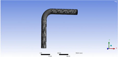
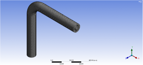
In the meshing process, Figure 5, the intention was to reduce the number of finite element models as much as possible in order to obtain the most accurate results. The numbers of nodes and elements were 651035 and 630144, respectively.
Figure 5. The meshing process
The data for the base case flow conditions of the model are listed in Table 3.
Table 3. The base case flow conditions of the model
|
Parameter |
Value |
Units |
|
Carrier fluid |
Light crude oil |
- |
|
Oil density |
834.2 |
$\left[\frac{K g}{m^3}\right]$ |
|
Oil viscosity |
0.00172 |
$[\mathrm{Pa.s}]$ |
|
Velocity |
2 |
$\left[\frac{m}{s}\right]$ |
|
Sand diameter |
200 |
$[\mu \mathrm{m}]$ |
|
Sand density |
2300 |
$\left[\frac{K g}{m^3}\right]$ |
|
Mass flow rate |
12.375 |
$\left[\frac{K g}{s}\right]$ |
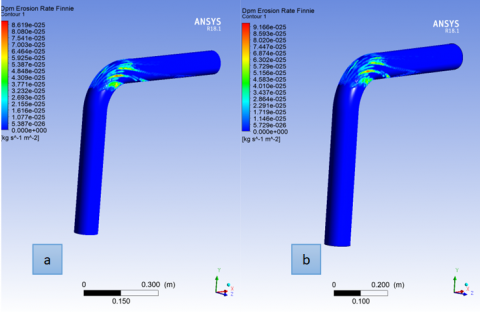
In an endeavor to comprehensively elucidate the findings, Figure 6 meticulously delineates the distribution of the Discrete Phase Model (Dpm) Erosion Rate by employing the Finnie model for each of the pipes under examination. It is imperative to underscore that the predictive nature of the Finnie model exhibits variability contingent upon the interplay of impact angle and velocity, two pivotal factors governing the erosion phenomenon.
Figure 6. Dpm erosion rate Finnie: (a) XS80S; (b) XS80
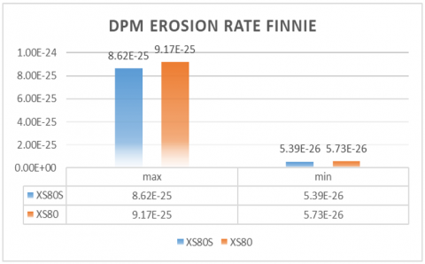
Drawing attention to Figure 7, a salient and noteworthy observation comes to the fore—namely, the discernible disparity in erosion rates between the XS80S and XS80 pipes. The evidence presented unequivocally substantiates that the erosion rate exhibited by the pipe crafted from stainless steel XS80S distinctly outperforms that of its counterpart, the XS80 steel pipe. This disparity in erosion rates resonates deeply with the core essence of the research, poised to unravel the nuanced interplay between the material composition of the pipes and the consequential erosion dynamics.
The lower erosion rate observed in the XS80S pipe when contrasted with the XS80 pipe reverberates powerfully with the overarching hypothesis that stainless steel alloys, characterized by their enhanced resistance to corrosion and mechanical robustness, would be poised to exhibit superior performance in terms of erosion resistance. Consequently, these initial findings not only affirm the research hypothesis but also lay a substantial foundation for the subsequent intricate analyses that seek to delve into the various erosion models applied and their implications within the context of pipe materials.
Figure 7. Comparison of Dpm erosion rate Finnie in the two pipes
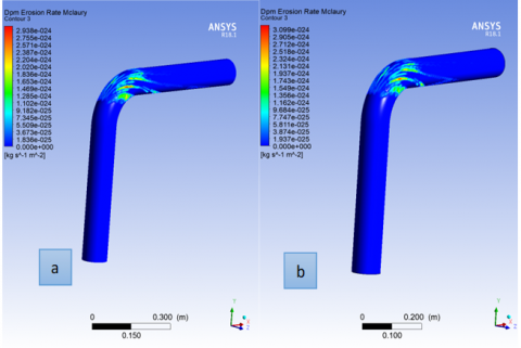
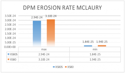
The presentation of the distribution of the Discrete Phase Model (Dpm) Erosion Rate, as per the McLaury model, is rendered manifest in Figure 8. A salient feature of this model lies in its encompassment of a constituent that forecasts the pace at which solid particles instigate the erosion process. This predictive element augments the model's efficacy in discerning the intricate interplay between particle dynamics and pipe surface degradation. Figure 9, accentuating the persisting discrepancy in erosion rates between the two types of pipes under scrutiny—XS80S and XS80. The McLaury model's predictions and the discernible erosion rate trends underscore the profound implications of material composition on erosion kinetics.
Figure 8. Dpm erosion rate McLaury: (a) XS80S; (b) XS80
Figure 9. Comparison of the Dpm erosion rate McLaury in the two pipes
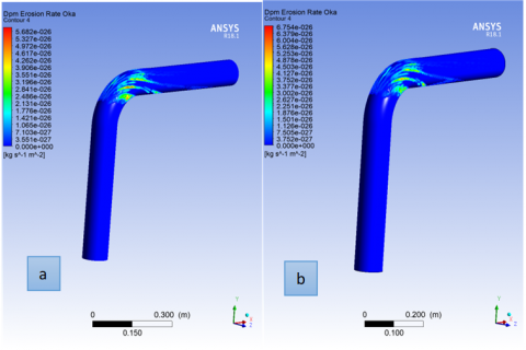
Figure 10. Dpm erosion rate Oka: (a) XS80S; (b) XS80
Figure 11. Comparison of the Dpm erosion rate Oka in the two pipes
The depiction of the Dpm erosion rate distribution based on the Oka model for each of the pipes is presented in Figure 10. The Oka model is distinctive in its incorporation of the influence exerted by the hardness of the wall material on the erosion process. This model factors in the material's hardness as a key determinant impacting the propensity for erosion. As illustrated in Figure 11, the outcomes of this analysis reaffirm a consistent trend—the erosion rate of the XS80S pipe is consistently lower than that of its XS80 counterpart.
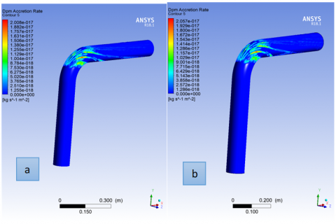
Figure 12. Dpm accretion rate: (a) XS80S; (b) XS80
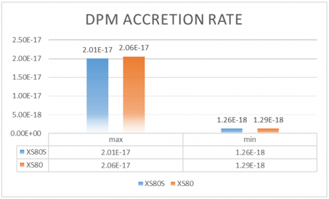
Figure 13. Comparison of the Dpm accretion rate in the two pipes
The discernible trend in erosion rates across different pipe materials substantiates the anticipated advantage of employing stainless steel, represented by XS80S, over conventional steel, represented by XS80. The incorporation of the Oka model's insights underscores the intricate relationship between material properties, specifically hardness, and their tangible effects on the susceptibility to erosion.
The DPM Accretion Rate, which quantifies the cumulative erosion over time, offers a holistic perspective on the erosion process within the pipes. This rate encapsulates the progressive accumulation of erosion-induced material loss, providing insight into the long-term durability of the pipes under scrutiny. Figure 12 presents the spatial distribution of the DPM Accretion Rate along the length of each pipe, the varying degrees of material loss across their respective surfaces.
Figure 13 offers a comparative, the distinctive erosion behaviors between the two types of pipes, XS80S and XS80. The visualization distinctly shows that the XS80S pipe consistently exhibits a lower Accretion Rate compared to its XS80 counterpart. This empirical evidence not only corroborates the earlier-established erosion rate disparities but also deepens understanding of the intricate mechanisms that govern material degradation in the context of fluid flow.
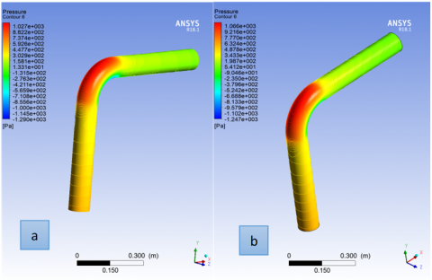
Figures 14 and 15 provide the pressure distribution and the distribution of turbulence kinetic energy along the length of the pipes, respectively. These visualizations shed light on the dynamic fluid behavior within the pipes and hold significance in elucidating the underlying fluid flow characteristics.
Figure 14. Pressure distribution along the pipe: (a) XS80S; (b) XS80
Figure 15. Turbulence kinetic energy distribution: (a) XS80S; (b) XS80
The pressure distribution, as depicted in Figure 14, showcases a prominent pattern: the highest-pressure points coincide with the bend or elbow section of the pipe. This is consistent with the anticipated hydrodynamic behavior in this configuration, where fluid experiences a constriction, leading to elevated pressure. Furthermore, as one moves away from this point of maximum pressure, a notable trend emerges: a reduction in pressure corresponds to an increase in turbulence kinetic energy. This intriguing relationship underscores the interconnected nature of pressure and turbulence in fluid dynamics.
Figure 15 introduces the distribution of turbulence kinetic energy, offering a nuanced view of how fluid energy is distributed along the pipe's length. The correlation between pressure and turbulence kinetic energy becomes evident in this depiction. As fluid experiences a pressure drop from the bend section, its kinetic energy transforms into turbulent motion, characterized by the irregular swirling of fluid particles. This visualization aligns with established fluid dynamics principles, showcasing the conversion of potential energy (pressure) into kinetic energy (turbulence).
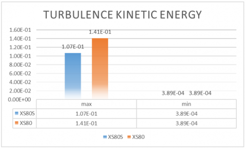
Intriguingly, Figure 16 adds another layer of understanding to the dynamic interplay between pressure and turbulence kinetics. It highlights a significant observation—the turbulence kinetic energy of the XS80S pipe is consistently lower than that of the XS80 pipe. This finding resonates with the broader trend observed in erosion and material degradation. The reduced turbulence kinetic energy within the XS80S pipe suggests a calmer fluid flow, which can contribute to minimizing the abrasive effects that could lead to erosion. Consequently, this empirical evidence adds another dimension to the benefits of employing XS80S material, as it not only demonstrates lower erosion rates but also showcases favorable flow dynamics.
Figure 16. Comparison of the turbulence kinetic energy in the two pipes
The culmination of this study's results consistently underscores a pivotal finding: The erosion rate within the stainless steel XS805 pipe is consistently lower than that observed in the steel XS80 pipe. This pronounced discrepancy can be attributed to the inherent corrosion resistance, as well as the mechanical and chemical properties characteristic of stainless steel. This distinction in erosion behavior reaffirms the vital role that material composition plays in influencing erosion dynamics.
Furthermore, the investigation into the impact of the pipe's geometry sheds light on the crucial role played by the bending area or elbow section. In this region, the erosion rate and pressure attain their zenith. The explanation lies in the generation of shear stresses within the fluid as it flows around this constricted segment. Notably, these shear stresses emerge exclusively when the fluid is in motion, absent when the fluid is stationary or experiences uniform flow velocities. This observation unveils a plausible explanation for the escalated erosion witnessed in the elbow region, elucidating the mechanics that drive the erosion process.
Importantly, the predictions derived from this study resonate harmoniously with the findings of previous researchers. In a study conducted by Xu et al. [10], similar patterns were identified, reinforcing the consistency and reliability of the current research outcomes. Moreover, the alignment extends to the observations of Sedrez and Shirazi [11], who investigated the influence of elbow orientation relative to gravity on erosion rates. Their work concurs with the present findings, suggesting that the direction of the elbow has a substantial impact on the rate of erosion. This not only corroborates the present study's insights but also substantiates the broader applicability of these conclusions across various contexts. This expanded summary provides a more in-depth perspective on the research findings and their alignment with previous studies, demonstrating a comprehensive understanding of erosion mechanisms and their broader implications.
In summary, the comprehensive analysis undertaken in this research provides a multifaceted view of erosion tendencies within the examined pipes. The comparison of erosion rates between different materials as show in Table 4, along with the exploration of geometry-induced variations, collectively contribute to the understanding of erosion mechanisms. The observed trends not only offer insights into the intricate interplay of fluid dynamics and material properties but also underscore the potential of utilizing erosion-resistant materials to enhance the durability and longevity of critical infrastructure.
Table 4. The comparison of erosion rates between different materials
|
XS80 mm3kg-1 |
XS80S mm3kg-1 |
PIPE |
||
|
MAX |
MIN |
MAX |
MIN |
Modal |
|
9.17 E-25 |
5.73E-26 |
8.62 E-25 |
5.39E-26 |
Dpm Erosion Rate Finnie |
|
3.10E-24 |
1.94E-25 |
2.94E-24 |
1.84E-25 |
Dpm Erosion Rate McLaury |
|
6.75E-26 |
3.75E-27 |
5.68E-26 |
3.55E-27 |
Dpm Erosion Rate Oka |
|
2.06E-17 |
1.29E-18 |
2.01E-17 |
1.26E-18 |
Dpm Accretion Rate |
In this study, Computational Fluid Dynamics (CFD) was employed to analyze and compare the erosion characteristics of pipes with 90° elbows fabricated from two distinct materials under the conditions of turbulent oil and sand particle transportation. The simulations enabled the prediction of erosion rate distribution and particle trajectory along the pipes, particularly through the elbow region. The study focused on the erosion characteristics of stainless-steel pipe XS80S and steel pipe XS80. The following conclusions were drawn:
i. Corrosion performance: The stainless steel XS80S pipe performed better than the steel XS80 pipe in all simulation models. The maximum Dpm Erosion Rate Finnie model for the XS80S and XS80 pipes were 8.62 E-25 mm3kg-1 and 9.17 E-25 mm3kg-1, respectively; for the McLaury model they were 2.94E-24 mm3kg-1 and 3.10E-24 mm3kg-1, respectively; for the Oka model they were 5.68E-26 mm3kg-1 and 6.75E-26 mm3kg-1, respectively. The maximum Dpm Accretion Rate for the XS80S and XS80 pipes were 2.01E-17 mm3kg-1 and 2.06E-17 mm3kg-1, respectively. The maximum Turbulence Kinetic Energy for the XS80S and XS80 pipes were 1.07E-01 and 1.41E-01, respectively.
ii. Elbow region significance: The study highlighted the elbow region as a particularly vulnerable area within pipelines. This section experienced the most severe erosion due to a confluence of pressure and turbulent kinetic energy fluctuations the precise areas that demand focused attention and protection measures. This insight enables targeted design modifications, material enhancements, and maintenance protocols that specifically address the vulnerabilities of these critical pipeline segments.
iii. Enhanced understanding of material performance: The findings of this study serve as a significant stride toward comprehending corrosion within pipelines. By meticulously comparing the erosion behaviors of two distinct materials, stainless steel XS80S and steel XS80, under varying operational conditions, we've unveiled a nuanced perspective on the interplay between material properties and erosion susceptibility. The consistent superiority of XS80S in all simulation models underscores the pivotal role of material selection in combating erosion, the durability and longevity of pipeline systems.
iv. Precise erosion prediction: By integrating Computational Fluid Dynamics (CFD), precise prediction of erosion rate distributions and particle trajectories becomes achievable. Through this advanced simulation technique, we transcend mere speculation and embark on a journey toward accurate and predictive models. This level of precision equips pipeline operators and designers with a powerful tool that aids in anticipating erosion-related challenges, facilitating proactive strategies to mitigate material loss and maintain pipeline integrity.
This study doesn't just stop at presenting results; it paves the way for future research avenues. By identifying the superior erosion resistance of stainless steel XS80S, stimulate further investigations into exploring the broader spectrum of material properties, operational conditions, and predictive models. These future endeavors hold the potential to unravel intricate corrosion mechanisms, refine erosion prediction accuracy, and contribute to the evolving body of knowledge surrounding pipeline integrity management.
Limitations of the current study may include:
·Simplified assumptions: The study relies on certain assumptions and simplifications in the CFD simulations, which may not fully capture the complexity of real-world pipeline conditions.
·Limited material selection: The study focuses on stainless steel XS80S and steel XS80, but other materials commonly used in oil pipelines should be considered for comprehensive comparisons.
·Operational variations: The study analyzes erosion under specific operational conditions. Further investigations should explore a wider range of flow rates, sand concentrations, and fluid properties to account for variations typically encountered in oil pipeline operations.
The in-depth understanding of corrosion behavior gleaned from this study empowers decision-makers in the pipeline industry to make informed choices. Whether it's selecting appropriate materials for pipeline construction, devising effective maintenance schedules, or implementing erosion mitigation strategies, the insights garnered here bolster the ability to make decisions grounded in empirical evidence and scientific rigor.
In summation, the results of this study enrich the comprehension of corrosion in pipeline systems by unraveling the multifaceted relationship between material properties, fluid dynamics, and erosion susceptibility. The findings underscore the importance of material selection, targeted design modifications, and maintenance protocols in managing erosion and maintaining pipeline integrity. Future research should delve into refining predictive models, investigating corrosion mechanisms, and exploring a wider range of materials and operational conditions. This comprehensive understanding transcends theoretical speculation and equips stakeholders with actionable insights that foster pipeline longevity, operational efficiency, and industry-wide advancements in corrosion management.
Authors would like to thank University of Technology-Iraq for supporting the present work.
[1] Gong, K., Wu, M., Liu, G. (2020). Stress corrosion cracking behavior of rusted X100 steel under the combined action of Cl− and HSO3− in a wet–dry cycle environment. Corrosion Science, 165: 108382. https://doi.org/10.1016/j.corsci.2019.108382
[2] Sun, D., Wu, M., Xie, F. (2018). Effect of sulfate-reducing bacteria and cathodic potential on stress corrosion cracking of X70 steel in sea-mud simulated solution. Materials Science and Engineering: A, 721: 135-144. https://doi.org/10.1016/j.msea.2018.02.007
[3] Orasheva, J. (2017). The effect of corrosion defects on the failure of oil and gas transmission pipelines: A finite element modeling study. Master’s Thesis, University of North Florida, College of Computing, Engineering, and Construction. https://digitalcommons.unf.edu/etd/763.
[4] Popoola, L.T., Grema, A.S., Latinwo, G.K., Gutti, B., Balogun, A.S. (2013). Corrosion problems during oil and gas production and its mitigation. International Journal of Industrial Chemistry, 4: 1-15. https://doi.org/10.1186/2228-5547-4-35
[5] Hadžiahmetović, H., Hodžić, N., Kahrimanović, D., Džaferović, E. (2014). Computational Fluid Dynamics (CFD) based erosion prediction model in elbows. Technical Gazette, 3651: 275-282.
[6] Zeng, L., Zhang, G.A., Guo, X.P. (2014). Erosion–corrosion at different locations of X65 carbon steel elbow. Corrosion Science, 85: 318-330. https://doi.org/10.1016/j.corsci.2014.04.045
[7] Adedeji, O.E., Duarte, C.A.R. (2020). Prediction of thickness loss in a standard 90 elbow using erosion-coupled dynamic mesh. Wear, 460: 203400. https://doi.org/10.1016/j.wear.2020.203400
[8] Duarte, C.A.R., de Souza, F.J. (2021). Dynamic mesh approaches for eroded shape predictions. Wear, 484: 203438. https://doi.org/10.1016/j.wear.2020.203438
[9] Zhang, J., Zhang, H., Chen, X., Yu, C. (2021). Gas–solid erosion wear characteristics of elbow pipe with corrosion defects. Journal of Pressure Vessel Technology, 143(5): 051501. https://doi.org/10.1115/1.4050315
[10] Xu, L., Wu, F., Yan, Y., Ma, X., Hui, Z., Wei, L. (2021). Numerical simulation of air-solid erosion in elbow with novel arc-shaped diversion erosion-inhibiting plate structure. Powder Technology, 393: 670-680. https://doi.org/10.1016/j.powtec.2021.08.022
[11] Sedrez, T.A., Shirazi, S.A. (2021). Erosion evaluation of elbows in series with different configurations. Wear, 476: 203683. https://doi.org/10.1016/j.wear.2021.203683
[12] Brown, G.O. (2002). The history of the Darcy-Weisbach equation for pipe flow resistance. In Environmental and Water Resources History, pp. 34-43. https://doi.org/10.1061/40650(2003)4
[13] Oka, Y.I., Okamura, K., Yoshida, T. (2005). Practical estimation of erosion damage caused by solid particle impact: Part 1: Effects of impact parameters on a predictive equation. Wear, 259(1-6): 95-101. https://doi.org/10.1016/j.wear.2005.01.039
[14] Oka, Y.I., Yoshida, T. (2005). Practical estimation of erosion damage caused by solid particle impact: Part 2: Mechanical properties of materials directly associated with erosion damage. Wear, 259(1-6): 102-109. https://doi.org/10.1016/j.wear.2005.01.040
[15] Al-Baghdadi, M.A., Resan, K.K, Al-Waily, M. (2017). CFD investigation of the erosion severity in 3D flow elbow during crude oil contaminated sand transportation. Engineering and Technology Journal, 35(9): 930-935. https://doi.org/10.30684/etj.35.9A.10
[16] ASME/ANSI B36.19 Standard for Stainless Steel Pipe, New York: ANSI/ ASME, 2016. https://doi.org/10.1115/PVP2016-63614
[17] Rice, D.A., Waterland, J., Chandler, D.G. (2016). Estimation of head loss due to flow intrusion with inner ring spiral wound gaskets. In Pressure Vessels and Piping Conference, 50381: V002T02A011. https://doi.org/10.1115/PVP2016-63614
[18] Furkan Sokmen, K., Bedrettin Karatas, O. (2020). Investigation of air flow characteristics in air intake hoses using CFD and experimental analysis based on deformation of rubber hose geometry. Journal of Applied Fluid Mechanics, 13(3): 871-880. https://doi.org/10.29252/JAFM.13.03.30497
[19] Zhang, J., McLaury, B.S., Shirazi, S.A. (2018). Application and experimental validation of a CFD based erosion prediction procedure for jet impingement geometry. Wear, 394: 11-19. https://doi.org/10.1016/j.wear.2017.10.001
[20] Xie, Z., Cao, X., Zhang, J., Darihaki, F., Karimi, S., Xiong, N., Li, Q. (2021). Effect of cell size on erosion representation and recommended practices in CFD. Powder Technology, 389: 522-535. https://doi.org/10.1016/j.powtec.2021.05.066