Samuel Vega-Zuñiga*![]() | Juan Gabriel Rueda-Bayona
| Juan Gabriel Rueda-Bayona![]() | Adalberto Ospino-Castro
| Adalberto Ospino-Castro![]()
© 2024 The authors. This article is published by IIETA and is licensed under the CC BY 4.0 license (http://creativecommons.org/licenses/by/4.0/).
OPEN ACCESS
The traditional assessment of wind resource considers the ambient factors like temperature, pressure and humidity as a secondary parameter, and focus on the statistically evaluation of wind magnitude and direction. Nevertheless, the evaluation requires a deeper analysis of the above ambient factors, because they are thermodynamically linked, and the energy flux among them will affect the wind dynamics. This research aims to analyse the interactions of temperature, pressure, and humidity variables with the wind speed with an inverse approach, it means that wind will be controlled by the ambient variables. We conducted a statistical analysis using data from a meteorological station located in the University of the Coast in Barranquilla, Colombia. The methodology is based on a Design of Experiments-Analysis of Variance (DOE-ANOVA) with a 32 factorial design. The estimated effects from the DOE-ANOVA results were utilized to generate standardized effect equations, for evaluating the response of wind speed during changes of the studied ambient variables (factors). The results evidenced that the applied methodology provided information about the non-linear interactions of the analysed variables, and the standardized effect equations were tested against a liner regression model with satisfactory results.
Design of Experiments-Analysis of Variance, wind speed, temperature, pressure, humidity, multiple regression
The rapid growth of humanity in all its dimensions can be translated into a greater demand for fossil fuels, which urgently need to be replaced by environmentally friendly energy sources. Energy transition is a necessary step to ensure the well-being of our planet. Wind energy is playing a crucial role in global energy growth as it is clean and free from pollution [1].
In this sense, wind energy is one of the most exploited energies resources, currently being the most efficient among all renewable energies [2]. Having a proper understanding of the behaviour of the various atmospheric variables that influence the wind speed plays a crucial role in the comprehension of wind energy. Also, evaluating the behaviour of the different atmospheric variables that drives the wind speed performance, plays a preponderant role for an efficient use of wind energy [3].
Several statistical methods are applied for assessing the wind resource, and the use of the Design of Experiments- Analysis of Variane (DOE-ANOVA) is little documented. DOE-ANOVA is a methodology that allows the development of a response variable model through the iteration of other input variables. Some authors have defined DOE as a set of methods used to develop a process aimed at obtaining information, which is then analysed using Analysis of Variance (ANOVA) [4]. A precise explanation of DOE is addressed by Trnka et al. [5], where the author explains how through these types of designs, the number of experiments can be minimized. Also, the method has shown versatility in the academic and industrial fields. For example, the DOE-ANOVA applications can be seen in Gurba-Bryśkiewicz et al. [6]’s study, where is utilized like a strategy to optimize the composition and production of RNA-LNPs (lipid nanoparticles). Additionally, Adewumi and Azeez [7] presented a study focused on optimizing the production of biofuels from citrus peels using DOE as a technique. The research explains the response variables through the iteration of the independent variables. From Costa and Barros Bagno [8]’s study, it is noticed the used of ANOVA and its worldwide use like statistical method. Similarly, Elbanna et al. [9] mentioned that DOE ANOVA is a flexible methodology because allows to evaluate the response of a variable with different intervals within a defined limit range, hence, the behaviour of the evaluated parameter can be explained through the responses generated by the effects and interactions of the factors.
The use of factorial DOE-ANOVA analysis has been reported in several studies of Oceanography and Ocean Engineering such as wave run-up, debris loads, coastal protection, naval design, and ocean modelling [10-13]. Tahavorgar and Quaicoe [14] presented an example of a design of experiments that models the wind speed in wind turbine units is presented. Ukita et al. [15] explained how a factorial design works and how each input variable affects the response variables. In Lee et al. [16]’s study, a DOE-ANOVA is used to validate the researcher’s suggested method, demonstrating the versatility of the methodology. Zedan et al. Zedan et al. [17] explained how to construct an experimental design that studies the interaction of different variables considered in the study through the development of a regression model. Subsequently, an ANOVA is conducted to validate the fit and relevance of the model under the recreated conditions.
According to the literature review, it was observed that there is not available studies about the use of wind speed, ambient pressure, humidity and temperature time series to perform a DOE-ANOVA factorial design for analysing non-linear interactions. Here in, this research proposes the use of a DOE-ANOVA to analyse the response of wind speed when the ambient parameters change. In this context, the proposed method analyses the effects as input variables (temperature, pressure, and humidity) and the cause (i.e., wind) as the output or response variable. As a result, the methodology offers an inverse approach the evaluate the wind performance based on the effect of the ambient variables.
To analyse the effect of atmospheric variables i.e. pressure, temperature and humidity, on the response of wind speed, the following methodological process was developed:
1. START
2. DEFINE The input and response variables of the model.
3. DATA PREPARATION of the experiment (DOE) -ANOVA conducted through the Statgraphics software.
4. DESIGN OF THE EXPERIMENT
5. ANALYSIS of the DOE-ANOVA results through standardized Pareto diagrams and main effect diagrams.
6. CONFIGURE AND TUNE model.
7. OPTIMIZE model parameters for best performance.
8. COMPARE ANOVA vs multiple regression model.
9. ESTABLISH parameterized equations according to the statistical results.
10. END
Table 1. Experimental factors for wind speed
|
Symbol |
Factor |
Units |
Low |
High |
Levels |
|
A |
Humidity |
% |
0 |
98 |
10 10 |
|
B |
Pressure |
mmHg |
753.1 |
761.3 |
|
|
C |
Temperature |
℃ |
0 |
34.8 |
10 |
A database obtained from the meteorological station at the University of the Coast was used to provide the measured input data. The dataset has one year of surface meteorological variables (10 m) with 5-minute intervals: wind speed, temperature, humidity, and atmospheric pressure. A 32 factorial design without replicates was configured, were temperature, humidity, and atmospheric pressure are the factors and the minimum and maximum levels were set according the statistical results of each factor (Table 1). The multivariate analysis was performed through the Statgraphics Centurion XVI statistical software. This software offers a user-friendly interface with high-quality graphics and easily interpretable data presentation. Additionally, it allows various data processing operations, enhancing versatility when comparing ANOVA with regression analysis. Analysis of Variance (ANOVA), Pareto chart, and response surface diagram were conducted by means of the software.
An experiment is a research process that generate information through a structured process as DOE method does. The application of methods such as the Design of Experiments (DOE), as elucidated by Elbanna et al. [9], provides a systematic framework for understanding the effects of various factors, considered as independent variables, on a given response or dependent variable, in that sense, DOE methodology, offers a structured approach to experimentation. It involves carefully planning and executing a set of experimental runs to systematically vary the independent variables and observe their impact on the response. This method enables the identification of key factors influencing the response, providing a deeper understanding of the system under investigation.
Importantly, the DOE process is a precursor to the Analysis of Variance (ANOVA) analysis, a statistical technique detailed by Rueda-Bayona et al. [10]. Before delving into ANOVA, the DOE methodology is applied to design an experiment that systematically explores the parameter space. This systematic exploration aids in the identification of significant factors and their potential interactions, the DOE-ANOVA method, as explained by Rueda-Bayona et al. [10], delves into the intricate relationships between the response variable and the identified factors. It not only assesses the main effects of each factor but also explores the interactions among them. This nuanced understanding is crucial for comprehensively unravelling the dynamics of the system and discerning the unique contributions of each variable [18-20].
Upon the meticulous analysis of the results obtained from the Design of Experiments (DOE), the study progressed to the application of the Response Surface Method (RSM), as detailed by Fragasso et al. [11]. The RSM method proves instrumental in identifying optimal operational conditions that maximize the wind speed response. This method takes into account all main factors and their interactions, providing a comprehensive exploration of the parameter space. The multilevel factorial design comprises 1000 experiments, strategically executed in a randomized single block to mitigate any potential systematic bias. Table 1 succinctly outlines the factors under consideration and their respective levels. The strategic integration of the DOE and RSM methodologies enhances the depth of the study, facilitating the identification of optimal conditions that significantly influence wind speed. The deliberate use of a multilevel factorial design and randomized execution further ensures the robustness and reliability of the derived insights.
The model evaluates the variables and their levels, the results are adjusted to a second-degree multivariable polynomial (1) that is described by GilPavas et al. [21].
$y_i=\beta_0+\sum_{i=1}^3 \beta_i X_i+\sum_{i=1}^3 \beta_{i i} X_{i i}^2+\sum_{i=1}^3 \sum_{i=1}^3 \beta_{i j} X_i X_j$ (1)
where, yi is the response variable (dependent variable), β0, βi, βii & βij are the regression coefficients for the intercept and Xi, Xj represent the independent variables. The Eq. (1) can be used to make predictions of the process and for optimization. Rueda-Bayona et al. presented [19] the calculation of the variable to be predicted through the ANOVA standardized effects represented in the Eq. (2):
$y=\mu+\frac{\alpha_i}{2} \cdot \hat{X}_i+\frac{\beta_j}{2} \cdot \hat{X}_i+\frac{\delta_{i j}}{2} \cdot \hat{X}_i$ (2)
where, y is the dependent variable, μ is the mean of dependent variable, αi are the first-order effects, βi are second-order effects, δi are the iterations between effects, and $\hat{X}_i$ is the normalized factor. The $\hat{X}_i$ is calculated through Eq. (3), taken from Blanco León [22]’s study, where x is the independent variable and a, b are the normalized limits -1 y 1 respectively.
$\hat{X}_i=a+\frac{[x-\min (x)] \cdot(b-a)}{\max (x)-\min (x)}$ (3)
In this section we present the results of the DOE-ANOVA, and the standardized effects model and multiple linear regression model as well. The effects of factors on wind speed are retrieved from the DOE-ANOVA (Figure 1).
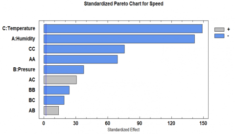
Figure 1. Standardized Pareto chart for wind speed
In Figure 1, the standardized Pareto chart for wind speed visually represents the significant influence of various factors on the response variable. It is noteworthy that both temperature and pressure demonstrated an inverse correlation with wind speed, that is, the higher atmospheric pressure and air temperature coincide with lower wind speeds. In line with this, elevated humidity levels are associated with decreased wind speed. The figure also shows a positive effect of humidity-temperature and humidity-pressure on the wind speed, while pressure-temperature exhibits an inverse relationship.
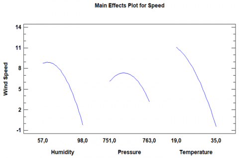
In Figure 2, the main effects plot provides a comprehensive visualization of the impacts of varying humidity, pressure and temperature on the system. The plot reveals a positive effect on humidity within the range of 0% to approximately 60%, followed by a subsequent negative effect as humidity approaches 98%. In the case of pressure, the effect is subtly positive initially and the transition to a slightly negative influence. Noteworthy is the marked negative effect of temperature, a trend consistent with the data observed in the Pareto diagram. These nuanced patterns underscore the intricate relationships among these variables, shedding light on their individual contributions to the system’s behaviour. The alignment between the main effects plot and the Pareto diagram further validates the robustness and consistency of the observed effects.
The aforementioned results of Figures 1-2 are considered proper when analysing the physics of the problem. When wind blows produce a stress over the study area, provoking momentum and energy transfer. The wind stress eases the thermal transfer energy in the surface atmospheric system, because the mechanical transport effect of wind changes the mass and heat balance. In the variable terms, when wind surface rises, the water vapor is dragged and the air humidity, temperature and pressure decreases. In the opposite, when wind speed reduces, a local increment of water vapor due to the solar radiation occurs, what provokes a rise in the temperature, humidity and ambient pressure.
Figure 2. Main effects plot for wind speed
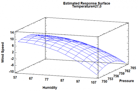
Figure 3. Response surface plot for wind speed
Figure 3 illustrates the estimated temperature response surface at 27.0℃, revealing a noticeable curvature that indicate the data conform to a second order model. The highest achievable speed corresponds to a specific parameters value explained by the pattern observed in previous presented figure namely, a humidity level close to 60% and a pressure around 759 mmHg. Evaluating the impact of factors on the response variable involve analysing results the design of experiments (DOE) through Pareto charts and the main effects chart in the context of the analysis of variance (ANOVA). These visualizations provide a comprehensive understanding of how the considered factors influence the system, enhancing the interpretability of the observed relationships.
Table 2 presents the estimates for individual effects and interactions, accompanied by their respective standard errors. the standard error quantifies the sampling error associated with each effect, providing a measure of the precisions of the estimates, the ANOVA standardized effects model was written:
$\begin{aligned} \text { Wind speed }(m / s)= & 7,16311+\frac{-8,99883}{2} \cdot \hat{X}_A+\frac{-1,27341}{2} \cdot \hat{X}_B+\frac{-15,04161}{2} \cdot \hat{X}_C+\frac{-33,1153}{2} \cdot \hat{X}_A{ }^2+\frac{3,47771}{2} \cdot \hat{X}_A \hat{X}_B+ \\ & \frac{315,2632}{2} \cdot \hat{X}_A \hat{X}_C+\frac{-2,35309}{2} \cdot \hat{X}_B{ }^2+\frac{-5,41997}{2} \cdot \hat{X}_B \hat{X}_C+\frac{-17,3619}{2} \cdot \hat{X}_C{ }^2\end{aligned}$ (4)
Table 2. Estimated effects of DOE ANOVA factorial design
|
Estimated Effects for Speed (m/s) |
|||
|
Effect |
Estimate |
Error Estd. |
V.I.F. |
|
Average |
7.6311 |
0.0159035 |
|
|
A: Humidity |
-8.99883 |
0.0635189 |
6.20284 |
|
B: Pressure |
-2.94355 |
0.0786011 |
1.61886 |
|
C: Temperature |
-11.5207 |
0.0772618 |
6.13779 |
|
AA |
-5.79621 |
0.0837993 |
84.5024 |
|
AB |
2.12921 |
0.154477 |
1.63225 |
|
AC |
2.93592 |
0.0955158 |
88.7514 |
|
BB |
-5.03933 |
0.211863 |
1.3447 |
|
BC |
-3.64674 |
0.19141 |
1.32862 |
|
CC |
-3.67011 |
0.0484409 |
19.1494 |
Note: Standard errors based on the total error with 61886 Df.
Table 3. Statistical parameters of the DOE ANOVA factorial design
|
Coef. Regression for Speed |
|
|
Coefficient |
Estimate |
|
constant |
-40191.0 |
|
A: Humidity |
-5.94434 |
|
B: Pressure |
106.075 |
|
C: Temperature |
28.8907 |
|
AA |
-0.00689615 |
|
AB |
0.00865533 |
|
AC |
0.00895099 |
|
BB |
-0.0699907 |
|
BC |
-0.0379869 |
|
CC |
-0.0286727 |
Using a linear regression analysis, the formulation of the equation representing the response variable is based on the regression coefficients derived from the DOE ANOVA factorial as detailed in Table 3 where the values of the variables are specificized in their original units, the results equation takes the form:
$\begin{aligned} \text { ind speed }= & -40191,0-5,94434 * X_A+106,075 * X_B+28,8907 * X_C-0,00689615 * X_A^2+0,00865533 * X_A * \\ & X_B+0,00895099 * X_A * X_C-0,0699907 * X_B^2-0,0379869 * X_B * X_C-0,0286727 * X_C^2\end{aligned}$ (5)
Table 4. ANOVA table of DOE ANOVA factorial design
|
Analysis of Variance for Speed |
|||||
|
Source |
Sum of Squares |
Df |
Middle Square |
f-ratio |
P-value |
|
Model |
15786.0 |
3 |
5262.01 |
1162.90 |
0.0000 |
|
Residual |
280056 |
61892 |
4.52492 |
|
|
|
Total (corr.) |
295842 |
61895 |
|
|
|
Table 4 reveals that all the effects have a P-value lower than 0.05, pointing their significant deviation from zero with a 95% of confidence level. This attests to the statistical significance of the factors influencing wind speed behaviour. This table also shows that the R2 and the adjusted R2 statistic explains 46.59%, and 46,58% of the variability, respectively. These metrics underscore the model’s capability to account for nearly half of the observed variations in wind speed.
Following the DOE ANOVA results, a multi-response optimization is conducted, aiming for an attainment of 6.7, as depicted in (Table 5). This optimization process seeks to identify optimal conditions that yield the desired outcome and further enhance the practical utility of the conducted experiments.
Table 5. Multiple response optimization of the DOE ANOVA factorial design
|
|
Desirability |
|
Weight |
Weight |
|
|
|
Response |
Low |
High |
Goal |
First |
Second |
Impact |
|
Speed |
0.0 |
13.4 |
6.7 |
1.0 |
1.0 |
3.0 |
Table 6. Desirability optimization of DOE ANOVA factorial design
|
Factor |
Low |
High |
Optimum |
|
Humidity |
57 |
98.0 |
78.2613 |
|
pressure |
751.0 |
763.0 |
756.94 |
|
Temperature |
19 |
35.0 |
27.4234 |
Tables 5-6 delineate the optimal combination of factors for optimizing the wind speed, maintaining a desirability of 6.7. Specifically, Table 6 provides a comprehensive view of high, low and optimal values, emphasizing the key parameters to contribute to the desired wind speed. These findings serve as a roadmap for configuring the factors optimally, aligning with the pursuit of achieving optimal performance in the system.
Table 7. Path of maximum ascent for speed
|
Humidity |
Pressure |
Temperature |
Prediction for Speed |
|
(%) |
(mmHg) |
(℃) |
(m/s) |
|
77.5 |
757.0 |
27.0 |
7.16311 |
|
78.5 |
757.099 |
27.498 |
6.54962 |
|
79.5 |
757.202 |
27.9932 |
5.91424 |
|
80.5 |
757.312 |
28.4858 |
5.25661 |
|
81.5 |
757.426 |
28.9761 |
4.57633 |
|
82.5 |
757.545 |
29.4644 |
3.87302 |
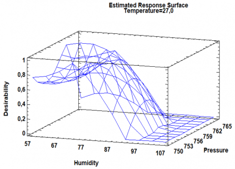
Figure 4. Response surface plot for desirability
Table 7 displays the trajectory of maximum ascent, originating from the center of the current experimental region, this includes the desirability value factors and response variable. It illustrated the path along which the estimate response exhibits the most rapid change with minor adjustments in the experimental factors. This representation is crucial for identifying optimal conditions when conducting additional experiments, especially with the goal of increasing the speed.
Table 7 shows 6 data points have been generated by systematically varying humidity in 1.0% increments.
Figure 4 depicts the achieved desirability at its optimal value (1), indicative of a specific combination of humidity, pressure and temperature. This optimal condition represents an ideal state, maximizing the desirable outcomes according to the defined criteria. The figure provides a visual representation of the convergence towards the optimum, offering insights into the synergistic effects of the considered variables on achieving the system performance.
3.1 Multiple regression
The multiple regression analysis section plays a pivotal role in this study, providing a robust analytical framework to comprehend the intricate relationship between multiple independent variables and the response variable. Multiple regressions allow modelling and quantifying the joint influences of diverse variables, offering a powerful tool to explore patterns, identify trends, and predict outcomes. In this context, a multiple regression was constructed to analyse wind speed, incorporating three independent variables (factors) temperature, pressure and humidity. The formulation of the regression equation as represented in Eq. (6):
Wind speed $=228,077-0,0285903 *$ Humidity $-0,296461 *$ Pressure $+0,109862 *$ Temperature (6)
This equation provides a quantitative representation of the relationships between the variables, revealing the impact of humidity, pressure, and temperature on wind speed. Notably, the coefficients, presented in the equation, are accompanied by a 95% confidence interval, a measure of the precision and reliability of the estimates. The incorporation of this confidence interval enhances the robustness of the regression model, instilling confidence in the accuracy of the identified relationships. These findings contribute to a more nuanced understanding of the factors influencing wind speed, backed by a rigorous statistical framework.
Table 8. Analysis of variance multiple regression variance analysis
|
Source |
Sum of Squares |
Df |
Middle Square |
f-ratio |
P-value |
|
A: Humidity |
1234.78 |
1 |
1234.78 |
483.65 |
0.0000 |
|
B: Pressure |
96.6441 |
1 |
96.6441 |
37.85 |
0.0000 |
|
C: Temperature |
4217.45 |
1 |
4217.45 |
1651.94 |
0.0000 |
|
AA |
12214.2 |
1 |
12214.2 |
4784.19 |
0.0000 |
|
AB |
485.028 |
1 |
485.028 |
189.98 |
0.0000 |
|
AC |
2412.09 |
1 |
2412.09 |
944.80 |
0.0000 |
|
BB |
1444.41 |
1 |
1444.41 |
565.76 |
0.0000 |
|
BC |
926.694 |
1 |
926.694 |
362.98 |
0.0000 |
|
CC |
14655.1 |
1 |
14655.1 |
5740.30 |
0.0000 |
|
Total error |
157997 |
61886 |
2.55303 |
|
|
|
Total (corr.) |
295842 |
61895 |
|
|
|
Table 8 displays critical metrics for evaluating the efficacy and robustness of the regression model. The R2 coefficient, indicates the fraction of variance in the dependent variable explained by the model, reaches 5.34%. Simultaneously, the adjusted R2, tailored for models with varying independent variables, stands at 5.33%. The use of adjusted R2 is particularly pertinent when contrasting models of variable complexity. The proximity between these two values suggests that the inclusion of all variables is justified, with no need to exclude any factors from the model.
Delving into the specifics, the R2 statistic indicates that the adjusted model explains 5.34% of the variance, while the adjusted R2 refines this figure to 5.33%. This consistency reinforces the model's robustness, supporting the decision to retain all variables.
Regarding to the individual predictors, the statistical significance of 'speed' is evident, as reflected in a p-value less than 0.05. This low p-value provides compelling evidence to assert a statistically significant relationship between 'speed' and predictor variables. In practical terms, this implies that alterations in predictor variables significantly impact speed, with a probability of less than 5% for this relationship to be random, establishing a confidence level of 95%. The consistency of these findings underscores the reliability of the model's predictions, emphasizing the crucial importance of predictor variables in explaining variations in speed.
In summary, the meticulous analysis of the regression model, considering both overall fit and individual predictor significance, confirms the validity and robustness of the model's predictions. The inclusion of all variables is supported, providing valuable insights into the fundamental influence of these predictors on speed variations.
The study used wind speed data from a local meteorological station in Barranquilla (Colombia) with five-minute intervals over the course of one year, demonstrated that the response variable, namely Wind Speed, to perform a DOE-ANOVA analysis. The results showed that wind speed can be explained by the effects of Temperature, Humidity, and ambient Pressure. This means that DOE-ANOVA is a tool that enable the recreation of experimental scenarios capable of explaining the behaviour and interaction of variables while maximizing efficiency and seeking reliable conclusions.
It was evident that wind speed is directly and indirectly influenced by the input variables considered in the experiment: temperature, pressure, and humidity. This study evaluated the capability of modelling the wind speed through two statistical models: a standardized effect model written with the DOE-ANOVA results and a linear regression model. Both models explained the data behaviour, however, as seen in the results, the standardized effect model worked better.
The DOE ANOVA 23 factorial design allowed to identify the non-linear effects of the ambient parameters on the wind speed, and provided statistical parameters to set a parameterized equation to model the wind speed. The comparison between the standardized effect model and the linear regression model showed that the first outperformed.
Finally, this research not only evidence that DOE-ANOVA ease the understanding of non-linear interactions among variables, but also, evidenced that the use of estimated effects to generate a standardized effect model is an alternative to estimate the response of wind speed varying the magnitude of temperature, pressure and humidity within local value ranges.
[1] Santhosh, M., Venkaiah, C., Vinod Kumar, D.M. (2020). Current advances and approaches in wind speed and wind power forecasting for improved renewable energy integration: A review. Engineering Reports, 2(6): e12178. https://doi.org/10.1002/eng2.12178.
[2] Tapia, C. (2023). Las principales energías renovables según Mark Jacobson. laverdadnoticias.com, Cancún.
[3] Lee, C.H., Chou, C.C., Chung, X.H., Zeng, P.W. (2016). Applying climate big-data to analysis of the correlation between regional wind speed and wind energy generation. In 2016 3rd International Conference on Green Technology and Sustainable Development (GTSD), Kaohsiung, Taiwan, pp. 173-177. https://doi.org/10.1109/GTSD.2016.49
[4] Garza Villegas, J. (2013). Experiment design application for analysis of the drying a product. Innovaciones de Negocios (19): 145-158.
[5] Tůmová, O., Kupka, L., Netolický, P. (2018). Design of experiments approach and its application in the evaluation of experiments. In 2018 International Conference on Diagnostics in Electrical Engineering (Diagnostika), Pilsen, Czech Republic, pp. 1-4, https://doi.org/10.1109/DIAGNOSTIKA.2018.8526104
[6] Gurba-Bryśkiewicz, L., Maruszak, W., Smuga, D.A., Dubiel, K., Wieczorek, M. (2023). Quality by design (QbD) and design of experiments (DOE) as a strategy for tuning lipid nanoparticle formulations for RNA delivery. Biomedicines, 11(10): 2752. https://doi.org/10.3390/biomedicines11102752
[7] Adewumi, I.O., Azeez, A.A. (2023). Optimization of biofuel production process using design of experiments (Doe). Petro Chem Indus Intern, 6(2): 75-85. https://www.researchgate.net/publication/370132014.
[8] Costa, M., Barros Bagno, R. (2016). Aplicação das técnicas ANOVA e DOE na solução de problemas complexos de manufatura: Estudo em uma fábrica de motores a diesel. https://www.researchgate.net/publication/303603669.
[9] Elbanna, N., Nofal, A., Hussein, A., Tash, M.M. (2020). Mechanical properties of thin wall ductile iron: Experimental correlation using ANOVA and DOE. Key Engineering Materials, 835: 171-177. https://doi.org/10.4028/www.scientific.net/KEM.835.171
[10] Rueda-Bayona, J.G., Guzmán, A., Cabello Eras, J.J. (2020). Selection of JONSWAP spectra parameters during water-depth and sea-state transitions. Journal of Waterway, Port, Coastal, and Ocean Engineering, 146(6): 04020038. https://doi.org/10.1061/(asce)ww.1943-5460.0000601
[11] Fragasso, J., Moro, L., Lye, L.M., Quinton, B.W. (2019). Characterization of resilient mounts for marine diesel engines: Prediction of static response via nonlinear analysis and response surface methodology. Ocean Engineering, 171: 14-24. https://doi.org/10.1016/j.oceaneng.2018.10.051
[12] Young, D.L., Scully, B.M. (2018). Assessing structure sheltering via statistical analysis of AIS data. Journal of Waterway, Port, Coastal, and Ocean Engineering, 144(3): 04018002. https://doi.org/10.1061/(ASCE)WW.1943-5460.0000445
[13] Rueda-Bayona, J.G., Carrillo, J., Cabello Eras, J.J. (2023). The wind-current-water levels effect over surface wave parameters nearby the Magdalena River delta: A numerical approach. Mathematical Modelling of Engineering Problems, 10(3): 993-1002. https://doi.org/10.18280/mmep.100333
[14] Tahavorgar, A., Quaicoe, J.E. (2013). Estimation of wake effect in wind farms using design of experiment methodology. In 2013 IEEE Energy Conversion Congress and Exposition, Denver, CO, USA, pp. 3317-3324. https://doi.org/10.1109/ECCE.2013.6647136
[15] Ukita, Y., Matsushima, T., Hirasawa, S. (2012). A note on ANOVA in an experimental design model based on an orthonormal system. In Proceedings 2012 IEEE International Conference on Systems, Man, and Cybernetics, SMC 2012, Seoul, Republic of Korea, pp. 1990-1995. https://doi.org/10.1109/ICSMC.2012.6378030
[16] Lee, D., Ahn, J., Oh, S.Y. (2014). Response surface smoothing for wind tunnel testing based on design of experiment with subspace partitioning. In 2014 14th International Conference on Control, Automation and Systems (ICCAS 2014), Gyeonggi-do, Korea (South), pp. 207-211. https://doi.org/10.1109/ICCAS.2014.6987987
[17] Zedan, Y., Songmene, V., Samuel, A.M., Samuel, F.H., Doty, H.W. (2022). Assessment of the influence of additives on the mechanical properties and machinability of Al-11% Si cast alloys: Application of DOE and ANOVA methods. Materials, 15(9): 3297. https://doi.org/10.3390/ma15093297
[18] Rueda-Bayona, J.G., Guzmán, A., Osorio, A.F. (2022). DOE-ANOVA for identifying the effect of extreme sea-states over the structural dynamic parameters of a floating structure. Mathematical Modelling of Engineering Problems, 9(3): 839-848. https://doi.org/10.18280/mmep.090334
[19] Rueda-Bayona, J.G., Paez, N., Cabello Eras, J.J., Sagastume Gutierrez, A. (2022). DOE-ANOVA to optimize hydrokinetic turbines for low velocity conditions. Mathematical Modelling of Engineering Problems, 9(4): 979-988. https://doi.org/10.18280/mmep.090415
[20] Montgomery, D.C. (2003). Diseño y Análisis de Experimentos. Limusa Wiley.
[21] GilPavas, E., Medina, J., Dobrosz-Gómez, I., Gómez, M.Á. (2016). Degradación de colorante amarillo 12 de aguas residuales industriales utilizando hierro cero valente, peróxido de hidrógeno y radiación ultravioleta. Información Tecnológica, 27(3): 23-34. https://doi.org/10.4067/S0718-07642016000300004
[22] Blanco León, J.D. (2021). Potencial de energía solar offshore en la región del caribe Colombiano. Universidad Militar Nueva Granada, Bogotá.