Ali Jalal Ali*![]() | Ali Fahem Abbas
| Ali Fahem Abbas![]() | Mohamed Ahmed Abdelhakem
| Mohamed Ahmed Abdelhakem![]()
© 2024 The authors. This article is published by IIETA and is licensed under the CC BY 4.0 license (http://creativecommons.org/licenses/by/4.0/).
OPEN ACCESS
This study deals with ordinary differential equations and their solutions consuming effective numerical methods. We observing for more accurate numerical methods proximate to MATLAB solutions. Approaches are Adams-Bashforth and Rung-Kutta-4 ought very good solutions, in the first response with ordinary differential equations of the primary order. Similarly, evaluation of modified second order numerical answers using, MATLAB and Adams-Bashfort-Moulton, by differential equation addition to numerical modeling methods expending fourth-order Runge-Kutta yielded excellent results. For the reason that the solutions are validated with high credibility, we explored in turn to best approximation results computed for the purpose of correcting them. Objective of new approach of this study was illustrated clear picture thru solving two examples with different numerical approximation methods. Compared are clearly shown in tables and figures to determine effectiveness and choose the best accuracy. We calculated different performance indices for several numerical methods using MATLAB and Moulton which yielded an excellent approximation through exams. We recommend it to be widely used in the future, and strive to develop it with faster and more accurate solutions.
Adams-Bashforth-Moulton, Rung-Kutta 4th, ordinary differential equations, approximation, MATLAB
Mathematics plays an important role with various sciences, including methods of solutions in mathematics, engineering, physics, etc. Numerical answers can be widely used to solve most mathematical problems that are difficult to solve analytically despite their approximate results [1]. We also use results for different kinds of systems through explanations of ordinary differential equations to give a clearer picture of ODEs [2]. There are several important ways that we will go through to simulate digital models without interruption, and the specific methods of recombination depend on the discovery of effective methods that have been used in previous studies so far. It requires the onset of the K step as initial steps of a specified period [3]. There are three alternative strategies to start getting the initial values. The first strategy is to restart the Runge-Kutta (RK) method to generate the initial values. Some costly equation estimations are required. To achieve a necessary start with comprehensive analytical solutions [4]. A comparison of the operation of multistep methods can be found in the numerical analysis of mathematical values using polynomial methods, respectively; Specific pathways may lead to more accurate values, we will consider a comparison of running multistep methods [5]. A multi-step measurement method based on numerical integration and the difficulty of solving differential equations analytically. We also solve it with the help of computer software. It is considered the simplest of ordinary differential equations besides quadratic formulas, and it implements a software package on MATLAB [6]. The greatest presentation of these methods is replaced through MATLAB solving functions, especially the ode45 function when solving small-dimensional systems. However, we aim to provide the best technique and associated algorithm that can provide good performance in terms of computational efficiency, accuracy and reach, not only in simple problems, but additional importantly, in multidimensional problems and complex computations. Asymptotic approaches have been frequently used to analyze nonlinear linear classifications [7]. In a more accurate way from the point of view of the output, we generate a numerical estimate for each step to help the numerical solution in calculating the result in the least number of steps with little error percentage and also to calculate the error step by using solutions of nonlinear methods with the help of MATLAB [8] he applications of graph theory are not limited to traditional scientific disciplines. In cybersecurity, graph-based models are employed for detecting and analyzing network vulnerabilities, identifying potential threats, and devising strategies for securing information systems [8]. Wrong ordering in engineering applications in terms of calculating variance in physical and electromagnetic properties has been determined with the help of Adams Bashforth method [9, 10]. There are many approximation methods for solving ordinary differential equation methodologies. Generally, we use direct and indirect methods to approximate the fractional operator numerically. Numerical and analytical methods have been developed. For example, with partial arithmetic operations [11, 12].
The basic principle of using the spectral method is to select a base function.
These basis functions may be orthogonal [12] - It is also suggested that the mathematical solution with the derived normal equations changes in the numerical solutions and many studies revealed that many multifaceted mathematical problems can be described successfully to bring the picture closer to the reader with the help of the derivative changes in the numerical solutions [13, 14]. A new study between numerical methods was also presented and presented with examples for the solution and for choosing the best approximations, while highlighting the advantages and uses of these derivatives, rather than the partial derivatives of an apparent fixed system [15]. The authors propose a modification of Adams Bash's ABM method for solving differential equations. The researchers explained that the numerical errors deteriorate rapidly, which reduces the size of the integration stage, i.e. reduces the duration of the constant. Artificial neural networks (INS) are being used successfully in many fields of science and technology due to their ability to help solve problems [16, 17]. In addition to numerical solutions of semi-continuous differential equations, much research has been done to find solutions of exponential functions [18, 19]. The first two Asians are built on the basis of Moulton Adams methods for the second and third solutions in several studies highlighting their importance [20-24]. The simplest solution is to use multithreaded methods, multithreading, as well as BS methods and general methods for numerical problems. We found rare results about exponential integration in DDEs [25]. It is well known that some undesirable properties cannot be preserved in the accuracy and consistency of the numerical method when the technique is applied to DDEs [26]. Accordingly, it is important to analyze the results of stability and convergence of integration in the study of stability and convergence between numerical methods by studying these numerical methods and the results obtained from the examples shown in two tables with illustrations through our study and previous studies. However, there are still some results in close convergence to be found from numerical integration methods [27]. The objective of this study is to approximate and correct the methods mentioned in the solution in order to address the weaknesses of the used numerical methods, bearing in mind that the methods are very important they have not been studied together before. Where we were able to explain the following article in several ways to clarify a small part of the numerical methods and their importance in the computational applications of engineering, mathematics and science. It is considered one of the best estimates based on previous studies. Our study gives profitable results compared to other numerical methods used [28-30]. we also seek a certain feature of stability with faster convergence and greater precision for numerical solutions, and with these possessions of methods we can choose the closest and greatest accurate method for the calculations. There are small errors that we will mention in the discussion of the results and the conclusion.
2.1 Runge-Kutta method
Runge-Kutta methods are calculated to be more accurate also have the advantage of requiring target values only at some specified sub-interval points. In this section Runge-Kutta method of fourth order will be studied, Forth-order Rung-Kutta formula, most commonly used one hypothetically as:
$y_{j+1}=y_j+\frac{1}{6}\left(m_1+2 m_2+2 m_3+m_4\right)$
Such that: $m_1=h f\left(x_j+y_j\right), m_2=h f\left(x_j+\frac{h}{2}, y_j+\frac{m_1}{2}\right)$, $m_3=h f\left(x_j+\frac{h}{2}, y_j+\frac{m_2}{2}\right), m_4=h f\left(x_j+h, y_j+m_3\right)$.
2.2 Bash forth approaches
Let F (T, X) be the right side:
$\begin{aligned} & X(t)=A_{21}(t)+A_{22}(t) X(t)-X(t) A_{11}(t)-X(t) A_{12}(t) X(t), t_0 \leq t \leq t_f \\ & (T, X) F=A_{21}(t)+A_{22}(t) X(t)-X(t) A_{11}(t) \text { - } X(t) A_{12}(t) X(t) \\ & \end{aligned}$
If we consider a constant step size ∆t and mesh t0≤t1≤…≤tf.
And we apply the Adams-Bashforth scheme, the evaluation solution Xk At tk is obtained from the previous values Xk-1, xk-2, …., xk-r, as $X_k=X_{k-1}+Y \Delta t \sum_{i=1}^r \beta_j F\left(t_{k-j}, X_{k-j}\right)$, where, $Y_i=(-1)^i \int_0^1\left(\begin{array}{c}-s \\ i\end{array}\right) d s, \beta_j=(-1)^{j-1} \sum_{i=j-1}^{k-1}\left(\begin{array}{c}i \\ j-1\end{array}\right) Y_i$.
This formulation is a K-step method because it using information at the pints tk-1, tk-2, …., tk-r. The values of parameter Yi and βi.
2.3 Moulton method
Adams-Moulton methods are the same or similar to Adams-Bashforth methods in that they also have $a_{s-1}=-1$ and as-2=…a0=0
$\begin{gathered}y_{n+s}+a_{s-1} y_{n+s-1}+a_{s-2} y_{n+s-2}+\cdots+a_0 \cdot y_n =h \cdot\left(b_s f\left(t_{n+s}, y_{n+s}\right)+b_{s-1} f\left(t_{n+s-1}, y_{n+s-1}\right)+\cdots\right. +b_0 f\left(t_n, y_n\right),\end{gathered}$
Coefficients a0, …, as-1 z and b0, …, bs determine the method.
Again, b coefficients are chosen to have the highest possible order. However, the Adams–Moulton methods are understandable. By removing the constraint that bs=0, the s-step Adams-Moulton method can access order s+1, while the s-step Adams-Bashforth methods only take order s.
Know, Adams–Moulton methods with:
$\begin{gathered}s=0,1,2,3 \ldots ; y_n=y_{n-1}+h f\left(t_n, y_n\right) \\ y_{n+1}=y_n+\frac{1}{2} h\left(f\left(t_{n+1} y_{n+1}\right)+f\left(t_n, y_n\right)\right) \\ y_{n+2}=y_{n+1}+h\left(\frac{5}{12} f\left(t_{n+2} y_{n+2}\right)+\frac{2}{3} f\left(t_{n+1}, y_{n+1}\right)\right. \left.-\frac{1}{12} f\left(t_n, y_n\right)\right) \\ y_{n+3}=y_{n+2}+h\left(\frac{3}{8} f\left(t_{n+3} y_{n+3}\right)+\frac{19}{24} f\left(t_{n+2}, y_{n+2}\right)\right. \left.-\frac{5}{54} f\left(t_{n+1}, y_{n+1}\right)+\frac{1}{24} f\left(t_n, y_n\right)\right)\end{gathered}$
2.4 MATLAB method
MATLAB, one of the world's most popular educational programs, provides an interactive development tool for scientific problems in mathematics, engineering, and physics to draw shapes and solve problems quickly and accurately. We apply studies [6-8].
Example 1. Solve the problem by three numerical ways where it is simple where, distance steps as 0.2 and the equation from the first ordered as follows: y`=x+y, y(0)=0, h=0.2.
To find y4 by using forth Runge–kutta technique, result in the current problem f(x, y)=x+y, y0=0, x0=0, h=0.2.
(1) By using Runge-Kutta method will solve the problem 1
$y_{i+1}=y_i+\frac{1}{6}\left(k_1+2 k_2+2 k_3+k_4\right)$
Such that: $\begin{aligned} k_1=h f\left(x_i+y_i\right), \quad k_2=h f\left(x_i+\frac{h}{2}, y_i+\right. & \left.\frac{k_1}{2}\right), k_3=h f\left(x_i+\frac{h}{2}, y_i+\frac{k_2}{2}\right), k_4=h f\left(x_i+h, y_i+k_3\right), y=f(x, y)=x+y \end{aligned}$.
Now to find y1, y2, y3, from Rung-Kutta method.
To find first y:
$\begin{aligned} & y_1=y_0+\frac{1}{6}\left(k_1+2 k_2+2 k_3+k_2\right) \text {, } \\ & k_1=h f\left(x_0+y_0\right)=0.2 f(0,0)=0.2(0+0)=0 \text {, } \\ & k_2=h f\left(x_0+\frac{h}{2}, y_0+\frac{k_1}{2}\right)=0.2 f(0.1,0)=0.2 \text {, } \\ & k_3=h f\left(x_0+\frac{h}{2}, y_0+\frac{k_2}{2}\right)=0.2 f(0.1,0.01) \\ & =0.2(0.1+0.01)=0.022 \text {, } \\ & k_4=h f\left(x_0+h y_0+k_3\right)=0.2 f(0.2,0.022) \\ & =0.2(0.2+0.22)=0.0444 \text {, } \\ & y_1=0+\frac{1}{6}(0+2(0.02)+2(0.022)+0.0444)=0.0214 \\ & \end{aligned}$
To find second y:
$\begin{aligned} & y_2=y_1+\frac{1}{6}\left(k_1+2 k_2+2 k_3+k_2\right) \\ & k_1=h f\left(x_1+y_1\right)=0.2 f(0.2,0.0214) \\ & =0.2(0.2+0.0214)=0.04428 \\ & k_2=h f\left(x_1+\frac{h}{2}, y_1+\frac{k_1}{2}\right) \\ & =0.2 f\left(0.3,0.0214+\frac{0.04428}{2}\right) \\ & =0.2 f(0.3,0.04354) \\ & =0.2(0,3+0.04354)=0.068708 \\ & k_3=h f\left(x_1+\frac{h}{2}, y_1+\frac{k_1}{2}\right) \\ & =0.2 f\left(0.3,0.0214+\frac{0.068708}{2}\right) \\ & =0.2 f(0.3,0.055754) \\ & =0.2(0.3+0.055754)=0.0711508 \\ & k_4=h f\left(x_1+h, y_1+k_3\right) \\ & =0.2 f(0.4,0.0214+0.0711508) \\ & =0.2 f(0.4,0.092551) \\ & =0.2(0.4+0.092551)=0.098510 \\ & y_2=0.0214+\frac{1}{6}(0.04428+2(0.068708) \\ &+2(0.0711508)+0.098519) \\ & y_2=0.091818 & \end{aligned}$
To find thread y:
$\begin{aligned} & y_3=y_2+\frac{1}{6}\left(k_1+2 k_2+2 k_3+k_2\right) \\ & k_1=h f\left(x_2+y_2\right)=0.2 f(0.4,0.091818) \\ & =0.2(0.4+0.091818)=0.098364 \\ & k_2=h f\left(x_2+\frac{h}{2}, y_2+\frac{k_1}{2}\right) \\ & =0.2 f\left(0.5,0.091818+\frac{0.098364}{2}\right) \\ & =0.2 f(0.5,0.141)=0.2(0.5+0.141) \\ & =0.1282 \\ & k_3=h f\left(x_2+\frac{h}{2}, y_2+\frac{k_2}{2}\right)=0.2 f\left(0.5,0.091818+\frac{0.1282}{2}\right) \\ & =0.2 f(0.5,155918)=0.2(0.5+0.155918= \\ & 0.1311836 \\ & k_4=h f\left(x_2+h, y_2+k_3\right) \\ & =0.2 f(0.6,0.091818+0.1311836) \\ & =0.2 f(0.6+0.223002) \\ & =0.2(0.6+0.223002)=0.1646004 \\ & y_3=0.091818+\frac{1}{6}(0.098364+2(0.1282) \\ & +2(0.1311836)+0.1646004 \\ & y_3=0.222107 \\ & \end{aligned}$
To find forth y:
$\begin{aligned} & y_4=y_3+\frac{1}{6}\left(k_1+2 k_2+2 k_3+k_2\right) \\ & k_1=h f\left(x_3+y_3\right)=0.2 f(0.6,0.222107) \\ & =0.2(0.6+0.222107)=0.1644214 \\ & k_2=h f\left(x_3+\frac{h}{2}, y_3+\frac{k_1}{2}\right) \\ & =0.2 f\left(0.7,0.222107+\frac{0.1644214}{2}\right) \\ & =0.2 f(0.7,0.3043177) \\ & =0.2(0.7+0.3043177)=0.20086354 \\ & \begin{aligned} & h k_3 \\ &=h f\left(x_3+\frac{h}{2},y_3 + \frac{k_2}{2}\right) \\ &=0.2 f\left(0.7,0.222107+\frac{0.20086354}{2}\right) \\ &=0.2f (0.7, 0.32253877) \\ &=0.2(0.7+0.32253877) \\ &=0.20450775 \\ & k_4=h f\left(x_3+h, \right.\left.y_3+k_3\right) \\ &=0.2 f(0.8,0.222107+0.20450775) \\ &=0.2 f(0.8,0.42661475) \\ &=0.2(0.8+0.42661475) \\ &=0.24532295 \\ & y_4=0.222107+ \frac{1}{6}(01644214+2(0.20086354) \\ &+2(0.20450775+0.24532295) \\ & y_4=0.425361\end{aligned}\end{aligned}$
(2) By using Bash forth method to find forth y from example one
$\begin{aligned} & y_4=y_3+\frac{h}{24}\left[55 f_3-59 f_2+37 f_1-9 f_0\right] \\ & f(x, y)=x+y \\ & f_0=f\left(x_0, y_0\right)=f(0,0)=0 \\ & f_1=f\left(x_1, y_1\right)=f(0.2,0,0214)=0.2+0.0214=0.2214 \\ & f_2=f\left(x_2, y_2\right)=f(0.4,0.091818)=0.4+0.091818 \\ & \quad=0.491818 \\ & f_3=f\left(x_3, y_3\right)=f(0.6,0.222107)=0.6+0.222107 \\ & \quad=0.822107 \\ & y_4=0.222107+\frac{0.2}{24}[55(0.822107)-59(0.491818)+37 \\ & (0.2214)-9(0)] \quad \\ & y_4=0.222107+\frac{0.2}{24}[55(0.822107)-59(0.491818) \\ & \quad+37(0.2214)-9(0)] \\ & y_4=0.425301 \end{aligned}$
(3) By using Moulton method to solve example one and find y forth
$\begin{aligned} & y_4=y_3+\frac{h}{24}\left[9 f_4+19 f_3-5 f_2+f_1\right] \\ & \begin{aligned} f(x, y)=x+y\end{aligned} \\ & f_1=f\left(x_1, y_1\right)=f(0.2,0.0214)=0.2+0.0214=02214 \\ & f_2=f\left(x_2, y_2\right)=f(0.4,0.091818)=0.4+0.091818 \\ & \quad=0.491818 \\ & f_3=f\left(x_3, y_3\right)=f(0.6,0,222107)=0.6+0.222107 \\ & \quad=0.822107 \\ & f_4=f\left(x_4, y_4\right)=f(0.8,0.425361)=0.8+0.4253661 \\ & \quad=1.225361 \\ & y_4=0.222107+\frac{0.2}{24}[9(1.225361)+19(0.822107) -5(0.491818+0.2214)] \\ & y_4=0.425529\end{aligned}$
(4) By using MATLAB ODE45 methods we solve the example one
$ Clc\\ Clear \\ Close all \\ syms y(x) \\ Ode =\operatorname{diff}(y, x)=y+x; \\ Cond=y(0)=0; \\ y \,\, Sol (x)= dsolve \,\, (ode, cond); \\ ans=0.425540$
Table 1. The results of three numerical methods and MATLAB method solution from example one
|
yi |
Bash Forth |
Moulton |
Runge-Kutta |
MATLAB (ODE45) |
|
y4 |
0.425301 |
0.425529 |
0.425361 |
0.425540 |
Discussion of results example one as shown in the Table 1, its cleared down with conversation, all numerical methods have the same results in the first three decimal places, but in the fourth place, Bash Forth has a more straightforward approach to Runge Kutta as it’s the best with primary results, in the fifth and sixth decimal places of the approximations, the presence of Moulton appears close to MATLAB. From the results of the first example, we can deduce The Moulton method is the closest numerical method to the MATLAB solutions and Moulton is the winer here.
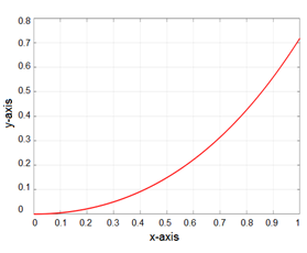
Now we get the results through the MATLAB solution to show the solutions method in the first example as in Figure 1.
Figure 1. Comparison of solutions with the x-axis and y-axes for the first problem
$\begin{gathered}x=0: 0.001: 1 ; \\ \operatorname{Plot}\left(x, y \operatorname{Sol}(x), 'r^{\prime}, ' \text {line} \text { width }^{\prime}, 2\right) ; \\ \text { Grid on } \\ \text { X label }\left(' x-\text { axis }^{\prime}\right) \\ \text { Y label }\left(' y-\text { axis }^{\prime}\right)\end{gathered}$
System response as a function of time in MATLAB for x and y coordinates obviously, when the curve starts from zero to the maximum, the error percentage is very small for the values between zero and other points in the curve passes, we can observe the difference of MATLAB solutions from arch passing through the points as shown also Multon closed to MATLAB with problem of first rank.
Example 2. Solve the differential equation by using three numerical methods if we have distance 0.5 for the steep and the equation from second ordered equation.
$y^{\prime}=y-x^2+1, h=0.5, y_0=0.5$
If solving is y=(x+1)2-0.50.5ex
To find y4 by these numerical methods (Runge-Kutta, Bash forth, Moulton methods)?
Solution from:
$\begin{gathered}y=(x+1)^2-0.5 e^x, h=0.5 \\ y_1=\left(x_1+1\right)^2-0.5 e^{x_1}=1.425639 \\ y_2=\left(x_2+1\right)^2-0.5 e^{x_2}=2.640859 \\ y_3=\left(x_3+1\right)^2-0.5 e^{x_3}=4.009155\end{gathered}$
(1) Solution of example 2 by using Runge-Kutta method
$y_{i+1}=y_i+\frac{1}{6}\left(k_1+2 k_2+2 k_3+k_4\right)$
Such that: $k_1=h f\left(x_i+y_i\right), k_2=h f\left(x_i+\frac{h}{2}, y_i+\frac{k_1}{2}\right)$, $k_3=h f\left(x_i+\frac{h}{2}, y_i+\frac{k_2}{2}\right), k_4=h f\left(x_i+h, y_i+k_3\right), y_4=$ $y_3+\frac{1}{6}\left(k_1+2 k_2+2 k_3+k_2\right)$, subtitling the values of $k$.
$\begin{aligned} & k_1=h\left(y_3-x_3^2+1\right)=1.379577 \\ & k_2=h\left(y_3+\frac{k_1}{2}-\left(x_3+\frac{h}{2}\right)^2+1\right)=1.318221 \\ & k_3=h\left(y_3+\frac{k_2}{2}-\left(x_3+\frac{h}{2}\right)^2+1\right)=1.302882 \\ & k_4=h\left(y_3+k_3-\left(x_3+h\right)^2+1\right)=1.156018 \\ & y_4=4.009155+\frac{1}{6}(1.37957+2(1.3118221) \\ &+2(1.302882)+1.156018) \\ & y_4 =5.305455\end{aligned}$
(2) Using Bash Forth method for solving example 2
$\begin{aligned} & y_4=y_3+\frac{h}{24}\left[55 f_3-59 f_2+37 f_1-9 f_0\right] \\ & f(x, y)=y-x^2-1 \\ & f_0=f\left(x_0, y_0\right)=f(0,0.5)=y_0-x_0^2+1=0.5-0+1 \\ & \quad=1.5 \\ & f\left(x_1, y_1\right)=y_1-x_1^2+1=2.175639 \\ & f\left(x_2, y_2\right)=y_2-x_2^2+1=2.640859 \\ & y_4=4.009155+\frac{0.5}{24}[55(2.759155)-59(2.640859) \\ & \quad+37(2.175639)-9(1.5)] \\ & y_4=5.32043598\end{aligned}$
(3) Using Moulton method to solve example 2
$\begin{aligned} & y_4=y_3+\frac{h}{24}\left[9 f_4+19 f_3-5 f_2+f_1\right] \\ & f(x, y)=y-x^2-1 \\ & f\left(x_1, y_1\right)=y_1-x_1^2+1=2.175639 \\ & f\left(x_2, y_2\right)=y_2-x_2^2+1=2.640859 \\ & f\left(x_3, y_3\right)=y_3-x_3^2+1=2.750155 \\ & f\left(x_4, y_4\right)=y_4-x_4^2+1=2.305455 \\ & y_4=4.009155+\frac{0.5}{24}[9(2.305455)+19(2.305455)-5(2.640859+2.175639)] \\ & y_4=5.303829 \quad\end{aligned}$
(4) Using MATLAB Ode45 methods to solve second example
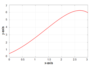
$ clc\\ Clear\\ Close all \\ syms \,\, y(x) \\ Ode=\operatorname{diff}(y, x)=y-x^2+1; \\ cond=y(0)=0.5; \\ y \,\, Sol (x)=dsolve (ode, cond); \\ ans=6.158753 \\ x=0: 0.001: 3; \\ Plot \left(x, y\right. Sol (x),{ }^{\prime} r^{\prime}, 'line width', 2 ); \\ Grid on \\ X\,\, label ('x-axis') \\Y \,\, label \left(' y-a x i s^{\prime}\right)$
Table 2. The results of three numerical methods with MATLAB its clear by Figure 2
|
yi |
Bash Forth |
Moulton |
Runge-Kutta |
MATLAB (ODE45) |
|
y4 |
5.320435 |
5.303829 |
5.305455 |
6.158753 |
Discussion results of the second example, as well as Moulton with MATLAB'S have the best approximation, and Runge-Kutta with Bash forth are close together, as shown earlier in Table 2 with a first order example.
Results of the second squared example with the quadratic function and the exponential function, we notice through numerical solutions that appeared to us that the results of Runge-Kutta method are close to Moulton. Also, the solutions of Adams-Bash forth method are close solutions of MATLAB. Therefore, we can say here that solutions of the Adams-Bash forth method are preferred with the quadratic function and the exponential function.
Figure 2. System response as a function of time using MATLAB solutions and numerical methods as shown in the diagram with both axis
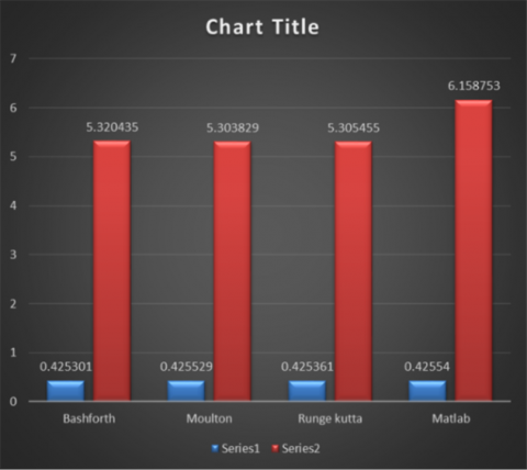
Figure 3. Comparison of the methods, Bash forth, Moulton, Kutta, and MATLAB
The results start from the value 0.5 during each point. In the first figure in blue columns, represent the results for solutions of the first example, and the second, represented by the red columns, are the results of the second example. We represented the solutions for two examples, from the first to last value, as in the fig on both axes (Figure 3). In first example with step h=0.2 at first order function, the blue column in the model represents a unit solution with first order differential equations and three numerical methods. Also, with four steps in solutions we get a good approximation of all steps. Small errors. For each method, also compared four values as shown in the blue column and red column as in the third figure. First, we compare the values of the blue column which it turns out, that Moulton's method is better than other numerical solutions used in the first problem. Also, for second example when h=0.5 with quadratic and exponential equations which gives excellent results in the red color of Moulton's column it has a better approximation than other methods, it has a small error of the MATLAB method, and also with two numerically different solutions for kinds of equations where Moulton gives the best approximation rest of numerical methods is closer to MATLAB solutions with the problem of first order but with the second order bash forth is the winner.
Our article is mainly about the Adams-Bashforth, Rung-Kutt-4, and Moulton as approximation numerical methods using MATLAB, which is solved in the first and second order also Moulton stay winner method on first example. But in the second part the methods modified by Adams-Bashforth-Moulton and MATLAB, we prove the main argument by applying inequalities and avoiding using higher order with other methods only by Adams-Bashforth achieved profitable results with the highest order, moreover Rung-Kutta-4, and MATLAB gives positive results with all the solutions. Finally, we recommend using Adams-Bashforth with the highest order and Moulton with first rank the MATLAB stay the best with all ranks have profitable results.
[1] Daroczy, G., Wolska, M., Meurers, W.D., Nuerk, H.C. (2015). Word problems: A review of linguistic and numerical factors contributing to their difficulty. Frontiers in Psychology, 6: 348. https://doi.org/10.3389/fpsyg.2015.00348
[2] Shukla, A., Vijayakumar, V., Nisar, K.S. (2022). A new exploration on the existence and approximate controllability for fractional semilinear impulsive control systems of order r∈(1, 2). Chaos, Solitons Fractals, 154: 111615. https://doi.org/10.1016/j.chaos.2021.111615
[3] Bansal, M., Goyal, A., Choudhary, A. (2022). A comparative analysis of K-nearest neighbor, genetic, support vector machine, decision tree, and long short term memory algorithms in machine learning. Decision Analytics Journal, 3: 100071. https://doi.org/10.1016/j.dajour.2022.100071
[4] AlShurbaji, M., Kader, L.A., Hannan, H., Mortula, M., Husseini, G.A. (2023). Comprehensive study of a diabetes mellitus mathematical model using numerical methods with stability and parametric analysis. International Journal of Environmental Research and Public Health, 20(2): 939. https://doi.org/10.3390/ijerph20020939
[5] Keller, R.T., Du, Q. (2021). Discovery of dynamics using linear multistep methods. SIAM Journal on Numerical Analysis, 59(1): 429-455. https://doi.org/10.1137/19M130981X
[6] Kazakov, E., Efremenko, D., Zemlyakov, V., Gao, J. (2022). A time-parallel ordinary differential equation solver with an adaptive step size: Performance assessment. In Russian Supercomputing Days, pp. 3-17. https://doi.org/10.1007/978-3-031-22941-1_1
[7] Maclean, J., Bunder, J.E., Roberts, A.J. (2021). A toolbox of equation-free functions in Matlab/Octave for efficient system level simulation. Numerical Algorithms, 87(4): 1729-1748. https://doi.org/10.1007/s11075-020-01027-z
[8] Raja, M.A.Z., Sabati, M., Parveen, N., Awais, M., Awan, S.E., Chaudhary, N.I., Alquhayz, H. (2021). Integrated intelligent computing application for effectiveness of Au nanoparticles coated over MWCNTs with velocity slip in curved channel peristaltic flow. Scientific Reports, 11(1): 22550. https://doi.org/10.1038/s41598-021-98490-y
[9] Awan, S.E., Raja, M.A.Z., Gul, F., Khan, Z.A., Mehmood, A., Shoaib, M. (2021). Numerical computing paradigm for investigation of micropolar nanofluid flow between parallel plates system with impact of electrical MHD and Hall current. Arabian Journal for Science and Engineering, 46: 645-662. https://doi.org/10.1007/s13369-020-04736-8
[10] Hasan, M.S., Mondal, R.N., Lorenzini, G. (2019). Centrifugal instability with convective heat transfer through a tightly coiled square duct. Mathematical Modelling of Engineering Problems, 6(3): 397-408. https://doi.org/10.18280/mmep.060311
[11] Deniz, F.N., Alagoz, B.B., Tan, N., Koseoglu, M. (2020). Revisiting four approximation methods for fractional order transfer function implementations: Stability preservation, time and frequency response matching analyses. Annual Reviews in Control, 49: 239-257. https://doi.org/10.1016/j.arcontrol.2020.03.003
[12] Kuttler, C., Maslovskaya, A. (2021). Hybrid stochastic fractional-based approach to modeling bacterial quorum sensing. Applied Mathematical Modelling, 93: 360-375. https://doi.org/10.1016/j.apm.2020.12.019
[13] Hopkins, M., Mikaitis, M., Lester, D.R., Furber, S. (2020). Stochastic rounding and reduced-precision fixed-point arithmetic for solving neural ordinary differential equations. Philosophical Transactions of the Royal Society A, 378(2166): 20190052. https://doi.org/10.1098/rsta.2019.0052
[14] Sun, X., Zheng, X., Li, D. (2013). Recent advances in mathematical programming with semi-continuous variables and cardinality constraint. Journal of the Operations Research Society of China, 1(10): 55-77. https://doi.org/10.1007/s40305-013-0004-0
[15] Abiodun, O.I., Jantan, A., Omolara, A.E., Dada, K.V., Mohamed, N.A., Arshad, H. (2018). State-of-the-art in artificial neural network applications: A survey. Heliyon, 4(11): e00938. https://doi.org/10.1016/j.heliyon.2018.e00938
[16] Peinado, J., Ibáñez, J., Arias, E., Hernández, V. (2010). Adams-Bashforth and Adams-Moulton methods for solving differential Riccati equations. Computers and Mathematics with Applications, 60(11): 3032-3045. https://doi.org/10.1016/j.camwa.2010.10.002
[17] Khane Keshi, F., Moghaddam, B.P., Aghili, A. (2019). A numerical technique for variable-order fractional functional nonlinear dynamic systems. International Journal of Dynamics and Control, 7(4): 1350-1357. https://doi.org/10.1016/j.aeue.2017.11.019
[18] Calvo, M.P., Palencia, C. (2006). A class of explicit multistep exponential integrators for semilinear problems. Numerische Mathematik, 102(3): 367-381. https://doi.org/10.1007/s00211-005-0627-0
[19] Luan, V.T., Ostermann, A. (2014). Exponential rosenbrock methods of order five-Construction, analysis and numerical comparisons. Journal of Computational and Applied Mathematics, 255: 417-431. https://doi.org/10.1016/j.cam.2013.04.041
[20] Qin, C., Tao, J., Li, L., Liu, C. (2017). An Adams-Moulton-based method for stability prediction of milling processes. The International Journal of Advanced Manufacturing Technology, 89(9): 3049-3058. https://doi.org/10.1007/s00170-016-9293-x
[21] Misirli, E., Gurefe, Y. (2011). Multiplicative adams bashforth-moulton methods. Numerical Algorithms 57: 425-439. https//doi.org/10.1007/s11075-010-9437-2
[22] Pan, Y., He, Y., Mikkola, A. (2019). Accurate real-time truck simulation via semirecursive formulation and Adams–Bashforth–Moulton algorithm. Acta Mechanica Sinica, 35: 641-652. https://doi.org/10.1007/s10409-018-0829-1
[23] Rosenfeld, J.A., Dixon, W.E. (2017). Approximating the caputo fractional derivative through the mittag-leffler reproducing kernel hilbert space and the kernelized adams--bashforth--Moulton method. SIAM Journal on Numerical Analysis, 55(3): 1201-1217. https://doi.org/10.1137/16M1056894
[24] Jeng, S.W., Kilicman, A. (2020). Series expansion and fourth-order global Padé approximation for a rough heston solution. Mathematics, 8(11): 1968. https://doi.org/10.3390/math8111968
[25] Hochbruck, M., Ostermann, A. (2011). Exponential multistep methods of Adams-type. BIT Numerical Mathematics, 51(4): 889-908. https://doi.org/10.1007/s10543-011-0332-6
[26] Hochbruck, M., Ostermann, A. (2010). Exponential integrators. Acta Numerica, 19: 209-286. https://doi.org/10.1017/S0962492910000048
[27] Ali, A.J., Abbas, A.F. (2022). Applications of numerical integrations on the trapezoidal and Simpson's methods to analytical and MATLAB solutions. Mathematical Modelling of Engineering Problems, 9(5): 1352-1358. https://doi.org/10.18280/mmep.090525
[28] Yushkova, M., Sanchez, A., de Castro, A. (2021). Strategies for choosing an appropriate numerical method for FPGA-based HIL. International Journal of Electrical Power & Energy Systems, 132: 107186. https://doi.org/10.1016/j.ijepes.2021.107186
[29] Shawagfeh, N., Kaya, D. (2004). Comparing numerical methods for the solutions of systems of ordinary differential equations. Applied Mathematics Letters. 17(3): 323-328. https://doi.org/10.1016/S0893- 9659(04)90070-5
[30] Din, A., Shah, K., Seadawy, A., Alrabaiah, H., Baleanu, D. (2020). On a new conceptual mathematical model dealing the current novel coronavirus-19 infectious disease. Results in Physics, 19: 103510. https://doi.org/10.1016/j.rinp.2020.103510