Naga Jagadesh Bommagani*![]() | Asha Venkataramana
| Asha Venkataramana![]() | Rashmi Vemulapalli
| Rashmi Vemulapalli![]() | Tejesh Reddy Singasani
| Tejesh Reddy Singasani![]() | Alok Kumar Pani
| Alok Kumar Pani![]() | Manjunatha Basavannappa Challageri
| Manjunatha Basavannappa Challageri![]() | Saikumar Kayam
| Saikumar Kayam![]()
© 2024 The authors. This article is published by IIETA and is licensed under the CC BY 4.0 license (http://creativecommons.org/licenses/by/4.0/).
OPEN ACCESS
Human activity recognition (HAR) is a focal point of study in the realms of human perception and computer vision due to its widespread applicability in various contexts, such as intelligent video surveillance, ambient assisted living, HCI, HRI, IR, entertainment, and intelligent driving. With the prevalence of deep learning techniques for image classification, researchers have shifted away from the labor-intensive practice of hand-crafting in favor of these methods in HAR. However, Convolutional Neural Networks (CNNs) face challenges such as the receptive field problem and limited sample issues that remain unsolved. This paper introduces a two-branch convolutional neural network for HAR classification, incorporating a polarized full attention method to address the aforementioned issues. The Artificial Butterfly Optimization (ABO) is employed for optimal hyper-parameter tuning. The proposed network utilizes two-branch CNNs to efficiently extract data, simplifying convolutional layers' kernel sizes to enhance network training and suitability for low-data settings. Feature extraction effectiveness is improved by implementing the one-shot assembly method. To amalgamate feature maps and provide global context, an enhanced full attention block called polarized full attention is utilized. Experimental results demonstrate the superiority of the proposed model in detecting human behaviors on the LoDVP Abnormal Behaviors dataset and the UCF50 dataset. Furthermore, the suggested model is adaptable to incorporate new sensor data, making it particularly valuable for real-time human activity identification applications. The Recall is 100 for the 1st dataset, 94 for the 2nd dataset, and 100 for the 3rd dataset, respectively. The F1-Score is 96.61836 for the 1st dataset, 96.90722 for the 2nd dataset, and 98.03922 for the 3rd dataset, respectively.
convolutional neural networks, artificial butterfly optimization, human activity recognition, polarized full attention mechanism, one-shot learning
Human activity recognition (HAR) in the home, achieved by establishing a network of sensors to detect human behavior, can enhance people's ability to maintain independence and quality of life [1]. HAR is a dynamic and complex research area [2-4], driven by the increasing demand for medical diagnosis of chronic diseases, active home automation [5], and convenient services. Methods based on affordable and user-friendly sensors for monitoring and recording human daily actions can eliminate the constraints of human subjectivity. Doctors can gain insights into managing patients with chronic illnesses by reviewing data collected from patients' daily activity logs. Thanks to sensor devices, patients can undergo continuous monitoring and treatment even in the absence of medical professionals. However, other internal variables significantly impact human health and quality of life.
HAR serves as the primary method for integrating smart sensor monitoring equipment into the natural surroundings of a smart environment. Research challenges with practical implications [6] arise from the complexity of sensor data across various configurations and locations. Issues include determining how to use the features of sensor data to extract discriminating characteristics and how to enhance reliability based on sensor data.
Human behavior is unpredictable, influenced by individual differences in taste and lifestyle habits. When a sensor used for feature acquisition cannot discern a subject's primary characteristics, extracting the subject's behavior feature space becomes challenging. Implementing human body tracking technology in a visual sensor ensures constant visibility of the subject. However, visual monitoring involves large data volumes, making it resource-intensive to process, with privacy leaks being a concern [7]. Wearable sensors, while providing reliable data collection, have drawbacks such as being cumbersome and difficult to use for extended periods, limiting their suitability for identifying complex activities [8].
Integrated multitype sensors placed in the subject's environment track the current status of the smart space and gather data about the inhabitants without disruption [9]. However, environmental sensors may introduce noise data into the stream, impacting feature definition [10]. Analyzing features from different datasets and identifying significant aspects of behaviors can aid in optimizing the selection and deployment of environmental sensors [11], leading to improved recognition accuracy and more precise conclusions when combined with high-quality data feature sets.
Significant intraclass and modest interclass variances affect the classifier's performance in activity detection. Time-stamped streams of sensor activations are often presented as gathered data [12], segmented into activity instances represented by sequences of sensor events [13]. Two types of techniques for extracting HAR features from sensor sequence instances are conventional feature extraction and expression techniques [14]. Conventional methods require manual extraction of time domain features and other feature vectors [15], providing only superficial characteristics. Deep learning technology, without human interaction, can automatically extract richer and more nuanced characteristics from raw data, efficiently resolving intraclass differences and interclass similarities [16].
In the proposed scheme, spectral and spatial information of HAR are separately extracted using a two-branch structure. To adapt the network to small sample contexts, complexity is reduced by minimizing the window widths of the 3D layers. Additionally, the network's convolutional layers are connected using a one-time connection, allowing the shallow layers to be retained in the upper layers and retrieved with deep semantic features. This one-time connection benefits the network's ability to extract feature maps across layers and effectively extract training-sample features. The use of Batch Normalization (BN) layers and Parametric Rectified Linear Unit (PReLU) layers mitigates the gradient problem and network degradation. After the two-branch, an enhanced full attention (FLA) mechanism is adopted to combine spectral and spatial characteristics acquired from the two-branch network. The Artificial Butterfly Optimization Algorithm (ABOA) handles the fine-tuning process.
The rest of the paper is organized into five sections: 2. Background Work; 3. Proposed Method; 4. Investigation and Discussion of Results; and 5. Conclusion.
Adaptively limiting sensor noise in smart home situations is made possible by the strategy developed by Li et al. [17]. For HAR, they suggest using a sensor status frequency-inverse type frequency to conduct a contribution significance analysis (CSA). This strategy is used to evaluate the effectiveness of a certain sensor in recognizing a specific activity. Next, we use the arrangement of ambient sensors to create a spatial distance matrix for improved awareness of context and quieter data. Finally, we present a HAR method for everyday behavior detection that makes use of a broad time-domain network and input from several sensor environments. Experiments conducted on the CASAS dataset reveal that the projected HAR_WCNN attains better results than the state-of-the-art approaches compared to it when it comes to HAR accuracy and runtime.
A novel deep learning-based approach, dubbed HAR-DeepConvLG, is suggested by Ding et al. [18]. To accurately learn blocks, the extracted features are fed into three parallel routes, each consisting of a long short-term memory (LSTM) layer, to learn temporal representations. To solve the vanishing gradient issue, the three routes are connected in parallel. Finally, tests were run on four popular HAR datasets to assess the performance of the proposed approach. The efficiency of the model was further demonstrated by comparing it to numerous state-of-the-art models. Compared to other HAR deep learning-based models, the proposed HAR-DeepConvLG model achieves competitive classification accuracy, as shown by experimental findings.
In order to construct a reliable HAR system using data collected by wearable sensors, Helmi et al. [19] have integrated the requirements of both DL and SI. Residuals are used to create a lightweight feature extraction approach. New feature selection methods using the MPA are created to help choose the best features for inclusion in models. For this purpose, in addition to the original MPA, three binary differences are created: the MPA, the MPA, and the MPA. To guarantee the quality of performance of the MPA versions, we compare them against a number of other optimization algorithms using a wide range of evaluation indicators and conduct statistical analyses. We find that MPA performed the best out of all the MPA variations and other methodologies we looked at.
Using a multi-fusion procedure for multimodal human activity recognition, Dua et al. [20] propose a CNN and Gated Recurrent Unit (GRU) hybrid, "ICGNet," for HAR. The proposed network employs a CNN block inspired by the well-known Inception component. By applying convolutional filters of varying sizes simultaneously, the model can pick up details in the data at different levels of detail. To assist the model in retrieving useful information concealed across channels, it uses 1×1 convolution to pool the input across the channel dimension. The proposed ICGNet, by combining CNN and GRU, is better able to detect both short- and long-term series. It's an end-to-end approach for HAR that processes raw data from wearable sensors automatically, without the need for human intervention in feature engineering. HCI disciplines such as interactive gaming, robot learning, health monitoring, and pattern-based surveillance can all benefit from the proposed HAR system's integration of adaptive user interfaces. The average accuracy for MHEALTH and PAMAP2 datasets is 99.25% and 97.64%, respectively.
In order to make good use of temporal series data, Mim et al. [21] have presented a model they call the Gated Recurrent Unit-Inception (GRU-INC) model. The suggested model had an F1-score of 96.27% on the UCI-HAR dataset, 90.05% on the OPPORTUNITY dataset, 90.30% on the PAMAP2 dataset, 99.12% on the WISDM dataset, and 95.99% on the Daphnet dataset. The temporal component of the model makes use of the Generative Recurrent Unit (GRU) and the Attention Mechanism (AM), while the spatial component makes use of the Inception module and Block Attention Module (CBAM). We compared the suggested design to the current gold standard and other research in the field. The GRU-INC model has a greater recognition rate and reduced computational cost, as has been demonstrated. Therefore, our methodology may find use in activity-related clinical and therapeutic settings.
To effectively process feature vectors in a hierarchical fashion, Park et al. [22] present a deep learning-based HAR model they call MultiCNN-FilterLSTM, which integrates multihead through a residual link. To this purpose, we suggest a unique way of employing LSTM cells—referred to as filterwise LSTM, or FilterLSTM—so that the HAR model may discover the interdependencies between characteristics across multiple tiers of the hierarchy. Two publicly available datasets have been used to test the projected HAR model extensively. In contrast to state-of-the-art models, the suggested HAR prototype improves classification accuracy by 2.3%-4.4% while using 21%-70% fewer operations. For additional deployment study, the suggested model is also installed on a Raspberry Pi 4. Experiments are shown to prove that the suggested HAR model outdoes the state-of-the-art models when it comes to taking advantage of hierarchical linkages, and they provide crucial insights into how well the projected FilterLSTM works from the point of view of the IoT scheme.
3.1 Description of the datasets
Here, we'll go through the datasets that were employed. LoDVP Abnormal Activities, UCF50, and MOD20 datasets were used to achieve comprehensive experimental findings.
3.1.1 UCF50 dataset
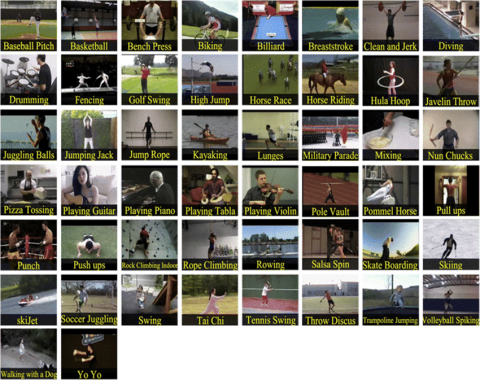
The 50 different types of actions that made up the UCF50 dataset. The dataset included authentic YouTube videos included. Camera movement, clutter, lighting, etc. all varied greatly across the sample. The videos grouped together may all center around the same character or have a similar setting or point of view. Figure 1 displays the UCF50 dataset.
Figure 1. Instance of the UCF50 dataset [23]
There were 50 different categories of data in the UCF50 dataset. The dataset includes events like a baseball pitch, a basketball shot, a billiards break, a clean and jerk, a dive, a drum solo, a fencing stroke, a golf swing, a guitar solo, a horse race, a horseback ride, a high jump, a horseback ride, a hula hoop, a rope, a jumping jack, a kayak Indoor rock climbing, rowing, salsa spins, skateboarding, skiing, skijet, juggling soccer balls, swing dancing, playing the tabla, tai chi, swing tennis, playing the violin, spiking volleyball, walking a dog, and yo-yoing are all in the list of 24 activities.
Both datasets were used to train the network, and the consequences were associated. The dataset was split into 10 layers. The smaller dataset is known as UCF50mini. The whole and reduced datasets were split into three groups: the training set.
3.1.2 LoDVP abnormal activities dataset
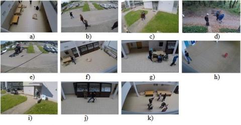
There are 1069 clips in all that make up the LoDVP Abnormal Activity collection. Videos depicting fictitious situations staged by amateur actors. The database contains only credible videos. The parking lot, woods have all been cited as sites of incidents. Multiple camera views of the scenes were taken. There are around 100 movies in each of the 11 categories that make up the dataset. The incident determines how long the video is, which might range from 1 second to 30 seconds. Characteristics shared among videos of the same type include a similar scenario, camera angle, and recurrent characters [24].
Figure 2. LoDVP Abnormal Events dataset: (a) Begging; (b) Drunkenness; (c) Fight; (d) Harassment; (e) Hijacking; (f) Knife danger; (g) Regular movies; (h) Pollution, (i) Pollution broken things; (j) A theft; (k) Terrorist acts [25]
Figure 2 displays the many categories that make up the LoDVP Abnormal Activity dataset. This dataset, like UCF50mini, was split into a training test and an authentication set for our work. The breakdown was as follows: 70%; 0%; 10%.
3.1.3 MOD20 dataset
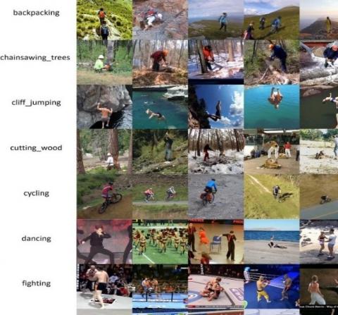
Six films were shot with a quadrotor UAV, while the remaining 2318 were pulled from YouTube to make up the MOD20 dataset. Media files are all full screen. The frame rate of the videos was below 29.97 fps. Both stationary and mobile cameras were used to capture the videos included in the dataset. Twenty different subject areas are included in the movies (see Figure 3) [26].
3.2 Classification
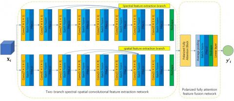
In this work, a two-branch network is proposed to extract the rich spectral and spatial information present in HAR. Figure 4a depicts the process flow of the projected network. The two-branch network make up the suggested network.
The spectrum information is extracted along the spectral dimension, while the spatial information is extracted along the spatial dimension, in a two-branch spectral-spatial network.
There are eight convolutional layers in the spectral feature extraction sub-branch, including the BN layer and the PReLU activation layer. We begin by increasing the number of feature maps and decreasing the spectral dimension using a layer with a window size of 711. After that, a total of five convolutional layers are employed to further extract the spectral information, each with a 711-window size. These convolutional layers save their prior feature maps thanks to a one-time link between them. The feature maps are then compressed using a size of 111. Additionally, the spectral dimension is layer with a C11 window size and a reshape operation. Similarly, eight convolutional layers are used in the spatial feature extraction sub-branch, utilizing BN and PReLU. To accomplish both of these goals, a convolutional layer with a 711-window size is first developed. After that, we reduce the spectral dimension by using a convolutional layer with a window size of C11. The spatial info is then extracted using layers with a 133-window size. These convolutional layers are connected by a one-time link to preserve the data. After that, the dimensionality of the spectrum is reduced and the number of feature mappings is compressed using a layer with a window size of 111. The final feature maps are a combination of the spectral branch's and the spatial branch's outputs.
Figure 3. The instance of the MOD20 dataset [26]
(a) The way the PTCN works
(b) The way the PFLA works
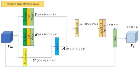
Figure 4. How the suggested network is put together
After extraction network has been deployed, the fusion network is utilized to fuse the resulting feature maps to provide accurate classifications. According to Figure 4(a), the layer makes up the polarized full network. To begin, the PFLA is used to supplement the feature maps generated by the self-attention mechanism of the preceding two-branch network. When fusing the channel-wise attentions, the proposed PFLA differs from the conventional FLA in that it uses a convolutional layer with an 11-window size to provide Sigmoid process to offer polarizability while maintaining high internal resolution. Figure 4(b) depicts the PFLA's process flow. The PFLA is similar to the FLA in most respects, with the exception that the Sigmoid process is used after the matrices V and A have been multiplied. After that, the spatial dimension is compressed and the features are fused using a regular pooling layer equipped with a BN layer and a PReLU layer. The spatial dimension is then compressed using a reshape operation, and the final classification results are produced via a Linear layer. The dataflows network with Xi=R=110399 as input data are provided in Tables 1-3 to provide an overview of the proposed network. The suggested network is trained using an expression for cross entropy loss.
$L_i=-\left[y_i \log _i^{\prime}+\left(1-y_i\right) \log \left(1-y_i^{\prime}\right)\right]$ (1)
Table 1. The dataflow of extraction outlet
|
Input Size |
Filters |
Layer Name |
Kernel |
Padding |
Output Size |
|
(24, 49, 9, 9) |
24 |
Conv |
(49, 1, 1) |
(0, 0, 0) |
(24, 1, 9, 9) |
|
(24, 1, 9, 9) |
- |
Reshape |
- |
- |
(24, 9, 9) |
|
(1, 103, 9, 9) |
24 |
Conv |
(7, 1, 1) |
(0, 0, 0) |
(24, 49, 9, 9) |
|
(24, 49, 9, 9) |
24 |
Conv |
(7, 1, 1) |
(3, 0, 0) |
(24, 49, 9, 9) |
|
(24, 49, 9, 9) |
24 |
Conv |
(7, 1, 1) |
(3, 0, 0) |
(24, 49, 9, 9) |
|
(24, 49, 9, 9) |
24 |
Conv |
(7, 1, 1) |
(3, 0, 0) |
(24, 49, 9, 9) |
|
(24, 49, 9, 9) |
24 |
Conv |
(7, 1, 1) |
(3, 0, 0) |
(24, 49, 9, 9) |
|
(24, 49, 9, 9) |
24 |
Conv |
(7, 1, 1) |
(3, 0, 0) |
(120, 49, 9, 9) |
|
(120, 49, 9, 9) |
24 |
Conv |
(1, 1, 1) |
(0, 0, 0) |
(24, 49, 9, 9) |
Table 2. The dataflow of the extraction division
|
Input Size |
Kernel |
Stride |
Padding |
Layer |
Filters |
Output Size |
|
(1, 103, 9, 9) |
(7, 1, 1) |
(3, 1, 1) |
(0, 0, 0) |
Name |
24 |
(24, 49, 9, 9) |
|
(24, 49, 9, 9) |
(49, 1, 1) |
(1, 1, 1) |
(0, 0, 0) |
Conv |
24 |
(24, 1, 9, 9) |
|
(24, 1, 9, 9) |
(1, 3, 3) |
(1, 1, 1) |
(0, 1, 1) |
Conv |
24 |
(120, 1, 9, 9) |
|
(120, 1, 9, 9) |
(1, 1, 1) |
(1, 1, 1) |
(0, 0, 0) |
Conv |
24 |
(24, 1, 9, 9) |
|
(24, 1, 9, 9) |
- |
- |
- |
Conv |
- |
(24, 9, 9) |
|
(24, 1, 9, 9) |
(1, 3, 3) |
(1, 1, 1) |
(0, 1, 1) |
Conv |
24 |
(24, 1, 9, 9) |
|
(24, 1, 9, 9) |
(1, 3, 3) |
(1, 1, 1) |
(0, 1, 1) |
Conv |
24 |
(24, 1, 9, 9) |
|
(24, 1, 9, 9) |
(1, 3, 3) |
(1, 1, 1) |
(0, 1, 1) |
Conv |
24 |
(24, 1, 9, 9) |
|
(24, 1, 9, 9) |
(1, 3, 3) |
(1, 1, 1) |
(0, 1, 1) |
Conv |
24 |
(24, 1, 9, 9) |
Table 3. The dataflow of the separated full attention features fusion system
|
Input Size |
Layer Name |
Kernel |
Filters |
Stride |
Padding |
Output Size |
|
(48, 1, 1) |
Reshape |
- |
- |
- |
- |
(48) |
|
(48) |
Linear |
- |
9 |
- |
- |
(9) |
|
(48, 9, 9) |
PFLA |
- |
- |
- |
- |
(48, 9, 9) |
|
(48, 9, 9) |
Avgpool |
- |
- |
- |
- |
(48, 1, 1) |
3.2.1 Hyper-parameter tuning using artificial butterfly algorithm
The territoriality of butterflies provides a useful model system in which to examine the effects of life history optimization on the lifetime cost of aggressive behavior [27]. A novel optimization technique can woodlands. We introduced the Artificial Butterfly Optimization (ABO) technique, which is inspired by the mating behavior of woodlands. Table 4 presents the ABO algorithm's pseudo code. The ABO procedure follows several criteria that idealize the butterflies' methods of mating:
a) In order to increase their chances of seeing butterflies strive to move into a better position known as a sunspot.
b) Every butterfly on a sunspot is constantly looking to move to a more favourable location on the sun.
c) Every canopy butterfly, in a never-ending competition for the sunspot, flies straight at any sunspot butterfly.
Table 4. Pseudo code of ABO algorithm
|
1. Initialize the locations of butterfly population 2. Evaluate the fitness of every butterfly 3. While not meet the terminal condition 4. Sort all butterflies by their fitness 5. Select some butterflies with better fitness to form sunspot butterflies, the rest form canopy butterflies 6. For each sunspot butterfly fly to one new location according to sunspot flight mode Evaluate the fitness of the new sunspot apply greedy selection on the original location and the new one End for 7. For each canopy butterfly Fly to one randomly selected sunspot butterfly according to canopy flight mode Evaluate the fitness 8. If better fitness Apply greedy selection on the original location and the new one 9. else Fly to new location according to free flight mode End if |
In Table 4, you'll see how the original population of butterflies was divided into a healthier and a less healthy subset. A separate flight plan is prepared for each party. There are now some similarities to niching approaches. It is standard practice to modify the behavior of a classical procedure using a niching technique [28, 29] to maintain distinct groups within the chosen populace component in order to effectively identify several optimum solutions. You may choose among the sunspot, canopy, or free flight modes. For these configurations, a wide range of flight methods is at your disposal. In other words, ABO may yield a new algorithm whenever one of the three flight manners is given a unique flying strategy.
Here are three distinct butterfly flying scenarios. In this research, we use a D- vector to characterize the site of a digital butterfly.
According to Eq. (2), each butterfly at random. This tactic is implemented in the ABO mode.
$X_{i_i}^{t+1}=X_{i, j}^t+\left(X_{i, j}^t-X_{k, j}^t\right) \cdot$ rand () (2)
In this play, I butterfly. In this expression, j is a dimension index selected at accidental among [1,D], t is the iteration count, rand() generates an among [-1,1], and k is a butterfly generated at random. Here, k is different from i.
Each direction picked at random by a neighbor according to Eq. (3). This strategy is utilized by both the flight modes of the ABO procedure.
$X_i^{t+1}=X_i^t+\frac{X_k^t-X_i^t}{\left\|X_k^t-X_i^t\right\|} \cdot(U b-L b)$. step $\cdot$ rand () (3)
where, i is the replicated, t is the number of repetitions, $X_i^{t+1}$ is the butterfly's new position, step is an accidental value among 0 and 1, and k is a haphazardly selected butterfly. In this case, k is dissimilar to i. The butterfly has a flight range among Lb and Ub, where Lb value. The values of Lb and Ub are significant in this context.
According to Eq. (4), each butterfly randomly chosen neighbor. In the exploration phase, the same method has been used to look for a new-fangled place. This process is realized in the ABO flight mode.
$X_i^{t+1}=X_k^t-2 \cdot a \cdot \operatorname{rand}()-a \cdot D$ (4)
where, $X_i^{t+1}$ is the novel site of the ith digital produces an accidental value among 0 and 1, and a decrease linearly from 2 to 0 with each repetition. k is a butterfly generated using Eq. (5).
$D=\left|2 \cdot \operatorname{rand}() \cdot X_k^t-X_i^t\right|$ (5)
If i produces a random number among zero and one. The value of the step parameter in Eq. (2) is variable. As shown in Eq. (6), we employ a diminishing method. In a linear fashion, with cumulative iterations, step declines from 1 to stepe. A better step value in the beginning increases the global searching ability and variety. In the final phase, better convergence is achieved with smaller step values since massive leaping is avoided.
step $=1-\left(1-\right.$ step $\left._e\right) \cdot \frac{E}{\max E}$ (6)
where, E is present assessments total and maxE is the max assessments count.
Hardware-wise, the Intel Core I7-8300 K processor, 16 GB of RAM, and an Nvidia GeForce GTX1060 6 G provide a single computing platform. Python=3.6, are the supported versions of Python and other applications on Windows 10.
We employ the True Positive Rate (TPR), the True Negative Rate (TNR), the False Positive Rate (FPR), the False Negative Rate (FNR), and the Accuracy of action detection rate to measure the efficacy of our suggested method.
$T P R=T P /(T P+F N)$ (7)
$T N R=T N /(T N+F P)$ (8)
$F P R=F P /(F P+T N)$ (9)
$F N R=F N /(T P+F N)$ (10)
$Accuracy =T P+T N / N$ (11)
where, TP – True Positive; TN – True Negative; FP – False Positive; FN – False Negative; N – Number of Frames.
4.1 Presentation investigation of proposed model
In Table 5, we characterize the PTCN results. In this analysis, we include three different datasets, with the sum of testing frames in the 1st dataset as 150, the 2nd dataset as 150, and also the 3rd dataset as 150, respectively. The sum of True Positives (TP) in the 1st dataset is 90, in the 2nd dataset is 95, and in the 3rd dataset is 100, respectively. The sum of False Negatives (FN) in the 1st dataset is 10, in the 2nd dataset is 5, and in the 3rd dataset is 0, respectively. The True Positive Rate (TPR) in the 1st dataset is 90, in the 2nd dataset is 95, and in the 3rd dataset is 100, respectively. The False Negative Rate (FNR) in the 1st dataset is 10, in the 2nd dataset is 5, and in the 3rd dataset is 0, respectively. The sum of True Negatives (TN) in the 1st dataset is 43, in the 2nd dataset is 36, and in the 3rd dataset is 34, respectively. The sum of False Positives (FP) in the 1st dataset is 7, in the 2nd dataset is 14, and in the 3rd dataset is 16, respectively. The True Negative Rate (TNR) value in the 1st dataset is 86, in the 2nd dataset is 72, and in the 3rd dataset is 68, respectively. The False Positive Rate (FPR) in the 1st dataset is 14, in the 2nd dataset is 28, and in the 3rd dataset is 32, respectively. The Accuracy is 88.66667, 87.33333, and 89.33333 for the 1st, 2nd, and 3rd datasets, respectively. The Precision in the 1st dataset is 92.78351, in the 2nd dataset is 87.15596, and in the 3rd dataset is 86.2069, respectively. The Recall Rate in the 1st dataset is 90, and in the 3rd dataset is 95 and 100, respectively. The F1-score in the 1st dataset is 91.37056, in the 2nd dataset is 90.90909, and in the 3rd dataset is 92.59259, respectively.
Table 5. PTCN results
|
|
Dataset 1 |
Dataset 2 |
Dataset 3 |
|
No. of testing frames |
150 |
150 |
150 |
|
No. of TP's |
90 |
95 |
100 |
|
No. of FN's |
10 |
5 |
0 |
|
Sensitivity/TPR |
90 |
95 |
100 |
|
FNR |
10 |
5 |
0 |
|
No. of TN's |
43 |
36 |
34 |
|
No. of FP's |
7 |
14 |
16 |
|
Specificity/TNR |
86 |
72 |
68 |
|
FPR |
14 |
28 |
32 |
|
Accuracy |
88.66667 |
87.33333 |
89.33333 |
|
Precision |
92.78351 |
87.15596 |
86.2069 |
|
Recall |
90 |
95 |
100 |
|
F1-Score |
91.37056 |
90.90909 |
92.59259 |
Table 6. PFLA results
|
Dataset 1 |
Dataset 2 |
Dataset 3 |
|
|
No. of testing frames |
150 |
150 |
150 |
|
No. of TP's |
90 |
100 |
100 |
|
No. of FN's |
10 |
0 |
0 |
|
Sensitivity/TPR |
90 |
100 |
100 |
|
FNR |
10 |
0 |
0 |
|
No. of TN's |
50 |
39 |
41 |
|
No. of FP's |
0 |
11 |
9 |
|
Specificity/TNR |
100 |
78 |
82 |
|
FPR |
0 |
22 |
18 |
|
Accuracy |
93.33333 |
92.66667 |
94 |
|
Precision |
100 |
90.09009 |
91.7431193 |
|
Recall |
90 |
100 |
100 |
|
F1-Score |
94.73684 |
94.78673 |
95.6937799 |
In Table 6, we characterize the PFLA results. In the analysis, the amount of testing frames value is 150 for the 1st dataset, 150 for the 2nd dataset, and 150 for the 3rd dataset, respectively. The amount of True Positives (TP) is 90 for the 1st dataset, 100 for the 2nd dataset, and 100 for the 3rd dataset, respectively. The amount of False Negatives (FN) is 10 for the 1st dataset, 0 for the 2nd dataset, and 0 for the 3rd dataset, respectively. The Sensitivity/True Positive Rate (TPR) is 90 for the 1st dataset, 100 for the 2nd dataset, and 100 for the 3rd dataset, respectively. The False Negative Rate (FNR) is 10 for the 1st dataset, 0 for the 2nd dataset, and 0 for the 3rd dataset, respectively.
The number of True Negatives (TN) is 50 for the 1st dataset, 39 for the 2nd dataset, and 41 for the 3rd dataset, respectively. The number of False Positives (FP) is 0 for the 1st dataset, 11 for the 2nd dataset, and 9 for the 3rd dataset, respectively. The Specificity/True Negative Rate (TNR) is 100 for the 1st dataset, 78 for the 2nd dataset, and 82 for the 3rd dataset, respectively. The False Positive Rate (FPR) is 0 for the 1st dataset, 22 for the 2nd dataset, and 18 for the 3rd dataset, respectively.
The Accuracy is 93.33333 for the 1st dataset, 92.66667 for the 2nd dataset, and 94 for the 3rd dataset, respectively. The Precision is 100 for the 1st dataset, 90.09009 for the 2nd dataset, and 91.7431193 for the 3rd dataset, respectively. The Recall is 90 for the 1st dataset, 100 for the 2nd dataset, and 100 for the 3rd dataset, respectively. The F1-Score is 94.73684 for the 1st dataset, 94.78673 for the 2nd dataset, and 95.6937799 for the 3rd dataset, respectively.
In Table 7, the proposed hybrid model with ABO is analyzed. The sum of testing frames value is 150 for the 1st dataset, 150 for the 2nd dataset, and 150 for the 3rd dataset, respectively. The sum of True Positives (TP) is 100 for the 1st dataset, 94 for the 2nd dataset, and 100 for the 3rd dataset, respectively. The sum of False Negatives (FN) is 0 for the 1st dataset, 6 for the 2nd dataset, and 0 for the 3rd dataset, respectively. The Sensitivity/True Positive Rate (TPR) is 100 for the 1st dataset, 94 for the 2nd dataset, and 100 for the 3rd dataset, respectively. The False Negative Rate (FNR) is 0 for the 1st dataset, 6 for the 2nd dataset, and 0 for the 3rd dataset, respectively.
Table 7. Proposed hybrid model with ABO
|
Dataset 1 |
Dataset 2 |
Dataset 3 |
|
|
No. of testing frames |
150 |
150 |
150 |
|
No of TP's |
100 |
94 |
100 |
|
No of FN's |
0 |
6 |
0 |
|
Sensitivity/TPR |
100 |
94 |
100 |
|
FNR |
0 |
6 |
0 |
|
No. of TN's |
43 |
50 |
46 |
|
No. of FP's |
7 |
0 |
4 |
|
Specificity/TNR |
86 |
100 |
92 |
|
FPR |
14 |
0 |
8 |
|
Accuracy |
95.33333 |
96 |
97.33333 |
|
Precision |
93.45794 |
100 |
96.15385 |
|
Recall |
100 |
94 |
100 |
|
F1-Score |
96.61836 |
96.90722 |
98.03922 |
The sum of True Negatives (TN) is 43 for the 1st dataset, 50 for the 2nd dataset, and 46 for the 3rd dataset, respectively. The sum of False Positives (FP) is 7 for the 1st dataset, 0 for the 2nd dataset, and 4 for the 3rd dataset, respectively. The Specificity/True Negative Rate (TNR) is 86 for the 1st dataset, 100 for the 2nd dataset, and 92 for the 3rd dataset, respectively. The False Positive Rate (FPR) is 14 for the 1st dataset and 8 for the 2nd dataset, respectively.
The Accuracy is 95.33333 for the 1st dataset, 96 for the 2nd dataset, and 97.33333 for the 3rd dataset, respectively. The Precision is 93.45794 for the 1st dataset, 100 for the 2nd dataset, and 96.15385 for the 3rd dataset, respectively. The Recall is 100 for the 1st dataset, 94 for the 2nd dataset, and 100 for the 3rd dataset, respectively. The F1-Score is 96.61836 for the 1st dataset, 96.90722 for the 2nd dataset, and 98.03922 for the 3rd dataset, respectively.
4.2 Experimental analysis of different models
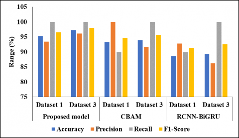
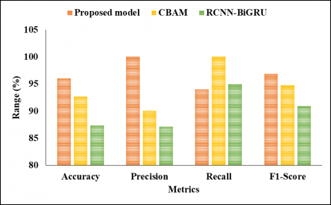
In Table 8, the comparison analysis of various representations with the recommended model is characterized. The proposed model's accuracy values were 95.33 for the 1st dataset as shown in Figure 5, 96 for the 2nd dataset as shown in Figure 6, and 97.33 for the 3rd dataset. The CBAM [20] model achieved an accuracy of 92.66 for the 1st dataset, 88.66 for the 2nd dataset, and 87.33 for the 3rd dataset, respectively. The RCNN-BiGRU [19] model obtained an accuracy of 94 for the 1st dataset, 94.78 for the 2nd dataset, and 95.69 for the 3rd dataset.
In terms of precision, the proposed model achieved values of 93.45 for the 1st dataset, 100 for the 2nd dataset, and 96.15 for the 3rd dataset. The CBAM [20] model had precision values of 90.09 for the 1st dataset, 91.74 for the 2nd dataset, and 92.78 for the 3rd dataset. The RCNN-BiGRU [19] model obtained precision values of 87.15 for the 1st dataset, 90.90 for the 2nd dataset, and 91.74 for the 3rd dataset.
For the Recall metric, the proposed model achieved values of 100 for the 1st dataset, 94 for the 2nd dataset, and 100 for the 3rd dataset. The CBAM [20] model had Recall values of 90 for the 1st dataset, 100 for the 2nd dataset, and 94.78 for the 3rd dataset. The RCNN-BiGRU [19] model obtained Recall values of 90 for the 1st dataset, 94.73 for the 2nd dataset, and 100 for the 3rd dataset.
Furthermore, the F1-Score for the proposed model was 96.61 for the 1st dataset and 96.90 for the 2nd dataset. The CBAM [20] model achieved F1-Score values of 91.37 for the 1st dataset, 90.90 for the 2nd dataset, and 92.59 for the 3rd dataset. The RCNN-BiGRU [19] model obtained F1-Score values of 94.73 for the 1st dataset, 94.78 for the 2nd dataset, and 95.69 for the 3rd dataset.
Table 8. Comparison analysis of various models with proposed model
|
Techniques |
Proposed Model |
CBAM [20] |
RCNN-BiGRU [19] |
||||||
|
Dataset |
Dataset 1 |
Dataset 2 |
Dataset 3 |
Dataset 1 |
Dataset 2 |
Dataset 3 |
Dataset 1 |
Dataset 2 |
Dataset 3 |
|
Accuracy |
95.33 |
96 |
97.33 |
93.33 |
92.66 |
94 |
88.66 |
87.33 |
89.33 |
|
Precision |
93.45 |
100 |
96.15 |
100 |
90.09 |
91.74 |
92.78 |
87.15 |
86.20 |
|
Recall |
100 |
94 |
100 |
90 |
100 |
100 |
90 |
95 |
100 |
|
F1-Score |
96.61 |
96.90 |
98.03 |
94.73 |
94.78 |
95.69 |
91.37 |
90.90 |
92.59 |
Figure 5. Graphical description of projected model with existing procedures
Figure 6. Analysis of numerous models on second dataset
In this study, we proposed a polarized full-attention process for use in a two-branch convolutional network for HAR organization. The suggested PTCN divides the feature extraction block into two distinct limbs, one for spectral extraction and another for spatial extraction. Convolutional layer kernel sizes are reduced for spectral and spatial feature extraction to minimize network complexity and accommodate the limited sample situation. Additionally, the suggested PTCN makes use of a one-shot connection to boost feature extraction performance under constrained training sample conditions. Furthermore, the attention process is utilized to identify salient abstract qualities capable of discrimination. To address the issue of feature fusion, we employ a new and enhanced full attention method called polarized full attention. When fusing spectral and spatial data, the attention mechanism can help the network retain its high internal resolution by providing polarizability. The effectiveness of the projected model is tested using three different HAR datasets. The Recall is 100 for the 1st dataset, 94 for the 2nd dataset, and 100 for the 3rd dataset, respectively. The F1-Score is 96.61836 for the 1st dataset, 96.90722 for the 2nd dataset, and 98.03922 for the 3rd dataset, respectively.
In the future, new feature extraction algorithms from other domains will be employed to recognize more complex actions in varied situations using additional powerful wearable sensors, such as in smart homes, offices, and public malls. Additionally, we hope to implement our systems for the elderly in their homes and hospitals.
[1] Chen, K., Zhang, D., Yao, L., Guo, B., Yu, Z., Liu, Y. (2021). Deep learning for sensor-based human activity recognition: Overview, challenges, and opportunities. ACM Computing Surveys (CSUR), 54(4): 1-40. https://doi.org/10.1145/3447744
[2] Wan, S., Qi, L., Xu, X., Tong, C., Gu, Z. (2020). Deep learning models for real-time human activity recognition with smartphones. Mobile Networks and Applications, 25: 743-755. https://doi.org/10.1007/s11036-019-01445-x
[3] Rao, M.V., Sreeraman, Y., Mantena, S.V., Gundu, V., Roja, D., Vatambeti, R. (2024). Brinjal crop yield prediction using shuffled shepherd optimization algorithm based ACNN-OBDLSTM model in smart agriculture. Journal of Integrated Science and Technology, 12(1): 710-710.
[4] Zhou, X., Liang, W., Kevin, I., Wang, K., Wang, H., Yang, L.T., Jin, Q. (2020). Deep-learning-enhanced human activity recognition for Internet of healthcare things. IEEE Internet of Things Journal, 7(7): 6429-6438. https://doi.org/10.1109/JIOT.2020.2985082
[5] Ramanujam, E., Perumal, T., Padmavathi, S. (2021). Human activity recognition with smartphone and wearable sensors using deep learning techniques: A review. IEEE Sensors Journal, 21(12): 13029-13040. http://doi.org/10.1109/JSEN.2021.3069927
[6] Muppagowni, G.K., Mantena, S.V., Chintamaneni, P., Chennupalli, S., Naladesi, S.Y., Vatambeti, R. (2023). HPO using dwarf mongoose optimization in the GAN model for human gait recognition. International Journal of Safety and Security Engineering, 13(2): 237-244. https://doi.org/10.18280/ijsse.130206
[7] Xia, K., Huang, J., Wang, H. (2020). LSTM-CNN architecture for human activity recognition. IEEE Access, 8: 56855-56866. https://doi.org/10.1109/ACCESS.2020.2982225
[8] Jaouedi, N., Boujnah, N., Bouhlel, M.S. (2020). A new hybrid deep learning model for human action recognition. Journal of King Saud University-Computer and Information Sciences, 32(4): 447-453. https://doi.org/10.1016/j.jksuci.2019.09.004
[9] Beddiar, D.R., Nini, B., Sabokrou, M., Hadid, A. (2020). Vision-based human activity recognition: A survey. Multimedia Tools and Applications, 79(41-42): 30509-30555. https://doi.org/10.1007/s11042-020-09004-3
[10] Demrozi, F., Pravadelli, G., Bihorac, A., Rashidi, P. (2020). Human activity recognition using inertial, physiological and environmental sensors: A comprehensive survey. IEEE Access, 8: 210816-210836. https://doi.org/10.1109/ACCESS.2020.3037715
[11] Olayiwola, J.O., Badejo, J.A., Okokpujie, K., Awomoyi, M.E. (2023). Lung-related diseases classification using deep convolutional neural network. Mathematical Modelling of Engineering Problems, 10(4): 1097-1104. https://doi.org/10.18280/mmep.100401
[12] Sun, Z., Ke, Q., Rahmani, H., Bennamoun, M., Wang, G., Liu, J. (2022). Human action recognition from various data modalities: A review. IEEE Transactions on Pattern Analysis and Machine Intelligence, 45(3): 3200-3225. https://doi.org/10.1109/TPAMI.2022.3183112
[13] Kong, Y., Fu, Y. (2022). Human action recognition and prediction: A survey. International Journal of Computer Vision, 130(5): 1366-1401. https://doi.org/10.1007/s11263-022-01594-9
[14] Dua, N., Singh, S.N., Semwal, V.B. (2021). Multi-input CNN-GRU based human activity recognition using wearable sensors. Computing, 103: 1461-1478. https://doi.org/10.1007/s00607-021-00928-8
[15] Qin, Z., Zhang, Y., Meng, S., Qin, Z., Choo, K.K.R. (2020). Imaging and fusing time series for wearable sensor-based human activity recognition. Information Fusion, 53: 80-87. https://doi.org/10.1016/j.inffus.2019.06.014
[16] Franco, A., Magnani, A., Maio, D. (2020). A multimodal approach for human activity recognition based on skeleton and RGB data. Pattern Recognition Letters, 131: 293-299. https://doi.org/10.1016/j.patrec.2020.01.010
[17] Li, Y., Yang, G., Su, Z., Li, S., Wang, Y. (2023). Human activity recognition based on multienvironment sensor data. Information Fusion, 91: 47-63. https://doi.org/10.1016/j.inffus.2022.10.015
[18] Ding, W., Abdel-Basset, M., Mohamed, R. (2023). HAR-DeepConvLG: Hybrid deep learning-based model for human activity recognition in IoT applications. Information Sciences, 646: 119394. https://doi.org/10.1016/j.ins.2023.119394
[19] Helmi, A.M., Al-Qaness, M.A., Dahou, A., Abd Elaziz, M. (2023). Human activity recognition using marine predators algorithm with deep learning. Future Generation Computer Systems, 142: 340-350. https://doi.org/10.1016/j.future.2023.01.006
[20] Dua, N., Singh, S.N., Semwal, V.B., Challa, S.K. (2023). Inception inspired CNN-GRU hybrid network for human activity recognition. Multimedia Tools and Applications, 82(4): 5369-5403. https://doi.org/10.1007/s11042-021-11885-x
[21] Mim, T.R., Amatullah, M., Afreen, S., Yousuf, M.A., Uddin, S., Alyami, S.A., Moni, M.A. (2023). GRU-INC: An inception-attention based approach using GRU for human activity recognition. Expert Systems with Applications, 216: 119419. https://doi.org/10.1016/j.eswa.2022.119419
[22] Park, H., Kim, N., Lee, G.H., Choi, J.K. (2023). MultiCNN-FilterLSTM: Resource-efficient sensor-based human activity recognition in IoT applications. Future Generation Computer Systems, 139: 196-209. https://doi.org/10.1016/j.future.2022.09.024
[23] Vrskova, R., Kamencay, P., Hudec, R., Sykora, P. (2023). A new deep-learning method for human activity recognition. Sensors, 23(5): 2816. https://doi.org/10.3390/s23052816
[24] Vrskova, R., Hudec, R., Kamencay, P., Sykora, P. (2022). A new approach for abnormal human activities recognition based on ConvLSTM architecture. Sensors, 22: 2946. https://doi.org/10.3390/s22082946
[25] Perera, A.G., Law, Y.W., Ogunwa, T.T., Chahl, J. (2020). A multiviewpoint outdoor dataset for human action recognition. IEEE Transactions on Human-Machine Systems, 50: 405-413. https://doi.org/10.1109/THMS.2020.2971958
[26] Vatambeti, R., Damera, V.K. (2022). Gait based person identification using deep learning model of generative adversarial network. Acadlore Transactions on AI and Machine Learning, 1(2): 90-100. https://doi.org/10.56578/ataiml010203
[27] Yu, E.L., Suganthan, P.N. (2010). Ensemble of niching algorithms. Information Sciences, 180(15): 2815-2833. https://doi.org/10.1016/j.ins.2010.04.008
[28] Ali, M.Z., Awad, N.H. (2014). A novel class of niche hybrid cultural algorithms for continuous engineering optimization. Information Sciences, 267: 158-190. https://doi.org/10.1016/j.ins.2014.01.002
[29] Mirjalili, S., Lewis, A. (2016). The whale optimization algorithm. Advances in Engineering Software, 95: 51-67. https://doi.org/10.1016/j.advengsoft.2016.01.008