Caroline Dall’Agnol*![]() | Carlos Henrique Marchi
| Carlos Henrique Marchi![]() | Diego Fernando Moro
| Diego Fernando Moro![]()
© 2024 The authors. This article is published by IIETA and is licensed under the CC BY 4.0 license (http://creativecommons.org/licenses/by/4.0/).
OPEN ACCESS
In the realm of numerical simulations for heat transfer problems, the precision of iterative solutions is paramount. This study introduces an innovative hybrid methodology designed to refine iteration error estimation and ameliorate the accuracy of numerical solutions in heat transfer models encompassing diffusion and advection phenomena. Central to this methodology is the development of a novel estimator, predicated on the rate of iterative convergence. The efficacy and versatility of the proposed estimator and the overarching hybrid approach are scrutinized through the analysis of two distinct one-dimensional and a singular two-dimensional heat transfer model. In these applications, it has been demonstrated that the application of the refined methodology significantly enhances the precision of iteration error estimates, particularly in the initial phases of iteration. This improvement in accuracy and reliability of iteration error estimates was consistently observed across all examined models and pertinent variables. Notably, the incorporation of this methodology into existing simulation frameworks is straightforward, marking a substantial advancement in the domain of iteration error estimation. The findings underscore the utility of the proposed hybrid approach in achieving more precise and reliable numerical solutions in a wide array of heat transfer models, thereby contributing to the fidelity and robustness of computational simulations in thermal engineering.
iteration error estimation, iteration error reduction, verification, advection and diffusion models
Computational Fluid Dynamics (CFD), a field that encompasses computer-based methods for simulating fluid movements with or without heat exchange [1], is crucial for optimizing designs, reducing operational costs, and enhancing system performance through the prediction of velocity, pressure, and temperature distributions. However, these numerical simulations are inherently subject to various numerical errors, such as round-off, truncation, and iteration errors [2]. Thus, it becomes vital not only to obtain numerical solutions but also to ascertain the accuracy of these solutions [3, 4]. While discretization error has been the primary focus and widely studied, the 2017 and 2018 American Society of Mechanical Engineers (ASME) Verification and Validation Symposiums highlighted the significant impact of iteration errors on the accuracy of numerical solutions in flow simulations [5]. The work of Eça et al. [6, 7] underline this point, demonstrating that iterative errors can profoundly influence the estimation of discretization errors, potentially leading to erroneous conclusions.
Furthermore, Martins and Marchi [8] advocate for precise estimation of iterative errors, emphasizing its relevance in terminating the iterative process once a predefined error threshold for targeted variables is reached. This approach not only conserves computational resources but also prevents the exacerbation of numerical errors due to elevated levels of iterative errors. This study introduces methodologies for both estimating and mitigating iteration errors encountered in iterative methods used to solve discretized equations. Specifically, in this study, the Finite Difference Method (FDM) is utilized. Iteration errors are defined as the discrepancy between the direct solution of the discretized equations and the numerical solution at each iteration, with an expectation of a decrement in these errors as the iterative cycle progresses [3]. The estimation of iterative errors is conducted using specific error estimators [3, 8, 9], a practice of paramount importance in CFD for ensuring solution reliability, resource optimization, and the validation or enhancement of mathematical models. To quantify the error magnitude of the solutions obtained, verification techniques are employed [8, 9].
Ferziger et al. [10] have demonstrated that the convergence of the iterative cycle can be analyzed through the eigenvalues and eigenvectors of the matrix associated with the iterative method. This analysis facilitates the approximation of eigenvalues and the determination of whether they are real or complex. Complementing this approach, Roy and Blottner [11] developed an estimator for predicting iteration error in the SACCARA code, a tool designed for solving turbulent flow equations. This estimator is based on the exponential decrease of iteration errors over time [12]. Additionally, it has been observed that iteration errors exhibit a monotonic convergence; as the number of iterations increases, the error decreases logarithmically [9]. A study by Martins and Marchi revealed that the performance of estimators could be categorized into three levels of iteration according to the accuracy of the estimates [8]. However, a common limitation among these methods is the reduced accuracy of estimates at both the initial and final stages of the iterative cycle. Therefore, the primary objective of this study is to enhance the accuracy of predictions in these critical ranges and to achieve solutions with minimized iteration errors. This goal is pursued through a novel procedure that segments the iterative cycle into intervals based on the behavior of the convergence ratio, analyzing each segment independently. To the authors' knowledge, this method has not been previously reported in the literature.
The structure of this study is organized into five main sections. Section 2 elucidates the three mathematical models selected for examining the proposed procedure, detailing the domain discretization and numerical schemes employed for equation discretization. Section 3 delves into various numerical errors - discretization, round-off, and iteration errors - with a particular focus on iteration errors, the estimation and reduction of which form the crux of this research. Section 4 outlines the methodology applied to the selected models, encompassing the verification techniques for the codes, the mathematical derivation of the psi-medium estimator, the demarcation of iteration intervals, and the post-processing of the results. The findings are presented and discussed in Section 5, organized according to model and the procedures delineated in the methodology. Finally, the study culminates with a conclusion section, summarizing key insights and contributions.
This section delineates the mathematical models that have been employed to evaluate the efficacy of the proposed methodology. The selection of these models is based on their representation of key phenomena in heat transfer problems, arranged in ascending order of complexity. The models, all of which are in a steady state, range from one-dimensional to two-dimensional configurations.
Model 1: The initial model is characterized by a one-dimensional heat diffusion equation [13], representative of Poisson’s equation in a steady state with heat generation. This equation is articulated as follows:
$\frac{d^2 T}{d x^2}=12 x^2$ (1)
Accompanying this model are Dirichlet boundary conditions $T(0)=0$ and $T(L)=1, L=1$.
Model 2: The subsequent model encapsulates one-dimensional advection-diffusion in a steady state. The governing equation of this model is expressed as:
$P e \frac{d T}{d x}=\frac{d^2 T}{d x^2}$ (2)
where, $\mathrm{Pe}$ is the Peclet number. This model also adheres to Dirichlet-type boundary conditions, identical to those applied in the first model, $T(0)=0$ and $T(L)=1, L=1$.
Model 3: The third model under consideration is derived from Laplace’s equation [14], which is an adaptation of the heat equation. This model encompasses a set of specific conditions: it assumes a continuum medium, focuses on two-dimensional heat conduction, operates under a steady state, and presumes constant physical properties without any heat generation. The mathematical representation of this model is as follows:
$\frac{\partial^2 T}{\partial x^2}+\frac{\partial^2 T}{\partial y^2}=0$. (3)
For this model, the computational domain is designated by $\Omega=\left\{0<x<L_x ; 0<y<L_y\right\}$. Dirichlet boundary conditions are imposed, defined by $T(0, y), T(x, 0), T(L x, y)$ and $T(x, L y)$, with the parameters $L_x=L_y=1: T(0, y)=0, T(x, 0)=0, T(1, y)=0$ and $T(x, 1)=\sin (\pi x)$. These conditions are essential for the integrity and accuracy of the model's predictions.
Furthermore, the application of the mean value theorem for integrals [15], allows for the determination of the average value of a continuous function within a given interval. This theorem is particularly relevant in the context of a function of two variables, defined over domain lengths $L_x$ and $L_y$ in the $x$ and $y$ directions, respectively. The formula for this calculation is presented as:
$T_m=\frac{1}{L_x} \frac{1}{L_y} \int_0^{L_y} \int_0^{L_x} T(x, y) d x d y$. (4)
2.1 Numerical models
For the resolution of complex engineering problems, the utilization of numerical methods is indispensable [16]. The initial step in applying these methods entails generating a grid, which constitutes a set of discrete points at which the problem is solved [1]. The grid step size, denoted as h, is determined by the ratio of the domain length (L) to the number of grid points (N), expressed as h = L/N. In the context of two-dimensional problems, where $L_x$ and $L_y$ represent the domain lengths in the x and y directions, and $N_x$ and $N_y$ are the corresponding numbers of grid points, the grid step sizes are defined for each direction: $h_x=L_x / N_x$ for the $x$ direction and $h_y=L_y / N_y$ for the $y$ direction.
Figure 1. One-dimensional grid with uniform step size per direction
An illustrative example of a one-dimensional grid with uniform step size is depicted in Figure 1. This figure showcases a reference point $i$ alongside its neighboring points: $i+1$ and $i+2$ on the right, and $i-1$ and $i-2$ on the left.
Each grid point, or node, signifies a specific region within the computational domain. The generation of an effective grid is critical for accurately representing fluid flow in numerical simulations. It necessitates attention to both geometric intricacies and the required level of precision. Following the discretization of the calculation domain, the next step involves the discretization of the equation, achieved through an approximation method.
Ferziger et al. [10] highlight that the FDM is particularly suitable for domains with simple geometries. FDM involves reformulating the equation into arithmetic operations that can be resolved via computational codes [17]. It is important to note that the solutions obtained through FDM are not exact, akin to those derived from analytical methods, due to their susceptibility to various sources of numerical errors.
The approximations in FDM are derived from the Taylor series expansion [1, 17]:
$\begin{gathered}T_x=T_i+T_i^{(1)} \frac{\left(x-x_0\right)}{1 !}+T_i^{(2)} \frac{\left(x-x_0\right)^2}{2 !} +T_i^{(3)} \frac{\left(x-x_0\right)^3}{3 !}+\cdots\end{gathered}$ (5)
Upon expanding the series at each grid point (e.g., $i-1, i+1, \ldots$), diverse equations for approximations are derived. The complexity of these numerical approximations is directly proportional to the number of grid points involved, a factor delineated by the order of the scheme. In selecting specific equations, one determines the numerical scheme to be implemented. For multidimensional equations, this method entails executing approximations in each distinct direction.
In the current study, a variety of differencing schemes have been adopted, including the upstream differencing scheme (UDS), the downstream differencing scheme (DDS), and the central differencing scheme (CDS), both of the first and second orders, as applicable to each model. The computational cost of the FDM is influenced by the size of the problem and the chosen discretization scheme. Particularly for extensive and intricate problems, the method may necessitate considerable computational resources and the application of optimization techniques.
The mathematical models in this study were discretized using FDM, selected for its high accuracy and straightforward implementation. This choice was further justified by the simplicity of the geometries of the chosen problems, where FDM is known to yield accurate results. For problems involving more complex geometries, alternative methods, such as finite element analysis, are recommended.
The average value of the function (Tm) was calculated employing the trapezoidal rule for all models. This method was chosen for its second-order accuracy [18]. The results of the discretization process are presented below.
Model 1: In the case of Poisson's equation, the discretization was accomplished using a CDS with second-order approximations (CDS-2) on a uniform grid. This approach yielded the following discretized form:
$T_{i-1}-2 T_i+T_{i+1}=12 x_i^2 h^2$ (6)
This expression represents the discretized version of the mathematical model as per Eq. (1). A comparison of Eq. (6) with a standard discretized format:
$a_{i-1, j}^T T_{i-1}+a_{i, j}^\tau T_i+a_{i+1, j}^T T_{i+1}=b_i^T$ (7)
facilitated the derivation of coefficients ($a_{i-1, j}^T, a_{i, j}^T, a_{i+1, j}^T$) and the source term ($b_i^T$) for the interior points of the grid. The coefficients and the source term for the boundary points were determined by applying the respective boundary conditions.
Model 2: Similarly, the advection-diffusion equation was discretized using second-order schemes, specifically the CDS, in conjunction with a uniform grid:
$\left(1+\frac{h}{2} P e\right) T_{i-1}-2 T_i+\left(1+\frac{h}{2} P e\right) T_{i+1}=0$ (8)
A comparative analysis of Eq. (8) with Eq. (7) allowed for the extraction of coefficients ($a_{i-1, j}^T, a_{i, j}^T, a_{i+1, j}^T$) and the source term ($b_i^T$) for the internal grid points. The coefficients and source term for the border points were ascertained through the implementation of boundary conditions.
Model 3: The discretization of Laplace's equation was similarly executed using the FDM. In multidimensional problems, this method entails approximating each term of the equation separately in each direction. Employing the CDS with second-order approximations (CDS-2) for the second-order derivatives, the following result was obtained:
$\frac{T_{i-1, j}+T_{i+1, j}-2 T_{i, j}}{h_x^2}+\frac{T_{i, j-1}+T_{i, j+1}-2 T_{i, j}}{h_y^2}=0$. (9)
In this instance, a uniform grid ($h_x=h_y$) was utilized. By comparing Eq. (9) with a standard discretized format:
$\begin{gathered}a_{i-1, j}^T T_{i-1, j}+a_{i+1, j}^T T_{i+1, j}+a_{i, j}^T T_{i, j}+a_{i, j-1}^T T_{i, j-1} +a_{i, j+1}^T T_{i, j+1}=b_{i, j}^T\end{gathered}$ (10)
The coefficients and source terms for all grid points were derived.
For all models under consideration, the gradient at the right border was calculated. To achieve this, the UDS (UDS-2) with second-order approximation was applied for one-dimensional models. For the two-dimensional model, the derivative with respect to $x$ at $x=1$ was integrated with respect to $y$, ranging from $y=0$ to $y=1$.
Iterative methods, often referred to as relaxation methods [14], are highly recommended for solving non-linear, large, and sparse systems of equations. These methods are fundamentally based on sequences of approximations [19]. The systems of algebraic equations resulting from the discretization of the aforementioned three models were solved using either the tridiagonal matrix algorithm (TDMA) [20] or the pentadiagonal matrix algorithm (PDMA) [21, 22], alongside the Gauss-Seidel (GS) method [19].
For the numerical determination of the average value within an interval, the function can be approximated to a first-degree polynomial. This approach leads to the derivation of the trapezoidal rule for continuous functions of two variables [17]:
$T_m=\frac{h_x h_y}{4 L_x L_y} \sum_{j=2}^{N_y} \sum_{i=2}^{N_x}\left(T_{i, j}+T_{i-1, j}+T_{i-1, j-1}+T_{i, j-1}\right)$ (11)
where, $L_x$ and $L_y$ represent the lengths of the domain, while $N_x$ and $N_y$ denote the numbers of grid points in the $x$ and $y$ directions, respectively.
To streamline the presentation, the variable $\phi$ will henceforth be used to represent the physical property involved in the numerical approximation.
In the realm of engineering problem-solving, whether through experimental, analytical, or numerical methods, the occurrence of errors is inevitable [23, 24]. Specifically, numerical error ($E_n$) is defined as the deviation between the exact analytical solution ($\Phi_a$) of a variable of interest and its numerical counterpart ($\phi$) [3].
$E_n(\phi)=\Phi_a-\phi$ (12)
Such errors may arise from a confluence of sources, including discretization errors $\left(E_h\right)$, iteration errors $\left(E_k\right)$, and round-off errors $\left(E_\pi\right)$ [4,10,25]:
$E_n(\phi)=E\left(E_h, E_k, E_\pi\right)$ (13)
The acceptable threshold for numerical error is contingent upon several factors: the purpose of the numerical solution, financial constraints, the time allocated for simulations, and the computational resources at hand [23].
According to Fortuna [1], the discretization error $\left(E_h\right)$ is identified as the local truncation error resulting from the truncation of the Taylor series (Eq. (5)) used to approximate derivatives with algebraic expressions. This error can be estimated in two distinct ways: a priori and a posteriori. A priori estimates enable the prediction of the error's asymptotic behavior in relation to the grid step size $(h)$ and the asymptotic error order $\left(p_0\right)$, as illustrated in Eq. (14):
$E(\phi)=c_0 h^{p_0}+c_1 h^{p_1}+c_2 h^{p_2}+\cdots$ (14)
where, $c_0, c_1, c_2, \ldots$ are coefficients dependent on $\phi$ but independent of $h$, while $p_0, p_1, p_2, \ldots$ are the actual orders $\left(p_V\right)$ of $E(\phi)$. The term $p_0$ represents the error slope on a logarithmic scale graph of $|E(\phi)| \times h$ against $h \rightarrow 0$.
In scenarios where $\phi$ encompasses solely $E_h$, the discretization error is determined as the difference between the exact analytical solution and the numerical solution [3].
A posteriori estimates, which are predicated upon numerical solutions obtained from multiple grids, serve to gauge the magnitude of the discretization error. Such estimates are instrumental in ascertaining whether the discretization error diminishes in accordance with the truncation error's asymptotic order. When the analytical solution $\left(\Phi_a\right)$ is known, the effective equivalent order $\left(p_{E_h}^*\right)$ of the discretization error can be computed using the following expression [26, 27]:
$p_{E_h}^*=\frac{\log \left(\left|\frac{\Phi_a-\phi_1}{\Phi_a-\phi_2}\right|\right)}{\log (r)}$ (15)
where, $r$ signifies the grid refinement ratio $r=h_1 / h_2$, while $\phi_1$ and $\phi_2$ denote the numerical solutions derived from the coarser grid $h_1$ and the finer grid $h_2$, respectively.
In instances where the analytical solution remains unknown, the apparent equivalent order can be calculated by employing the numerical solutions from three distinct grids $\phi_1, \phi_2$, and $\phi_3$. This calculation is conducted as per the following equation [26, 27]:
$p_{U_h}^*=\frac{\log \left(\left|\frac{\phi_2-\phi_1}{\phi_3-\phi_2}\right|\right)}{\log (r)}$ (16)
This equation assumes a constant grid refinement ratio $h_1 / h_2=h_2 / h_3$.
Discretization error is acknowledged as the most substantial among numerical errors. Consequently, extensive research efforts have been directed towards estimating and minimizing this error [21, 23]. Marchi et al. [28] have posited that discretization errors can be mitigated by refining grids, enhancing the order of accuracy in numerical approximations, or applying Richardson extrapolation [4, 29].
The genesis of round-off error ($\left(E_\pi\right)$) primarily lies in the finite representation of real numbers during computation. It is influenced by the precision level of the simulation software; an increase in accuracy inversely impacts the round-off error. However, this enhancement in accuracy concurrently necessitates an escalation in computational memory for data storage [23].
Furthermore, the amplification of round-off error is often observed due to the propagation of errors originating from an increased number of arithmetical operations required to achieve the numerical solution. For instance, a reduction in the grid step size (h) typically results in an elevated round-off error. One strategy to mitigate its effects involves enhancing the calculation accuracy, such as adopting quadruple precision.
In the realm of round-off error estimation and analysis, notable contributions include Jézéquel and Chesneaux’s work [30], which delineates methodologies for estimating this type of error. Additionally, Kaneko and Liu [31] have explored the ramifications of round-off errors in computational processes. The study by Moro and Marchi [32] delves into the implications of utilizing various computers and software on the propagation of round-off errors.
3.1 Iteration error
Iteration error typically manifests during the resolution of nonlinear equations and mathematical models comprising two or more equations that are solved independently. Particularly in numerical simulations, this error is observed when iterative methods are employed to solve systems of equations or when multigrid methods are utilized to enhance these iterative processes [23].
The primary cause of iteration error is identified as the application of iterative methods in solving equation systems. Additionally, it arises in the context of nonlinear equations and models involving multiple, separately solved equations [23].
As delineated by Ferziger et al. [10], the iteration error is quantified as the discrepancy between the exact solution of the discretized equations and the solution obtained at the current iteration:
$E\left(\phi_k\right)=\Phi-\phi_k$ (17)
where, $k$ represents the iteration number, $\Phi$ denotes the exact solution, and $\phi_k$ signifies the numerical solution at the $k$-th iteration.
Generally, iteration errors tend to diminish with an increase in the number of iterations, implying that if $k \rightarrow \infty$, then $E\left(\phi_k\right) \rightarrow 0$
Moreover, early studies on numerical errors, such as the study of Ferziger and Peric [3], have demonstrated that the convergence of the iterative cycle can be analyzed through the eigenvalues and eigenvectors of the matrix associated with the iterative method. If the dominant eigenvalue, labeled as $\lambda_1$ (the one with the greatest magnitude), is real, the estimation of iterative error can be expressed as:
$U\left(\phi_k\right)=\frac{\chi_k}{\lambda_1-1}$ (18)
where, $\chi_k$ is the variation between numerical solutions at two consecutive iteration levels $\chi_k=\phi_{k+1}-\phi_k$. The dominant eigenvalue can be approximated using the formula:
$\lambda \approx \frac{\left|\chi_k\right|}{\left|\chi_k-1\right|}$. (19)
In instances where the dominant eigenvalue is complex, the iteration error estimates are determined by the following relationship:
$\left|U\left(\phi_k\right)\right|=\frac{\left|\chi_k\right|}{\sqrt{l^2+1}}$ (20)
where, $l^2=z_k / z_{k+1}$ and $z_k=\chi_{k-2} \cdot \chi_k-\chi_{k-1} \cdot \chi_{k-1}$.
To ascertain whether the dominant eigenvalue is real or complex, an analysis of the ratio is conducted:
$r_e=\frac{\left|z_k\right|}{\left|\chi_k\right|^2}$. (21)
A real dominant eigenvalue is indicated by $r_e<10^{-2}$, while a complex one is suggested by $r_e \approx 1$. Although this method was not originally devised for nonlinear systems, it is posited by the authors that its applicability extends to such cases. Separately, Roy and Blottner [11] observed oscillatory behavior in the $L_2$ norm of momentum and turbulence equations while exploring various approaches to solving two and three-equation turbulence models. This observation necessitated an alternative method to monitor the convergence of numerical solutions.
Consequently, they developed an estimator predicated on the exponential decrease of iteration error over time $(t)$:
$E\left(\phi_k\right)=\alpha e^{-\beta t_k}$ (22)
where, α and β are constants.
Integrating the error as defined in Eq. (17) with the formulation in Eq. (22), the expression for the estimator was derived:
$U\left(\phi_k\right)=\frac{-\left(\phi_{k+1}-\phi_k\right)}{1-\Psi_k}$ (23)
where, $\Psi_k=\left(\phi_{k+1}-\phi_k\right) /\left(\phi_k-\phi_{k-1}\right)$.
Roy and Blottner [11] discerned a correlation between their findings and the estimator proposed by Ferziger and Peric. However, they noted that their approach was not applicable in cases where the eigenvalues were complex.
An alternative method was considered for scenarios where iteration errors demonstrated monotonic convergence. As the number of iterations increased, these errors were observed to decrease on a logarithmic scale [8]. This relationship can be expressed as:
$U\left(\phi_k\right)=C 10^{-k p_U}$, (24)
where, $C$ represents a constant, and $p_U$ is the apparent order of accuracy of the estimates, reflecting the local slope in a graph of estimate against the number of iterations.
Applying Eq. (24) across three distinct iterative levels, alongside the equation for estimates:
$U\left(\phi_k\right)=\phi_{\infty}-\phi_k$ (25)
This enabled the researchers to derive an expression for the estimator:
$U\left(\phi_{k_3}\right)=\frac{\left(\phi_{k_3}-\phi_{k_2}\right)}{\psi-1}$. (26)
where, $p s i$ denotes the convergence rate of a variable of interest, calculated as:
$\psi=\frac{\phi_{k_2}-\phi_{k_1}}{\phi_{k_3}-\phi_{k_2}}$. (27)
In their study, Martins and Marchi [8] observed that the performance of the iteration error estimator could be categorized into three distinct intervals. The initial range is characterized by lower accuracy of estimates, whereas in the final range, despite the increasing significance of round-off errors, the accuracy of the estimates remains relatively high. The intermediate interval, situated between these two ranges, exhibits an improvement in accuracy as the number of iterations increases. Furthermore, they deduced that employing this estimator in conjunction with multigrid methods is inadvisable.
Additionally, Martins and Marchi [8] emphasized the paramount importance of reliable and precise iteration error estimation in the practical application of computational simulations. This accuracy allows for the iterative process to be halted once the desired error level for the variable of interest is achieved, thereby conserving Central Processing Unit (CPU) time by avoiding undue prolongation of the iterative cycle.
4.1 Verification
Initially, all implemented codes underwent a verification process as outlined by standard procedures [4, 9, 25, 29]. This involved a comparative analysis between numerical and analytical solutions, focusing on the asymptotic $\left(p_0\right)$, the effective equivalent $\left(p_{E_h}^*\right)$, and the apparent equivalent $\left(p_{U_h}^*\right)$ orders of discretization errors, as delineated by Eqs. (14)-(16) respectively.
Subsequent to code verification, a detailed examination was conducted specifically for iteration error. For one-dimensional problems, the numerical value of the converged solution (the discretized system solution $\Phi$) was derived using the TDMA solver [20], a variant of Gaussian elimination tailored for tridiagonal systems. In the context of the two-dimensional problem, the PDMA solver [21, 22] was utilized, employing an iterative scheme until the residual norm matched the machine error. Despite the significant demand on CPU time and computational resources, this approach yielded a numerical solution with minimized iteration error.
Following this, iteration estimates were generated using the GS solver, iteration by iteration. This incorporated estimators from literature [3, 8, 11], and the estimator proposed in this study. The GS method, under suitable conditions, produces a convergent sequence toward the solution of the equation system. This enables the monitoring of iteration error (Eq. (17)) at each iteration and facilitates a comparison with the calculated estimates.
The convergence criterion selected was the machine error, taking into account the number of grid elements for each model. To evaluate the precision of the estimates, two key aspects were analyzed: reliability and accuracy [23]. The effectiveness (θ), as defined by:
$\theta=\frac{U}{E}$ (28)
where, $U$ is the estimate and $E$ is the error, serves as a measure of an estimator's reliability. Following the guidelines of Zhu and Zienkiewickcz [31], an estimate is deemed ideal if $\theta=1$, considered accurate when $\theta$ is close to 1 , and reliable if $\theta \geq$1.
4.2 The proposed psi-medium estimator
In this study, a novel iterative error estimator, termed the psi-medium estimator, has been developed. This estimator predicts errors based on the convergence rate, as delineated in Eq. (27) and akin to the approach in reference [8]. The error estimates for a numerical solution can be articulated as:
$E\left(\phi_k\right)=\phi_{\infty}-\phi_k$ (29)
where, $\phi_{\infty}$ represents the converged solution of a discretized system of equations.
Acknowledging the exponential behavior of errors [11], the following expression can be formulated:
$E\left(\phi_k\right)=\lambda 10^{-k p_U}$. (30)
Integrating Eqs. (29) and (30) and considering three distinct iterative levels $k_1, k_2$ and $k_3$, with $k_1<k_2<k_3$ and $\Delta k=$ $k_3-k_2=k_2-k_1$, leads to the derivation of the equation system:
$\left\{\begin{array}{l}\phi_{\infty}-\phi_{k_1}=\lambda 10^{-k_1 p_U} \\ \phi_{\infty}-\phi_{k_2}=\lambda 10^{-k_2 p_U} \\ \phi_{\infty}-\phi_{k_3}=\lambda 10^{-k_3 p_U}\end{array}\right.$ (31)
Analyzing each equation within system (31) yields:
$\lambda=\frac{\phi_{\infty}-\phi_{k_n}}{10^{-k_n p_U}}$ (32)
Equating the first and second equations and rearranging the terms facilitates the formulation of:
$\frac{\phi_{\infty}-\phi_{k_1}}{\phi_{\infty}-\phi_{k_2}}=\frac{10^{-k_2 p_U}}{10^{-k_1 p_U}}=10^{\left(k_2-k_1\right) p_U}$ (33)
where, $\Delta k=k_2-k_1$.
Continuing the derivation process with the second and third equations of the system (31) results in the following equation:
$\frac{\phi_{\infty}-\phi_{k_2}}{\phi_{\infty}-\phi_{k_3}}=\frac{10^{-k_3 p_U}}{10^{-k_2 p_U}}=10^{\left(k_3-k_2\right) p_U}$ (34)
where, $\Delta_k=k_3-k_2$.
By equating Eq. (33) and Eq. (34) and isolating $\phi_{\infty}$, the subsequent expression is obtained:
$\phi_{\infty}=\frac{\phi_{k_2}^2-\phi_{k_1} \phi_{k_3}}{2 \phi_{k_2}-\phi_{k_3}-\phi_{k_1}}$. (35)
Subsequently, incorporating Eq. (35) into Eq. (34) and amalgamating similar terms leads to:
$\frac{\phi_{k_2}-\phi_{k_1}}{\phi_{k_3}-\phi_{k_2}}=10^{\Delta k p_U}$. (36)
The application of logarithm to base 10 to both sides of the equation yields the expression for $p_U$:
$p_U=\frac{\log \psi}{\Delta k}$ (37)
where, $\psi$ is derived from Eq. (27). Further algebraic manipulation facilitates the derivation of:
$\phi_k=\phi_{k_2}+\frac{\left(\phi_{k_2}-\phi_{k_1}\right)}{\psi-1}$. (38)
Upon integrating Eq. (32) into Eq. (25), the equation for the psi-medium estimator is derived as follows:
$U\left(\phi_{k_2}\right)=\frac{\left(\phi_{k_2}-\phi_{k_1}\right)}{\psi-1}$ (39)
A mathematical comparison of the proposed psi-medium estimator with established estimators in the literature reveals notable observations:
(a) In relation to the Ferziger and Peric [3] estimator, despite differing derivation methodologies, when the dominant eigenvalue is real, a displacement in the index of numerical solutions used in the numerators of Eqs. (18) and (39) is evident. Regarding the denominators, $\lambda_1$ is the inverse modulus of $\psi$.
(b) In comparison to the Roy and Blottner [11] estimator, an analysis of the numerators of Eqs. (23) and (39) indicates an index displacement along with a change in sign. For the denominators, it is observed that $\Lambda_k$ is the inverse of $\psi$.
(c) Pertaining to the relationship with the Martins and Marchi [8] estimator, an examination of Eqs. (27) and (39) shows that the denominators align, and the numerators again display an index displacement. A critical distinction is that the estimates computed using the estimator correspond to the third iterative level ($k_3$), whereas those calculated by the proposed estimator pertain to the second iterative level ($k_2$).
4.3 Iteration error analysis through interval delimitation
In the analysis of iteration error for each variable of interest, the performance of the psi-medium estimator was scrutinized within specific iteration intervals. This examination was guided by two criteria:
(i) The convergence rate $\psi$, as outlined in Eq. (27), and
(ii) The iteration ranges where the impact of round-off errors was minimized.
Derived from Eq. (32), the psi-medium estimator is conceptualized as the culmination of an infinite geometric series. For accurate error prediction, the condition $|1 / \psi|<1$ is essential. Consequently, the iteration ranges where the estimator demonstrates optimal performance are delineated by the condition:
$\left\{\begin{array}{l}\psi>1 \text { or } \\ \psi<-1 .\end{array}\right.$ (40)
During the iterative process, variations in the convergence rate were observed and utilized to define performance intervals for the estimator. The number of iterations per interval, along with the total number of intervals, varied for each problem and respective variable of interest. Additionally, certain variables exhibited transition iterations, characterized by a reversal in the sign of $\psi$ within a single iteration. This phenomenon reflects the unique convergence rate behavior for each problem and variable.
Generally, across all problems, the convergence rate $\psi$ eventually exhibited monotonic convergence towards a value marginally greater than 1. This pattern of monotonic convergence was employed to demarcate the interval offering the most precise iteration error estimates.
However, it was noted that round-off errors became increasingly pronounced after a specific number of iterations, correlating with the number of grid elements. These errors introduced minor fluctuations in the numerical solutions, potentially affecting the accuracy of iteration error estimates. The abundance of mathematical operations in the computational process contributes to this effect, resulting in the loss of numerical precision [23].
To ascertain the commencement of the interval exhibiting optimal estimation performance, an analysis was conducted on the difference between the convergence rates of successive iterations. This difference was calculated using:
$\left|\psi_k-\psi_{k-1}\right|$. (41)
Initially, this difference was observed to decrease, approaching the magnitude of the machine error $\left(\left|\psi_k-\psi_{k-1}\right| \rightarrow 0\right)$, indicating that $\psi_k$ and $\psi_{k-1}$ were converging. Subsequently, an increase in this difference was noted, signifying a divergence of $\psi_k$ from $\psi_{k-1}$ and highlighting the onset of round-off error propagation. The iteration at which the initial rise in the difference (Eq. (41)) occurred marked the endpoint of the interval yielding the most reliable estimates.
In the final interval, only the latter iterations of the process remained. Despite these iterations demonstrating $\psi>1$, they were significantly affected by round-off errors. The extent of these errors was more discernibly assessed through the computation of:
$\left|U\left(\phi_k\right)-E\left(\phi_k\right)\right|$. (42)
4.4 Post-processing: iteration error reduction and estimate improvement
Upon the successful identification of intervals demonstrating the psi-medium estimator's optimal performance, corrected solutions with reduced iteration error were computed. This computation utilized Eq. (25), reformulated for $\phi_{\infty}$ at each iteration:
$\left(\phi_{\infty}\right)_k=U\left(\phi_k\right)+\phi_k$. (43)
With these corrected solutions determined, new iteration error estimates were derived using the solutions from the previously delimited best interval for estimates.
In the process of iteration error estimation, the interval yielding the most accurate estimates was identified. This interval begins at iteration $k_1$ and concluded at iteration $k_2$ in m iterations. Extensive testing determined that the numerical solution corresponding to iteration $k_2$ represented the most precise outcome within this range.
Consequently, this solution was selected for the calculation of new estimates. By setting $\left(\phi_{\infty}\right)_k=\phi_{k_2}$ and resolving for $U\left(\phi_k\right)$ in Eq. (43), the following equation was obtained:
$U\left(\phi_k\right)=\phi_{k_2}-\phi_{k_1}$. (44)
Eq. (44) was then employed to recalculate the iteration error estimates for all iterations, leading to enhanced estimates, particularly for the initial ranges of the iterative process.
The table below presents the numerical errors calculated with the original and the corrected solutions for various cases and variables:
Table 1. Numerical errors for Model 1 cases
|
Variable |
Case |
Numerical Error Calculated with $\Phi$ |
Numerical Error Calculated with $\phi_k$ |
|
$T(1 / 2)$ |
1 |
6.103515625000000E-05 |
6.103515624999999E-05 |
|
2 |
3.814697265625000E-06 |
3.814697265624999E-06 |
|
|
3 |
2.384185791015625E-07 |
2.384185791015624E-07 |
|
|
$\nabla T(1)$ |
1 |
2.174377441406250E-03 |
2.174377441406250E-03 |
|
2 |
1.369714736938476E-04 |
1.369714736938476E-04 |
|
|
3 |
8.577480912208557E-06 |
8.577480912208558E-06 |
|
|
$T_m$ |
1 |
1.220583915710449E-04 |
1.220583915710449E-04 |
|
2 |
7.629347965121269E-06 |
7.629347965121269E-06 |
|
|
3 |
4.768369763041846E-07 |
4.768369463041846E-07 |
This section delineates the outcomes of the implemented methodology, categorically divided into code verification, interval delimitation, and post-processing for each model and variable of interest.
The computational codes were developed in FORTRAN 95, utilizing both double and quadruple precision. Compilation was executed using Microsoft® Visual Studio® 2008 compiler v. 9.0.21022.8 RTM. The computational framework included a 3.4 GHz Intel Core (TM) i7-6700 processor with 16 GB of RAM, operating on a 64-bit Windows® 10 platform.
Selected variables of interest comprised the function value at the central point of the computational domain $(T(1 / 2))$, the average function value $T_m$, and the gradient at the right boundary $(\nabla T(1))$. For each variable, the following were analyzed: the numerical solution $\left(\phi_k\right)$, iteration error $\left(E\left(\phi_k\right)\right)$, iteration error estimates $\left(U\left(\phi_k\right)\right)$, estimator effectiveness $(\theta)$, and the convergence rate $(\psi)$, evaluated iteratively. All calculations were executed with quadruple precision for enhanced accuracy.
Numerical solutions were derived for varying numbers of grid elements, denoted as cases: grids with $N=64$ (case 1), 256 (case 2), and 1024 (case 3) elements for one-dimensional models, and $N=64^2$ (case 1) and $256^2$ (case 2) for the twodimensional model. The discussion herein primarily focuses on the results from the largest grid element number, with other cases exhibiting analogous outcomes.
The equation systems resulting from the discretization of one-dimensional models were resolved using the TDMA and GS solvers. For the two-dimensional model, the PDMA and GS solvers were employed. Subsequent to the verification procedures, the iterative intervals were segmented based on the convergence rate. The methodology employed for estimate enhancement demonstrated notable efficacy, particularly in the initially delimited intervals, as elucidated in the ensuing subsections.
5.1 Code verification
This subsection presents the verification procedure of the computational codes, with results categorized by model.
Model 1: The analytical solution for this model is derived through integration:
$T(x)=x^4$ (45)
At the central point of the computational domain $x=1 / 2$, the analytical solution yields $T(1 / 2)=6.25 E-02$. Derivation at point $x=1$ results in $\nabla T(1)=4.00 E+00$. Furthermore, employing the mean value theorem for integrals, the analytical solution for the average temperature is $\mathrm{Tm}=$ $0.20 E+00$.
The numerical errors, calculated via Eq. (12) using the numerical solutions from the TDMA ( $\Phi$ ) and GS ( $\left.\phi_k\right)$ solvers for all cases, are tabulated in Table 1 (columns two and three). A systematic refinement of the grid was observed to decrease numerical errors, indicating that the numerical solutions were converging towards the analytical solution.
The discretization of this model to obtain $T(1 / 2), \nabla T(1)$ and $T_m$, utilized CDS-2, UDS-2, and the trapezoidal rule, respectively. This allowed for an a priori determination of the asymptotic orders of discretization error, $p_0=2$. The effective equivalent orders $\left(p_{E_h}^*\right)$ and apparent equivalent orders $\left(p_{U_h}^*\right)$ were also computed for all variables. It was noted that with grid refinement, both $p_{E_h}^*$ and $p_{U_h}^*$ increased, signifying that the discretization error was diminishing at the anticipated order.
Model 2: The analytical solution for Model 2 was obtained through the method of separation of variables:
$T(x)=\frac{e^{x P e}-1}{e^{P e}-1}$. (46)
For this model, solving Eq. (40) for $x=1 / 2$ and $P e=$ 10 yields $T(1 / 2)=6.69 E-03$. The derivative, when applied at $x=1$, results in $\nabla T(1)=1.00 E+01$. Moreover, the average temperature, derived using the mean value theorem for integrals, is $T_m=9.99 E-02$.
The numerical solutions acquired using the TDMA ( $\Phi$ ) and GS $\left(\phi_k\right)$ solvers facilitated the computation of numerical errors as per Eq. (12). These errors, for all cases, are cataloged in Table 2.
In the context of numerical approximations employed for discretizing the variables of interest (CDS, CDS-2, UDS-2, and trapezoidal rule), the a priori asymptotic orders of discretization error were established as $p_0=2$. The effective equivalent orders $\left(p_{E_h}^*\right)$ and apparent equivalent orders $\left(p_{U_h}^*\right)$ were computed for all variables. It was observed that with grid refinement, both $p_{E_h}^*$ and $p_{U_h}^*$ increased, indicating that the discretization error was diminishing as anticipated.
Table 2. Numerical errors for Model 2 cases
|
Variable |
Case |
Numerical Error Calculated with $\Phi$ |
Numerical Error Calculated with $\phi_k$ |
|
$T(1 / 2)$ |
1 |
6.753553520144197E-05 |
6.753553520144197E-05 |
|
2 |
4.226362297601038E-06 |
4.226362297601038E-06 |
|
|
3 |
2.641686381739967E-07 |
2.641686381739968E-07 |
|
|
$\nabla T(1)$ |
1 |
5.252149018900815E-02 |
5.252149018900815E-02 |
|
2 |
3.670683771622287E-03 |
3.670683771622287E-03 |
|
|
3 |
2.361540172088184E-04 |
2.361540172088184E-04 |
|
|
$T_m$ |
1 |
9.177426544629048E-07 |
9.177426544629048E-07 |
|
2 |
5.771074502080518E-08 |
5.771074502080517E-08 |
|
|
3 |
3.608298103740286E-09 |
3.608298103740279E-09 |
Model 3: The analytical solution for Laplace's equation, under the specified boundary conditions, is established as:
$T(x, y)=\sin (\pi x) \frac{\sinh (\pi y)}{\sinh (\pi)}$ (47)
Applying $x=y=1 / 2$ yields $T(1 / 2,1 / 2)=1.99 E-$ 01. Differentiating with respect to $x$ at $x=1$ and integrating with respect to $y$ from $y=0$ to $y=1$ provides the gradient at the east boundary $\nabla T(1, y)=9.17 E-01$. Furthermore, the average temperature is calculated as $T_m=1.86 E-0$. Utilizing these analytical solutions, numerical errors for Model 3 were computed, as shown in Table 3.
Table 3. Numerical errors for Model 3 cases
|
Variable |
Case |
Numerical Error Calculated with $\Phi$ |
Numerical Error Calculated with $\phi_k$ |
|
$T(1 / 2)$ |
1 |
5.763339684236667E-05 |
5.763396842366658E-05 |
|
2 |
3.602743819843009E-06 |
3.602743819843009E-06 |
|
|
$\nabla T(1)$ |
1 |
1.111365953070167E-02 |
1.111365953070167E-02 |
|
2 |
2.609340021479620E-03 |
2.609340021479620E-03 |
|
|
$T_m$ |
1 |
4.945457214625245E-03 |
4.945457214625245E-03 |
|
2 |
1.241684562228318E-03 |
1.241684562228319E-03 |
The proximity of the numerical solutions to the analytical solutions, coupled with the observation that the discretization error diminishes at the expected order, indicates convergence.
Following the verification of the computational codes, the solutions were subjected to a verification process focused on the estimation and reduction of iteration error.
5.2 Code verification
The iteration process was segmented into intervals for estimation analysis, as delineated in the methodology. This section reports the findings for each variable, categorized by model. Unlike the approach by Martins and Marchi [8], who based their interval division on the estimator's performance alone, this study utilizes a more defined criterion based on the convergence for itself, enhancing the precision in analyzing the estimator’s performance.
Model 1: For the variable $T(1 / 2)$, it was essential to categorize the iterations into five distinct intervals. The initial interval (I) encompassed the early iterations where $-1 \leq$ $\psi \leq 1$, indicating a non-convergent geometric series from which the psi-medium estimator was derived. This interval commenced from the third iteration, necessitated by the requirement of three iterative levels to compute the convergence rate $\psi$ (Eq. (27)).
Interval II was identified where $\psi>1$ (indicative of a convergent geometric series), exhibiting satisfactory estimator performance. This was followed by a single transition iteration marked by $\psi<-1$ and the onset of interval III, characterized by $-1 \leq \psi \leq 1$ (indicating a divergent geometric series).
Subsequently, $\psi$ stabilized, demonstrating monotonic convergence towards a value marginally above 1 (convergent series) until the iterative process achieved machine error, delineating interval IV. Interval V encompassed the final iterations, predominantly influenced by round-off errors. A similar analytical process was applied to all variables. Table 4 provides a summary for case 3 of each variable. Accordingly, the interval yielding the most accurate iteration error estimates was identified: interval IV for variable $T(1 / 2)$, interval I for variable $\nabla T(1)$, and interval III for variable $T_m$.
Table 4. Iteration intervals for psi-medium estimator analysis in Model 1 Case 3
|
Variable |
Interval |
Criterion |
Iterations |
|
T(1/2) |
I |
$-1 \leq \psi \leq 1$ |
3 : 7142 |
|
II |
$\psi>1$ |
7143 : 29721 |
|
|
transition |
$\psi<-1$ |
29722 |
|
|
III |
$-1 \leq \psi \leq 1$ |
29723 : 59181 |
|
|
IV |
$\psi>1^1$ |
59182 : 457815 |
|
|
V |
$\psi>1^2$ |
457816 : 6421415 |
|
|
$\nabla T(1)$ |
I |
$\psi>1^1$ |
3 : 726608 |
|
II |
$\psi>1$ |
726609 : 6542996 |
|
|
$T_m$ |
I |
$-1 \leq \psi \leq 1$ |
3 : 145317 |
|
II |
$\psi>1^3$ |
145318 : 166153 |
|
|
III |
$\psi>1^1$ |
166154 : 678463 |
|
|
IV |
$\psi>1^2$ |
678464 : 6373437 |
Notes: ¹monotonic convergence of $\psi$ without significant round-off errors; ²monotonic convergence of $\psi$ with significant round-off errors; ³no monotonic convergence of $\psi$.
Figure 2 displays the modulus of iteration error $\left(E_k\right)$ and its estimates $\left(U_k\right)$ in a logarithmic scale for all iterations necessary to reach machine error in Case 3 of the selected variables for this model. Due to the extensive number of iterations, it is challenging to discern variations in the estimates within these figures. The overlap of symbols in the graph suggests a similarity in estimator performance.
Figures 2(b) and 2(c) reveal that in the final iteration interval, the propagation of round-off errors creates an illusion of dual estimate lines. However, these apparent lines are solely constituted by error estimates exhibiting oscillatory behavior, an anomaly observed in all figures depicting later iterations of the process.
Figure 3 focuses on the modulus of estimates $\left(U_k\right)$ and iteration error $\left(E_k\right)$ in logarithmic scale, but limited to intervals I-III and IV for $T(1 / 2)$, interval I for $\nabla T(1)$ and intervals I and II for $T_m$. This figure reveals that estimators did not perform optimally in these ranges, leading to either overestimation or underestimation of iteration error.
(a)
(b)
(c)
Figure 2. Iteration error and estimator performance in Model 1 Case 3 across all iterations
(a)
(b)
(c)
(d)
Figure 3. Estimator performance for variables in Model 1 Case 3
Figure 4. Estimates and iteration error for variable $T_m$ in interval III of Model 1 Case 3
In evaluating the effectiveness of the estimators (Eq. (28)), it was ascertained that for approximately 56% of the iterations, the estimators were deemed reliable, as exemplified by variable $T(1 / 2)$ of Model 1, Case 3. This outcome underscores the necessity for a more granular analysis of the intervals. Consequently, detailed insights into specific ranges delineated for this case are presented below.
The intervals where the estimates closely aligned with the iteration error were identified as yielding the most accurate estimates. For instance, interval III for variable $T_m$, as depicted in Figure 4, exemplifies this alignment.
The impact of round-off error was a determinant factor in defining the endpoint of the optimal estimation intervals. The prominence of round-off error becomes more apparent in Figure 5, particularly when the number of iterations approaches the order of $5 \times 10^6$. Across all graphs in this range, a substantial disparity between the estimates and the iteration error is observable.
(a)
(b)
(c)
Figure 5. Modulus of difference between estimates and true iteration error for variables in Model 1 Case 3
Model 2: The delimitation of intervals was conducted in accordance with the criteria set forth in Eq. (40). The outcomes of this delimitation process for variables and are summarized in Table 5.
It was observed that for variables $\nabla T(1)$ and $T_m$, a convergent series $(\psi>1)$ persisted throughout the iterative process, barring the final stages where round-off errors were significant. Consequently, the delineation of only two intervals was required, differentiated primarily by the presence or absence of substantial round-off errors.
For variable $T(1 / 2)$, the most accurate iteration error estimates were identified within interval II, whereas for variables $\nabla T(1)$ and $T_m$, interval I was determined to be the most precise.
Table 5. Delimited iteration intervals for psi-medium estimator analysis in Model 2 Case 3
|
Variable |
Interval |
Criteria |
Iterations |
|
$T(1 / 2)$ |
I |
$-1 \leq \psi \leq 1$ |
3 : 29942 |
|
II |
$\psi>1^1$ |
29943 : 354533 |
|
|
III |
$\psi>1^2$ |
354534 : 1743056 |
|
|
$\nabla T(1)$ |
I |
$\psi>1^1$ |
3 : 441845 |
|
II |
$\psi>1^2$ |
441846 : 1852409 |
|
|
$T_m$ |
I |
$\psi>1^1$ |
3 : 492493 |
|
II |
$\psi>1^2$ |
492494 : 1745953 |
Notes: ¹monotonic convergence of $\psi$ without significant round-off errors; ²monotonic convergence of $\psi$ with significant round-off errors.
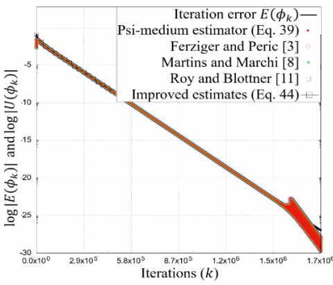
The modulus of iteration error $\left(E_k\right)$ and its estimates $\left(U_k\right)$ for all necessary iterations until machine error was reached in this case were computed and are represented in logarithmic scale (refer to the appendix - Figure 1A). Due to the extensive number of iterations, the analysis of estimates was performed post interval delimitation.
An analysis of the initial intervals revealed inaccuracies in the estimates, as corroborated by the estimator effectiveness (Eq. (28)), which stood at $64 \%$ for variable $T(1 / 2)$ and $22 \%$ for variable $T_m$.
It should be noted that in this model, the solver necessitates several iterations for the integration of boundary conditions into the calculations of local variables. However, the iteration count required to achieve machine error was lower compared to the previous model. Similar to Model 1, the presence of round-off error in Model 2 was also evident in the final iteration range for each variable, manifesting a graph behavior akin to that observed in Figure 5 of Model 1.
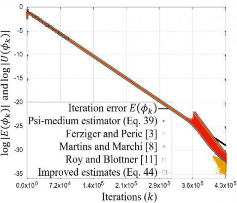
Model 3: The delimitation of iteration intervals was based on the criteria of $\psi$ 's monotonic convergence and the minimal impact of round-off errors. Table 6 summarizes these intervals. The optimal interval for variable $T(1/2, 1/2)$ was identified as Interval II, while for variables $\nabla T(1, y)$ and $T_m$, Interval III was deemed most effective.
The evaluation of the iteration error estimates across all iterations revealed a need for enhancement in the initial and final ranges. This observation is further illustrated in the appendix (Figure 2A), which presents the behavior of these estimates for Model 3.
In the first two models, variable $T(1 / 2)$ required the most effort in interval characterization due to its non-monotonic behavior of $\psi$, contrasting with variables $\nabla T(1)$ and $\left(T_m\right)$, where $\psi$ exhibited less variation. To refine the estimates, as proposed in the methodology, corrected numerical solutions were computed. The results of this corrective approach are discussed in the following subsection.
A comparison of the estimates reveals a similarity in the performance of the psi-medium estimator with those documented in the literature [3, 8, 11]. The methodology of this study aims to enhance these estimates by calculating corrected numerical solutions, the outcomes of which are detailed in the subsequent subsection.
Table 6. Delimited iteration intervals for psi-medium estimator analysis in Model 3 Case 2
|
Variable |
Interval |
Criteria |
Iterations |
|
$T\left(\frac{1}{2}, \frac{1}{2}\right)$ |
I |
$-1 \leq \psi \leq 1$ |
129 : 4526 |
|
II |
$\psi>1^1$ |
4527 : 60015 |
|
|
III |
$\psi>1^2$ |
60016 : 435850 |
|
|
$\nabla T(1, y)$ |
I |
$\psi>1$ |
3 : 18475 |
|
II |
$\psi>1^3$ |
18476 : 21076 |
|
|
III |
$\psi>1^1$ |
21077 : 92635 |
|
|
IV |
$\psi>1^2$ |
92636 : 440370 |
|
|
$T_m$ |
I |
$\psi>1$ |
3 : 15160 |
|
II |
$\psi>1^3$ |
15161 : 17764 |
|
|
III |
$\psi>1^1$ |
17765 : 87281 |
|
|
IV |
$\psi>1^2$ |
87282 : 429852 |
Notes: ¹monotonic convergence of $\psi$ without significant round-off errors; ²monotonic convergence of $\psi$ with significant round-off errors; ³no monotonic convergence of $\psi$.
5.3 Post-processing
This subsection delineates the post-processing of results as outlined in the methodology. Specifically, the solution corresponding to the last iteration of the best estimates interval ($\phi_{k_2}$) was deemed the most accurate. Subsequently, this solution was employed in Eq. (44) to compute enhanced estimates.
Model 1: Table 7 presents the solutions obtained at the final iteration of the optimal interval estimates for each case of Model 1.
Table 7. Solutions at the last iteration of optimal interval estimates for Model 1
|
Variable |
Case |
Iteration |
$\phi_{k_2}$ |
|
$T(1 / 2)$ |
1 |
2854 |
6.256103515625000E-02 |
|
2 |
36832 |
6.250381469726562E-02 |
|
|
3 |
457815 |
6.250023841857927E-02 |
|
|
$\nabla T(1)$ |
1 |
5480 |
3.997825622558593E+00 |
|
2 |
66428 |
3.999863028526306E+00 |
|
|
3 |
726608 |
3.999991422535594E+00 |
|
|
$T_m$ |
1 |
5470 |
2.001220583915710E-01 |
|
2 |
64392 |
2.000076293479651E-01 |
|
|
3 |
678463 |
2.000004768370261E-01 |
Utilizing these findings, solutions were recalculated across all intervals using Eq. (43), resulting in new solutions with diminished iteration errors. A marked improvement was observed in the initial phase of the iterative cycle upon comparing the numerical solutions.
Subsequent to the calculation of new estimates, results were systematically presented, aligned with the pre-defined intervals to facilitate enhanced visualization. For variable $T(1 / 2)$, intervals I, II, and III predominantly harbored less precise estimates as per the psi-medium estimator. As illustrated in Figure 6 (a), both the initial and recalculated estimates are depicted, revealing notable improvements in the accuracy of error predictions within these specific intervals. Analogous enhancements were also discernible for other variables of interest, as evidenced in Figures 6 (b) and 6 (c).
(a)
(b)
(c)
Figure 6. Comparison of original estimates, iteration error, and improved estimates for Model 1 Case 3
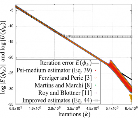
For variable $T(1 / 2)$, an initial divergence between the estimates and the iteration error was observed at the onset of interval IV. Subsequent recalculations of estimates, as detailed in the methodology, yielded significant improvements. This enhancement is depicted in Figure 7. The recalculated estimates exhibited higher accuracy compared to the initial estimates derived from the estimators. A similar trend of improved accuracy was noted in the other models, as illustrated in the appendix (Figures 3A and 4A).
Toward the terminal phase of each interval delineated for the respective variables, the pronounced emergence of round-off errors precluded the full alignment of all estimates. This limitation is exemplified in Figure 8, particularly in Figure 8 (a), where recalculated estimates begin to deviate from the actual iteration error around the iteration of order $3.6 \times 10^6$. Analogous patterns are observable in Figures 8 (b) and 8 (c), underscoring a consistent trend across the variables.
Figure 7. Enhanced estimate alignment for variable $T(1 / 2)$ in Model 1 Case 3.
Despite these challenges, the recalculated estimates in earlier intervals closely matched the true iteration error, surpassing the accuracy of initial estimates. However, for the ultimate interval, reliance solely on the estimator is recommended. The corrective solution procedure proved insufficient in mitigating the impact of round-off errors in this final stage. Figure 9 introduces the hybrid procedure, amalgamating the two estimation methodologies. In Figure 9(a), for instance, the corrected solution is applied in intervals I to IV, while only the estimator is utilized in interval V. This hybrid approach, as depicted in Figures 9(b) and 9(c), represents an optimized strategy for estimating iteration errors throughout the entire iterative process.
(a)
(b)
(c)
Figure 8. Estimates, iteration error and improved estimates for variables in Model 1 Case 3
(a)
(b)
(c)
Figure 9. Hybrid procedure for variables in Model 1 Case 3
Model 2: The recalculated solutions for all intervals, utilizing the numerical solution $\phi_{k_2}$ indicated in Table 8, demonstrated substantial improvements, particularly in the initial iterations.
Table 8. Final iteration solutions for all cases
|
Variable |
Case |
Iteration |
$\phi_{k_2}$ |
|
$T(1 / 2)$ |
1 |
2226 |
6.625315389083413E-03 |
|
2 |
28800 |
6.688624561987254E-03 |
|
|
3 |
354533 |
6.692586755646682E-03 |
|
|
$\nabla T(1)$ |
1 |
3353 |
9.947932529721088E+00 |
|
2 |
40567 |
9.996783336138475E+00 |
|
|
3 |
441845 |
1.000021786589429E+01 |
|
|
$T_m$ |
1 |
3489 |
9.995551575164478E-02 |
|
2 |
43358 |
9.995465571973533E-02 |
|
|
3 |
492493 |
9.995460161728745E-02 |
(a)
(b)
(c)
Figure 10. Hybrid Procedure Implementation for variables in Model 2 Case 3
Utilizing these solutions, new estimates were calculated. However, similar to previous models, the final iteration intervals for variables $T(1 / 2)$ (Interval III), and $\nabla T$ and $T_m$ (Interval II) did not exhibit marked improvements due to the presence of round-off errors. Therefore, the corrected solution approach is advised for recalculating estimates in intervals minimally affected by round-off errors. For other intervals, the psi-medium estimator is recommended (Figure 10).
Model 3: The application of the hybrid procedure in Model 3 is presented through the analysis of solutions with reduced iteration errors, as summarized in Table 9.
Table 9. Last iteration Solutions for variables for all cases
|
Variable |
Case |
Iteration |
$\phi_{k_2}$ |
|
$T(1 / 2)$ |
1 |
4738 |
1.993260416376170E-01 |
|
2 |
60015 |
1.992720104130132E-01 |
|
|
$\nabla T(1)$ |
1 |
8041 |
9.282659951979760E-01 |
|
2 |
92635 |
9.197616756887540E-01 |
|
|
$T_m$ |
1 |
7826 |
1.809084632456606E-01 |
|
2 |
87281 |
1.846122358980575E-01 |
The recalculated estimates, derived using Eq. (44), exhibited notable improvements in accuracy during the initial intervals of the iterative process. This advancement is particularly evident in the early stages of the iterative cycle, showcasing the efficacy of the new estimates.
Nonetheless, similar to the challenges encountered with previous models, the final interval of Model 3 did not show any substantial enhancement in estimates due to the prevalence of round-off errors. Consequently, it is advised to employ the corrected solutions for estimate calculation in the early intervals and utilize the psi-medium estimator for the latter interval. This approach is encapsulated in Figure 11, which illustrates the implementation of the hybrid estimation method.
(a)
(b)
(c)
Figure 11. Application of the hybrid procedure for variables in Model 3 Case 2
In this research, rigorous techniques were employed to verify computational codes, involving grid refinement and juxtaposition of numerical solutions against analytical counterparts. Analyses, both a priori and a posteriori, were conducted to assess the decay order of discretization errors. It was observed that the effective and apparent equivalent orders invariably aligned with the asymptotic orders of the numerical schemes utilized, fulfilling the initial objectives of this study. This accomplishment paved the way for subsequent phases.
The initial estimates, derived using the psi-medium estimator, exhibited a close resemblance to those reported in extant literature [3, 8, 11]. In pursuit of enhancing these estimates, iteration intervals for each variable of interest were meticulously delineated. The criteria for this delineation hinged on the values of the convergence rate ψ and the impact of round-off errors.
Across all variables, the optimal range for estimates was identified as the interval characterized by a monotonic convergence of ψ and minimal influence from round-off errors. Subsequently, a novel procedure was implemented to reduce iteration errors, leading to the calculation of corrected solutions. The final corrected solution within the most favorable interval, deemed as the most precise, was utilized for recalculating the estimates.
The re-evaluated estimates exhibited a marked enhancement in the accuracy of iteration error predictions across all defined intervals for each variable under study. This improvement was noted in contrast to earlier obtained estimates, with the exception of the final interval. The precision of these new estimates was found to be contingent upon the accuracy of the corrected solutions used for their calculation, and was also affected by the presence of round-off errors. To address this limitation, two strategies were proposed: firstly, selecting the iteration that yielded the minimum value in the difference calculated by Eq. (41), and secondly, applying the empirical psi-medium estimator as a post-processing tool on the obtained numerical solutions.
Consequently, it was discerned that a hybrid procedure, integrating the use of corrected solutions to enhance estimates in the initial intervals, combined with the exclusive application of the psi-medium estimator in the terminal intervals, offered a distinct advantage. This approach notably surpassed the performance of other estimators, particularly in the early phases of the iterative cycle. The study's final objectives were thus fulfilled, underscoring the efficacy of monitoring the convergence rate ψ as a means to facilitate a more comprehensive analysis of the iterative cycle's intervals, ultimately leading to more accurate estimation outcomes.
In the realm of CFD, the finite volume method predominates for discretizing model equations. However, in the initial phase of this research, the FDM was selected. Future endeavors will incorporate a diverse array of discretization techniques, alongside varying solvers, including the modified strongly implicit procedure (MSI), both with and without the integration of multigrid methods, to rigorously evaluate the methodology.
The enhancement of the hybrid procedure will involve the application of mathematical models featuring coupled equations. Notably, the study plans to engage with the two-dimensional Burgers and Navier-Stokes equations, employing a range of Reynolds numbers. Furthermore, efforts will be directed toward computing iteration error estimates across the complete spectrum of the numerical solution field. The overarching goal remains steadfast: to refine the accuracy of these estimates and achieve a reduction in iteration error.
This work was supported by the National Council for Scientific and Technological Development (CNPq), the Graduate Program in Mechanical Engineering (PG-Mec) from the Federal University of Paraná (UFPR) and the Federal University of Technology - Paraná (UTFPR). The Laboratory of Numerical Experimentation (LENA) provided the network infrastructure. The second author was scholarship of CNPq. This study was financed in part by the Coordenação de Aperfeiçoamento de Pessoal de Nível Superior - Brasil (CAPES) - Finance Code 001.
|
$a_n^T$ |
coefficients of the discretized equation system of the mathematical model |
|
$b^T$ |
source term of the discretized equation system of the mathematical model |
|
c |
coefficients that depend on $\Phi$ and do not depend on h |
|
$E\left(\phi_k\right)$ |
iteration error in the current iteration $k$ |
|
$U\left(\phi_k\right)$ |
estimate of iteration error in the current iteration $k$ |
|
$E_\pi$ |
round-off error |
|
$E_h$ |
discretization error |
|
$E_k$ |
iteration error |
|
$E_n$ |
numerical error |
|
h |
grid step size |
|
k |
iteration number |
|
$l^2$ |
$z_k / z_{k+1}$ |
|
$L$ |
domain length |
|
$N$ |
number of grid points |
|
$P e$ |
Péclet number |
|
$p_0$ |
asymptotic order decay of iteration error |
|
$p_{E_h}^*$ |
effective equivalent order of discretization error |
|
$p_U$ |
apparent order of estimates |
|
$p_{U_h}^*$ |
apparent equivalent order of discretization error |
|
$r$ |
grid refinement ratio |
|
$r_e$ |
$\left|z_k\right| /\left|\chi_{k_2}\right|$ |
|
$T$ |
continuous function that represents the exact analytical solution of the dependent variable |
|
$T^{(n)}$ |
n-th derivative of the exact analytical solution |
|
$T_m$ |
exact analytical solution of the mean value of T |
|
$x$ |
independent variable’s continuous function |
|
$y$ |
independent variable’s continuous function |
|
$Z$ |
$\chi_{k-2} \cdot \chi_k-\chi_{k-1} \cdot \chi_{k-1}$ |
|
Greek symbols |
|
|
$\alpha$ |
Constant |
|
$\beta$ |
Constant |
|
$\lambda_1$ |
dominant eigenvalue |
|
$\Phi_a$ |
analytical solution of a variable of interest |
|
$\phi$ |
numerical approximation of a variable of interest |
|
$\Omega$ |
calculation domain |
|
$\psi$ |
convergence rate |
|
$\theta$ |
estimates effectiveness |
|
$\nabla$ |
Gradient |
|
Subscripts |
|
|
$a$ |
analytical solution |
|
$i$ |
reference grid point on $x$ direction |
|
$j$ |
reference grid point on $y$ direction |
|
$k$ |
current iteration |
|
$k_1$ |
first iteration of the best interval estimates |
|
$k_2$ |
last iteration of the best interval estimates |
|
$m$ |
mean value |
|
$x$ |
$x$ direction |
|
$y$ |
$y$ direction |
|
$\infty$ |
converged/estimated solution |
(a)
(b)
(c)
Figure 1A. Estimates and iteration error at each iteration for the variables $T(1 / 2)(\mathrm{a}), \nabla T(1)$ (b) and $T_m$ (c), of model 2, case 3, in all iterations
(a)
(b)
(c)
Figure 2A. Estimates and iteration error at each iteration for the variables $T(1 / 2,1 / 2)(\mathrm{a}), \nabla T(1, y)(\mathrm{b})$ and $T_m$ (c), of model 3, case 2
(a)
(b)
(c)
Figure 3A. Estimates, iteration error and improved estimates at each iteration for the variables $T(1 / 2)$ in the intervals I and II (a); $\nabla T(1)$ in the interval I; and $T_m$ of model 2, case 3, in the interval I.
(a)
(b)
(c)
Figure 4A. Estimates, iteration error and improved estimates at each iteration for the variables $T(1 / 2,1 / 2)$ in the intervals I (a); $\nabla T(1, y)$ in the interval I and II; and $T_m$ of model 3, case 2, in the interval I and II
[1] Fortuna, A.O. (2000). Computational techniques for fluid dynamics (in Portuguese). University of São Paulo Press.
[2] Pereira, F., Eça, L., Vaz, G. (2017). Verification and validation exercises for the flow around the KVLCC2 tanker at model and full-scale Reynolds numbers. Ocean Engineering, 129: 133-148. http://doi.org/10.1016/j.oceaneng.2016.11.005
[3] Ferziger, J.H., Peric, M. (1996). Further discussion of numerical errors in CFD. International Journal for Numerical Methods in Engineering, 23: 1263-1274. http://doi.org/10.1002/(SICI)1097-0363(19961230)23:12%3C1263::AID-FLD478%3E3.0.CO;2-V
[4] Roache, P.J. (2009). Fundamentals of Verification and Validation. Hermosa Publishers.
[5] Eça, L., Vaz, G., Hoekstra, M., Pal, S., Muller, E., Pelletier, D., Bertinetti, A., Difonzo, R., Savoldi, L., Zanino, R., Zappatore, A., Chen, Y., Maki, K. J., Ye, H., Drofelnik, J., Moss, B., Da Ronch, A. (2020). Overview of the 2018 workshop on iterative errors in unsteady flow simulations. ASME. Journal of Verification, Validation and Uncertainty Quantification, 5(2): 021006. http://doi.org/10.1115/1.4047922
[6] Eça, L., Hoekstra, M. (2006). On the influence of the iterative error in the numerical uncertainty of ship viscous flow calculations. In 26th Symposium on Naval Hydrodynamics, Rome, Italy.
[7] Eça, L., Vaz, G., Hoekstra, M. (2017). Iterative errors in unsteady flow simulations: Are they really negligible? In Proceedings of the 20th Numerical Towing Tank Symposium, Wageningen, the Netherlands.
[8] Martins, M.A., Marchi, C.H. (2008). Estimate of iteration errors in CFD. Numerical Heat Transfer, Part B: Fundamentals, 53(3): 234-245. http://doi.org/10.1080/10580530701790142
[9] ASME. (2009). Standard for verification and validation in CFD and heat transfer, V V 20 - 2009(R2021).
[10] Ferziger, J.H., Peric, M., Street, R.L. (2012). Computational Methods for Fluid Dynamics. Springer Science & Business Media. http://doi.org/10.1007/978-3-319-99693-6
[11] Roy, C.J., Blottner, F.G. (2001). Assessment of one-and two-equation turbulence models for hypersonic transitional flows. Journal of Spacecraft and Rockets, 38(5): 699-710. http://doi.org/10.2514/6.2001-210
[12] Payne, J.L., Hassan, B. (1998). Massively parallel CFD calculations for aerodynamics and aerothermodynamics applications. Technical report, Sandia National Labs., Aerosciences and Compressible Fluid Mechanics Dept., Albuquerque, NM (United States).
[13] Incropera, F.P., Lavine, A.S., IncroperaDe, F.P., Witt, D.P. (1998). Fundamentals of Heat and Mass Transfer. John Wiley & Sons, Inc.
[14] Tannehill, J.C., Anderson, D., Pletcher, R.H. (1997). Computational Fluid Mechanics and Heat Transfer. Washinton, DC: Taylor & Francis. https://doi.org/10.1201/9781351124027
[15] Kreyszig, E. (2010). Advanced Engineering Mathematics. New York: John Wiley & Sons.
[16] Chapra, S.C., Canale, R.P. (2008). Numerical Methods for Engineering. São Paulo: McGraw-Hill.
[17] Burden, R., Faires, J. (2011). Numerical Analysis. Boston: Cengage Learning.
[18] Atkinson, K.E. (1967). The numerical solution of the fredhom integral equations of the second kind. SIAM Journal on Numerical Analysis, 4(3): 337-348.
[19] Cunha, M.C.C. (2000). Numerical Methods. Unicamp Press. https://repositorio.unicamp.br/acervo/detalhe/796274.
[20] Maliska, C.R. (2010). Heat Transfer and Computational Fluid Mechanics. LTC Editora, Rio de Janeiro.
[21] Moro, D.F. (2018). Developing techniques to reduce iteration and discretization errors in CFD (in Portuguese). Ph.D. thesis. Department of Mechanical Engineering, Federal University of Paraná, Curitiba, Brazil.
[22] Moro, D.F., Marchi, C.H., Pinto, M.A.V. (2015). An efficient interactive method for solving systems of pentadiagonal equations. Proceeding Series of the Brazilian Society of Computational and Applied Mathematics, 3(2): 020078. https://doi.org/10.5540/03.2015.003.02.0078
[23] Marchi, C.H. (2001). Verification of one-dimensional numerical solutions in fluid dynamics (in Portuguese). Ph.D. thesis. Department of Mechanical Engineering, Federal University of Santa Catarina, Florianópolis, Brazil.
[24] da Silva, L., Marchi, C., Meneguette, M., Foltran, A. (2022). Robust RRE technique for increasing the order of accuracy of SPH numerical solutions. Mathematics and Computers in Simulation, 199: 231-252. http://doi.org/10.1016/j.matcom.2022.03.016
[25] Roy, C.J., Oberkampf, W.L. (2011). A comprehensive framework for verification, validation, and uncertainty quantification in scientific computing. Computer Methods in Applied Mechanics and Engineering, 200(25): 2131-2144. http://doi.org/10.1016/j.cma.2011.03.016
[26] da Silva, L.P., Meneguete Junior, M., Marchi C.H. (2023) Numerical Error Analysis and Heat Diffusion Models. pp 51-75. Springer, Cham. https://doi.org/10.1007/978-3-031-28946-0_3
[27] da Silva L.P., Rutyna, B.B., Righi, A.R.S., Pinto M.A.V. (2021) High order of accuracy of Poisson equation obtained by grouping of repeated Richardson extrapolation with fourth order schemes. Computer Modeling in Engineering & Sciences, 128(2): 669-715. http://doi.org/10.32604/cmes.2021.014239
[28] Marchi, C.H., Novak, L.A., Santiago, C.D., da Silveira Vargas, A.P. (2013). Highly accurate numerical solutions with repeated Richardson extrapolation for 2D Laplace equation. Applied Mathematical Modelling, 37(12-13): 7386-7397. http://doi.org/10.1016/j.apm.2013.02.043
[29] Shyy, W., Garbey, M., Appukuttan, A., Wu, J. (2002). Evaluation of Richardson extrapolation in CFD. Numerical Heat Transfer: Part B: Fundamentals, 41(2): 139-164. http://doi.org/10.1080/104077902317240058
[30] Jézéquel, F., Chesneaux, J. M. (2008). CADNA: A library for estimating round-off error propagation. Computer Physics Communications, 178(12): 933-955. http://doi.org/10.1016/j.cpc.2008.02.003
[31] Kaneko, T., Liu, B. (1970). Accumulation of round-off error in fast Fourier transforms. Journal of the ACM (JACM), 17(4): 637-654. http://doi.org/10.1145/321607.321613
[32] Moro, D.F., Marchi, C.H. (2017). Efeito de hardware e software sobre o erro de arredondamento em CFD. Proceeding Series of the Brazilian Society of Computational and Applied Mathematics, 5(1): http://doi.org/10.5540/03.2017.005.01.0315
[33] Zhu, J.Z., Zienkiewicz, O.C. (1990). Super convergence recovery technique and a posteriori error estimators. International Journal for Numerical Methods in Engineering, 30: 1321-1339. http://doi.org/10.1002/nme.1620300707