Ahmed A. Mohammed Fawze*![]() | Anees Abdallah Fthee
| Anees Abdallah Fthee![]()
© 2024 The authors. This article is published by IIETA and is licensed under the CC BY 4.0 license (http://creativecommons.org/licenses/by/4.0/).
OPEN ACCESS
Problems exhibiting wave-like characteristics pervade a diverse array of physical phenomena, including but not limited to longitudinal vibrations of elastic rods or beams, acoustic problems in fluid flow, electric signal transmission along cables, shock waves, chemical exchange processes in chromatography, sediment transport in rivers, plasma wave behavior, and the propagation of both electric and magnetic fields in the absence of charge and dielectric. This study introduces a novel series solution for wave-like problems, leveraging a newly developed technique within the Homotopy Perturbation Method (HPM). The proposed technique operates in the absence of a need for discretization, linearization, or restrictive assumptions, offering distinct advantages over conventional methods. This new version of HPM is designed to address wave-like problems. The technique rests on the assumption that the required solution can be represented as an infinite series sum. The proposed series demonstrates rapid convergence through the use of a control parameter. Initially, the parameter's scope is determined, followed by the selection of a single value that facilitates convergence. Various examples were applied using this technique, yielding satisfactory results. The novel version of HPM presented in this study hinges on the concept of representing the solution as an infinite series sum. This approach exhibits rapid convergence to the precise solution, enabled by the use of a control parameter. The parameter region is initially determined, followed by the selection of a single value that ensures convergence with a satisfactory sum count.
wave equations, Fredholm integral equation, Homotopy Perturbation Method (HPM)
Wave-like problems, which describe the propagation of a wave or disturbance, are a fundamental aspect of various physical systems. These disturbances are not limited to a particular domain but permeate a plethora of physical phenomena, thereby establishing their universal relevance. The list of physical systems influenced by wave-like problems includes the vibrations of strings and membranes, longitudinal vibrations of elastic rods or beams, acoustic problems concerning the velocity potential for sound-transmitting fluid flow, and electric signal transmission along cables. Even more complex scenarios, such as shock waves, chemical exchange processes in chromatography, sediment transport in rivers, wave phenomena in plasmas, and the propagation of both electric and magnetic fields in the absence of charge and dielectrics, can be modeled using wave-like equations [1, 2].
In the realm of applied mathematics, wave-like problems are often articulated using nonlinear second order wave partial differential equations (WPDEs). These WPDEs have been instrumental in describing the progression of waves, as exhibited in the vibration of strings and membranes. Therefore, an effective methodology to solve these equations is crucial for advancing our understanding of these physical phenomena.
The Homotopy Perturbation Method (HPM) emerges as a specialized approach in this context, demonstrating its effectiveness in treating Partial Integral Equations (PIEs) of various types and kinds [3]. The versatility of the HPM is underscored by its successful application to a diverse set of problems, such as systems of nonlinear coupled equations [4], nonlinear Volterra-Hammerstein integral equations [5-7], singular Volterra integral equations of the first kind [8, 9], singular integro-differential equations [10], stochastic partial differential equations [11], and a specific type of Volterra integral equations in two-dimensional space [12].
Moreover, modifications to the HPM have proven to be fruitful in obtaining exact solutions for Nonlinear Integral Equations (NIE) [13]. A novel Inverse Iterative Numerical Scheme (IINS) is used to examine Eigen functions in mathematical treatment of 2nd-order Fredholm integral problems a partial differential equation solution technique [14]. It uses Homotopy perturbation theory, a well-known approach [15]. In this research, we aim to extend the utility of the HPM by introducing a novel technique that focuses on solving wave-like problems. This technique operates without the requirement for discretization or linearization, eliminating the need for restrictive assumptions that often limit the applicability of other methods. This new version of the HPM, designed specifically to address wave-like problems, is predicated on the assumption that the required solution can be represented as an infinite series sum. Importantly, the convergence of the series is expedited through the use of a control parameter. The parameter scope is initially determined, and then a single value is selected to facilitate rapid convergence.
A series of examples are provided to validate the efficacy of this method. These examples have been carefully chosen to represent a diverse set of wave-like problems, and the results obtained from our method are compared with existing solutions to verify the accuracy and speed of convergence. The outcomes are promising, showcasing the potential of this novel method in dealing with complex wave-like problems.
The structure of this paper aims to provide a comprehensive journey through the development and application of this new method. Following this introduction, the paper presents the motivation behind this research, explaining the need for such a method in the context of wave-like problems. Thereafter, the mathematical manipulation and solution strategy are detailed, offering a deep dive into the workings of the method. This is followed by numerical results obtained from various test cases, providing quantitative evidence of the method's effectiveness. The discussion section then elaborates on these results, providing insights and potential implications. The paper concludes with a summary of the research and potential future directions. Finally, references are provided to allow readers to delve deeper into the concepts discussed.
1.1 Research motivation
The present paper, is a trial to present new version of the series method based Homotopy perturbation techniques. As far we know from our search in the Homotopy perturbation used by different ways, so in our paper, we try to make good connection between series and Homotopy perturbation.
1.2 Mathematical manipulation
Consider the following non-linear, 2ndorder, 1-D wave equation:
$\frac{\partial^2 T(x, t)}{\partial t^2}=\mathfrak{I}(T) \frac{\partial^2 T(x, t)}{\partial x^2}+\frac{\partial \mathfrak{I}(T)}{\partial x} \frac{\partial T(x, t)}{\partial x}$ (1)
in which:
$\Im(T)=(T(x, t))^2$ (2)
According to HPM, we can construct a Homotopy $v(\mathrm{r} ; \zeta): \Omega \times[0,1] \rightarrow \Re$ and the domain Ω satisfies:
$H(\mathrm{r} ; \zeta)=(1-\zeta) F(v)+p \ell(v)=0$ (3)
The term F(ν) is known as FO with known solution T0, which can be obtained easily, clearly, we have:
$H(\mathrm{v} ; 0)=F(v)$ (4)
$H(\mathrm{v} ; 1)=\ell(v)$ (5)
Applying the Homotopy axioms, and let us construct the zero order deformation as follows:
$(1-\zeta) \ell\left[\varpi(r, t, \zeta)-T_0(r, t)\right]=\zeta \hbar H(r, t) N(r, t, \zeta)$ (6)
In Eq. (2):
ζ: Parameter $\in$[0,1]
$\ell$: Linearoperator
$\hbar$: Auxiliary parameter
T0(r, t): Initial solution
T(x, t): Exact or approximate required solution
$\varpi(r, t, \zeta)$: Unknown auxiliary function
The linear operator has the following properties:
$\varpi(r, t, 0)=T_0(r, t)$ (7)
$\varpi(r, t, 1)=T(r, t)$ (8)
The next step is to expand $\varpi(r, t, \zeta)$ in its Taylor’s expansion as follows:
$\varpi(r, t, \zeta)=T_0(r, t)+\sum_{j=1}^{j \rightarrow \infty} T_j(r, t) \zeta^m$ (9)
In Eq. (9):
$T_j(r, t)=\left.\frac{1}{j !} \frac{\partial^j \varpi(r, t, \zeta)}{\partial \zeta^m}\right|_{\zeta=0}$ (10)
Substituting from Eq. (10) into Eq. (9), the later becomes:
$\varpi(r, t, \zeta)=T_0(r, t)+\sum_{j=1}^{j \rightarrow \infty}\left(\left.\frac{1}{j !} \frac{\partial^j \varpi(r, t, \zeta)}{\partial \zeta^m}\right|_{\zeta=0}\right) \zeta^m$ (11)
The series in Eq. (11), is convergent at ζ=1.
Eq. (11) at ζ=1 takes the following form:
$T(r, t)=T_0(r, t)+\sum_{j=1}^{j \rightarrow \infty} T_j(r, t)$ (12)
Eq. (12), should be one of the solutions of N(r, t)=0
The next step is to find j-derivatives for Eq. (6), i.e., we need to find the following derivatives:
$\frac{\partial}{\partial \zeta}\left\{(1-\zeta) \ell\left[\varpi(r, t, \zeta)-T_0(r, t)\right]\right\}=\frac{\partial}{\partial \zeta}\{\zeta \hbar H(r, t) N(r, t, \zeta)\}$ (13)
$\begin{gathered}\frac{\partial^2}{\partial \zeta^2}\left\{(1-\zeta) \ell\left[\varpi(r, t, \zeta)-T_0(r, t)\right]\right\}= \frac{\partial^2}{\partial \zeta^2}\{\zeta \hbar H(r, t) N(r, t, \zeta)\}\end{gathered}$ (14)
$\frac{\partial^3}{\partial \zeta^3}\left\{(1-\zeta) \ell\left[\varpi(r, t, \zeta)-T_0(r, t)\right]\right\}=\frac{\partial^3}{\partial \zeta^3}\{\zeta \hbar H(r, t) N(r, t, \zeta)\}$
$\frac{\partial^j}{\partial \zeta^j}\left\{(1-\zeta) \ell\left[\varpi(r, t, \zeta)-T_0(r, t)\right]\right\}=\frac{\partial^j}{\partial \zeta^j}\{\zeta \hbar H(r, t) N(r, t, \zeta)\}$ (15)
Next, each equation from (13) to (15) is then divided by ζ!, then last put all at ζ=0, after mathematical manipulations and simplifications, one can get the jth -order deformation equation:
$\begin{gathered}L\left\{T_j(r, t)-\varsigma_j T_{\mathrm{j}-1}(r, t)\right\}=\frac{1}{(j-1) !}\left\{\hbar H(r, t) \frac{\partial^{j-1} \varpi(r, t, \zeta)}{\partial \zeta^{j-1}}\right\}_{\zeta=0}\end{gathered}$ (16)
Eq. (16) is in linear form and according to the Homotopy procedure, then it could be transformed to system of linear equations. The latter system will be solved using any iterative method. In the next section, some numerical examples with illustrative procedure will be solved.
The main criteria of the solution strategy is that how can we control the convergence behavior is the determination the optimal value for the control parameter $\hbar$ and the later can be determined according to the following procedure:
Step (1): Evaluate $\left.\frac{\partial T(x, t)}{\partial x}\right\}_{x=1, t=1}$
Step (2): Evaluate $\left.\frac{\partial^2 T(x, t)}{\partial t^2}\right\}_{x=1, t=1}$
Step (3): Plot the above two derivatives, and the rejoin between the two curves leads to the interval of convergence for the control parameter
Step (4): Take the average value for the control parameter
2.1 Flow chart for solution procedure
In this part, we will write in detail the explanation of the method in the form of a flow chart in Figure 1.
Figure 1. Flow chart for solution procedure
2.2 Numerical results
To test the proposed method, two different examples are solved, non-linear, 2nd order partial differential equation, followed by a third one is non-Linear, 2nd order, 1-D Wave Equation as shown in Figures 2-4.
Test problem (1)
Solve the following non-linear, 2nd order partial differential equation, given by:
$\frac{\partial^2 T(x, t)}{\partial t^2}=\frac{\partial}{\partial x}\left(\frac{1}{T(x, t)}\left(\frac{\partial T(x, t)}{\partial x}\right)\right)$ (17)
Eq. (17) will be subjected to the following conditions:
$\begin{gathered}T_0(x, t)=T(x, t=0)=(1+x)^{-2} \\ \frac{\partial T(x, t=0)}{\partial t}=0\end{gathered}$ (18)
The jth -order deformation equation corresponding to Eq. (17), takes the following form:
$\begin{gathered}L\left\{T_j(r, t)-\varsigma_j T_{\mathrm{j}-1}(r, t)\right\}= \frac{1}{(j-1) !}\left\{\hbar H(r, t) \frac{\partial^{j-1} \varpi(r, t, \zeta)}{\partial \zeta^{j-1}}\right\}_{\zeta=0}\end{gathered}$ (19)
According to the concept of the jth-order deformation equation, the conditions given in Eq. (18), takes the following form:
$\begin{aligned} & T_j(x, 0)=0 \\ & \frac{\partial T_j(x, 0)}{\partial t}=0\end{aligned}$ (20)
Therefore, one can get the following:
$\begin{gathered}T_1(x, t)=\hbar t^2(1+x)^{-2} \\ T_2(x, t)=-\hbar(1+\hbar) t^2(1+x)^{-2} \\ T_3(x, t)=-\hbar(1+\hbar)^2 t^2(1+x)^{-2} \\ \cdots \\ T_n(x, t)=-\hbar(1+\hbar) t^{\mathrm{n}-1}(1+x)^{-2}\end{gathered}$ (21)
Therefore, the series solution takes the following form:
$\begin{gathered}T(x, t)=(1+x)^{-2}\left(1-\hbar t^{\mathrm{n}-1} \sum_{n=1}^{\infty}(1+\hbar)^{n-1}\right), |1+\hbar|<1\end{gathered}$ (22)
Figure 2. Results graph due to the present method
Test problem (2)
Solve the following non-linear, 2nd order partial differential equation, given by:
$\frac{\partial^2 T(x, t)}{\partial t^2}=\frac{\partial}{\partial x}\left(T^{-2}(x, t) \frac{\partial^2 T(x, t)}{\partial x^2}\right)$ (23)
Eq. (29) will be subjected to the following conditions:
$\begin{aligned} & T_0(x, t)=x \\ & \frac{\partial T(x, 0)}{\partial t}=-x\end{aligned}$ (24)
The jth -order deformation equation, takes the following form:
$\begin{gathered}L\left\{T_j(r, t)-\varsigma_j T_{\mathrm{j}-1}(r, t)\right\}=\frac{1}{(j-1) !}\left\{\hbar H(r, t) \frac{\partial^{j-1} \varpi(r, t, \zeta)}{\partial \zeta^{j-1}}\right\}_{\zeta=0}\end{gathered}$ (25)
According to the concept of the jth-order deformation equation, the conditions given in Eq. (18), takes the following form:
$\begin{aligned} & T_j(x, 0)=0 \\ & \frac{\partial T_j(x, 0)}{\partial t}=0\end{aligned}$ (26)
Let us choose the initial starts as follows:
$T_0(x, t)=x(1-t)$
Therefore; one can get the following:
$\begin{aligned} & T_1(x, t)=0.1 \times \hbar \times t^2\left[-10+10 \mathrm{t}-5 \mathrm{t}^2+t^3\right] \times x \\ & T_2(x, t)=0.1 \times \hbar \times t^2\left[-10+10 \mathrm{t}-5 \mathrm{t}^2+t^3\right] \times x \\ & -120^{-1} \hbar^2 \times t^2\left[-120+120 \mathrm{t}+96 \mathrm{t}^3-84 \mathrm{t}^4+36 t^5-9 t^6+t^7\right]\end{aligned}$ (27)
Therefore, the series solution for 10 terms as an approximation takes the following form:
$T(x, t)=x(1-t)+\left(\sum_{n=1}^{10} T_n(x, t)\right)$ (28)
Figure 3. Abs. Error between present and analytical at time 0.15
Figure 4. Abs. Error between present and analytical at time 0.15
Table 1. Computations due to the present method
|
x |
t=0.15 |
t=0.30 |
t=0.45 |
t=0.60 |
t=0.75 |
t=0.9 |
t=1.00 |
|
0.00 |
1.02255 |
1.09 |
1.2025 |
1.36 |
1.5625 |
1.81 |
2 |
|
0.25 |
0.6544 |
0.6976 |
0.7696 |
0.8704 |
1.0000 |
1.1584 |
1.28 |
|
0.50 |
0.4544 |
0.4844 |
0.9344 |
1.1378 |
1.3611 |
1.6044 |
1.7778 |
|
0.75 |
0.4318 |
0.5518 |
0.6865 |
0.8359 |
1.0000 |
1.1788 |
1.3061 |
|
1.0 |
0.3306 |
0.4225 |
0.5256 |
0.6400 |
0.7656 |
0.9025 |
1.0000 |
Table 2. Abs. error corresponding to $\hbar$=-1.111
|
|
Previous Results |
Present Results |
Previous Results |
Present Results |
Previous Results |
Present Results |
Previous Results |
Present Results |
|
X |
t = 0.5 |
t = 1.0 |
t = 1.5 |
t = 2.0 |
||||
|
-3 |
4.95136×10⁻¹⁰ |
4.94033×10⁻¹⁰ |
2.31086×10⁻⁶ |
2.31066×10⁻⁶ |
1.87496×10⁻³ |
1.87282×10⁻³ |
5.78147×10⁻⁵ |
5.78001×10⁻⁵ |
|
-2 |
3.30098×10⁻¹⁰ |
3.29998×10⁻¹⁰ |
1.54057×10⁻⁶ |
1.53937×10⁻⁶ |
1.24997×10⁻³ |
1.25001×10⁻³ |
3.85432×10⁻⁵ |
3.85002×10⁻⁵ |
|
-1 |
1.65049×10⁻¹⁰ |
1.65112×10⁻¹⁰ |
7.70287×10⁻⁷ |
7.69222×10⁻⁷ |
6.24986×10⁻³ |
6.24732×10⁻³ |
1.92716×10⁻⁵ |
1.92602×10⁻⁵ |
|
+1 |
1.65049×10⁻¹⁰ |
1.65112×10⁻¹⁰ |
7.70287×10⁻⁷ |
7.69222×10⁻⁷ |
6.24986×10⁻³ |
6.24732×10⁻³ |
1.92716×10⁻⁵ |
1.92602×10⁻⁵ |
|
+2 |
3.30098×10⁻¹⁰ |
3.29998×10⁻¹⁰ |
1.54057×10⁻⁶ |
1.53937×10⁻⁶ |
1.24997×10⁻³ |
1.25001×10⁻³ |
3.85432×10⁻⁵ |
3.85002×10⁻⁵ |
|
+3 |
4.95136×10⁻¹⁰ |
4.94033×10⁻¹⁰ |
2.31086×10⁻⁶ |
2.31066×10⁻⁶ |
1.87496×10⁻³ |
1.87282×10⁻³ |
5.78147×10⁻⁵ |
5.78001×10⁻⁵ |
|
+4 |
6.60195×10⁻¹⁰ |
6.60084×10⁻¹⁰ |
3.08115×10⁻⁶ |
3.08005×10⁻⁶ |
2.49995×10⁻³ |
2.50001×10⁻³ |
7.70863×10⁻⁵ |
7.70001×10⁻⁵ |
Table 3. Minimum error
|
|
0.1 |
0.2 |
0.3 |
0.4 |
0.5 |
0.6 |
0.7 |
|
0.1 |
9×10⁻⁶ |
9×10⁻⁶ |
9×10⁻⁶ |
9×10⁻⁶ |
9×10⁻⁶ |
9×10⁻⁶ |
9×10⁻⁶ |
|
0.2 |
1.4×10⁻⁴ |
1.5×10⁻⁴ |
1.49×10⁻⁴ |
1.49×10⁻⁴ |
1.5×10⁻⁴ |
1.4×10⁻⁴ |
1.49×10⁻⁴ |
|
0.3 |
2×10⁻³ |
2.7×10⁻³ |
2.69×10⁻³ |
2.7×10⁻³ |
2.7×10⁻³ |
2.69×10⁻³ |
2.7×10⁻³ |
|
0.4 |
4.7×10⁻³ |
6.8×10⁻³ |
6.77×10⁻³ |
6.8×10⁻³ |
6.77×10⁻³ |
6.77×10⁻³ |
6.8×10⁻³ |
|
0.5 |
1.7×10⁻² |
2.6×10⁻² |
2.58×10⁻² |
1.7×10⁻² |
2.6×10⁻² |
1.7×10⁻² |
2.58×10⁻² |
|
0.6 |
2.9×10⁻² |
4.6×10⁻² |
4.55×10⁻² |
2.9×10⁻² |
4.6×10⁻² |
4.6×10⁻² |
4.55×10⁻² |
|
0.7 |
4.6×10⁻² |
7.5×10⁻² |
7.47×10⁻² |
7.5×10⁻² |
7.47×10⁻² |
7.5×10⁻² |
4.6×10⁻² |
Test problem (3)
Non-Linear, 2nd order, 1-D Wave Equation
Consider 1-D, wave equation with the following boundary and initial conditions:
$\frac{\partial^2 T(x, t)}{\partial t^2}-x^2 \frac{\partial^2 T(x, t)}{\partial x^2}=x \exp (t)-\left(\frac{\partial T(x, t)}{\partial x}\right)^2+\exp (2 t)$
Subject to
$\begin{gathered}T(x, 0)=x \\ \left\{\frac{\partial T(x, t)}{\partial t}\right\}_{t=0}=x \\ T(0, t)=0\end{gathered}$
The exact solution T(x, t)=x exp(t).
Tables 1-3 show the minimum error between the results due to the present method and the exact solution at different points of spatial variable x (Horizontal first raw) and different times (Vertical left column).
2.3 Importance of the problem in practice and the new of the proposed method
The paper introduces new hybrid technique to solve wide range of practical problems that can be found in different fields of science, engineering, and industry.
The main difference appear in the present method is that the simplicity in sequence and how to control the control parameter by knowing its interval then we can move in very small one so as we encounter better convergence as shown in Figures 5-6.
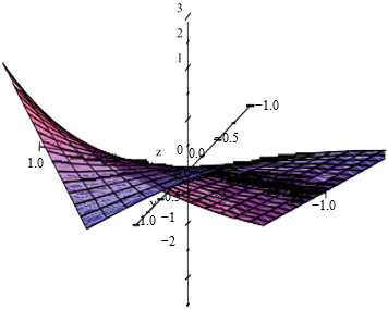
Figure 5. The exact solution
Figure 6. The approximate solution
This study undertook the resolution of two distinct examples utilizing the method proposed herein, and subsequently juxtaposed the results with pre-existing analytical and approximate solutions for comparison. The methodology for each example began with the determination of the convergence zone for the control parameter. Subsequently, a unique value within this zone was selected, which facilitated the derivation of the corresponding solution. Upon review of the results, it can be observed that the present solutions align well with previous findings, showcasing minimal absolute errors.
The significant correspondence between the present and prior results underscores the efficacy of the proposed method. However, a more comprehensive study involving a broader range of examples could further validate the robustness and general applicability of the introduced technique. Future work could also delve into the applicability of this method to other types of differential equations, potentially expanding its scope beyond wave-like problems.
The novel approach proposed in this study hinges on the representation of the solution as an infinite series sum. This method prioritizes rapid convergence to the accurate solution, facilitated by the use of a control parameter. The process involves a two-step approach: first, the zone of the parameter is selected; then, a single value within this zone is chosen to ensure convergence is achieved with a sufficiently large number of terms in the series.
The current research offers a promising technique to tackle wave-like problems without resorting to discretization, linearization, or restrictive assumptions. The results demonstrate the potential of this method as a versatile tool for a variety of wave-like problems. Nevertheless, the method's full potential can only be realized through further investigations and applications in wider contexts. Future research could focus on refining the method and extending its utility to other types of Partial Integral Equations, thereby contributing to the broader mathematical toolbox for solving complex physical problems.
The proposed technique's effectiveness, coupled with its simplicity and flexibility, makes it a promising addition to the field of applied mathematics. Further studies and applications are warranted to fully explore and exploit the method's potential and to address any limitations or challenges that may arise in its practical implementation.
|
HPM |
Homotopy Perturbation Method |
|
WPDE |
Wave Partial Differential Equation |
|
PIE |
Pure Integral Equation |
|
V-H IE |
Volterra-Hammerstein Integral Equations |
|
SVIE |
Systems of Volterra Integral Equations |
|
SI-DE |
System of Integro-Differential Equation |
|
SPDE |
Systems of Partial Differential Equations |
|
VIE |
Volterra Integral Equations |
|
NIE |
Nonlinear Integral Equations |
|
SLFIE |
System of Linear Fredholm Integral Equations |
|
FO |
Functional Operator |
[1] Hemeda, A.A. (2012). Homotopy perturbation method for solving systems of nonlinear coupled equations. Applied Mathematical Sciences, 6(96): 4787-4800.
[2] Jameel, A.F., Saaban, A., Akhadkulov, H., Alipiah, F.M. (2019). Homotopy perturbation method for solving nonlinear Volterra Hammerstein integral equations. Journal of Engineering and Applied Sciences, 14(16): 5598-5601. https://doi.org/10.36478/jeasci.2019.5598.5601
[3] Biazar, J., Ghazvini, H., Eslami, M. (2009). He’s homotopy perturbation method for systems of integro-Differential equations. Chaos, Solitons & Fractals, 39(3): 1253-1258. https://doi.org/10.1016/j.chaos.2007.06.001
[4] Biazar, J., Eslami, M. (2011). A new homotopy perturbation method for solving systems of partial differential equations. Computers & Mathematics with Applications, 62(1): 225-234. https://doi.org/10.1016/j.camwa.2011.04.070
[5] Eslami, M. (2014). New homotopy perturbation method for a special kind of Volterra integral equations in two-dimensional space. Computational Mathematics and Modeling, 25: 135-148. https://doi.org/10.1007/s10598-013-9214-x
[6] Eslami, M., Mirzazadeh, M. (2014). Study of convergence of homotopy perturbation method for two-dimensional linear Volterra integral equations of the first kind. International Journal of Computing Science and Mathematics, 5(1): 72-80. https://doi.org/10.1504/IJCSM.2014.059379
[7] Golbabai, A., Keramati, B. (2008). Modified homotopy perturbation method for solving Fredholm integral equations. Chaos, Solitons & Fractals, 37(5): 1528-1537. https://doi.org/10.1016/j.chaos.2006.10.037
[8] Ihtisham, U.H. (2019). Analytical approximate solution of nonlinear problem by homotopy perturbation method. Matrix Science Mathematic (MSMK), 3(1): 20-24. http://doi.org/10.26480/msmk.01.2019.20.24
[9] Armand, A., Gouyandeh, Z. (2014). Numerical solution of the system of Volterra integral equations of the first kind. International Journal of Industrial Mathematics, 6(1): 27-35.
[10] Babolian, E., Masouri, Z. (2008). Direct method to solve Volterra integral equation of the first kind using operational matrix with block-pulse functions. Journal of Computational and Applied Mathematics, 220(1-2): 51-57. https://doi.org/10.1016/j.cam.2007.07.029
[11] Biazar, J., Eslami, M., Islam, M.R. (2012). Differential transform method for special systems of integral equations. Journal of King Saud University-Science, 24(3): 211-214. https://doi.org/10.1016/j.jksus.2010.08.015
[12] Biazar, J., Eslami, M. (2011). Differential transform method for systems of Volterra integral equations of the second kind and comparison with homotopy perturbation method. International Journal of Physical Sciences, 6(5): 1207-1212.
[13] Masouri, Z., Babolian, E., Hatamzadeh-Varmazyar, S. (2010). An expansion–iterative method for numerically solving Volterra integral equation of the first kind. Computers & Mathematics with Applications, 59(4): 1491-1499. https://doi.org/10.1016/j.camwa.2009.11.004
[14] Biazar, J., Eslami, M., Ghazvini, H. (2007). Homotopy perturbation method for systems of partial differential equations. International Journal of Nonlinear Sciences and Numerical Simulation, 8(3): 413-418. http://doi.org/10.1515/IJNSNS.2007.8.3.413
[15] Al-Taee, L.H., Fawze, A.A.M. (2023). Mathematical Eigenfunctions analysis for 2nd Kind of Fredholm Integral equations. European Journal of Pure and Applied Mathematics, 16(1): 304-313. http://doi.org/10.29020/nybg.ejpam.v16i1.4647