Ali Alsaedi*![]() | Sepanta Naimi
| Sepanta Naimi![]()
© 2024 The authors. This article is published by IIETA and is licensed under the CC BY 4.0 license (http://creativecommons.org/licenses/by/4.0/).
OPEN ACCESS
The primary focus of this study revolves around the issues associated with timely completion of construction projects and the achievement of critical milestones. The extension of a project's timeline often leads to adverse effects on the initial objectives and accomplishments. The present study investigates the consequences of substantial disparities between the real and expected durations of projects at any given point. The focus is given to project scheduling and methodological study, utilizing the Schedule Arrival on Time Index and Planning System Progress Index. The results indicate that it is important to consider the minimum realistic timescales for each project, in addition to evaluating the coefficient for construction safety margin. In the determination of boundary constraints for project status changes, it is imperative to consider the protective immunity coefficient value and the probability of timely completion of all tasks. The implementation of the suggested preventive measures can effectively reduce the probability of building project managers encountering delays in meeting deadlines. The timely identification of significant temporal deviations empowers managers to implement essential modifications, thereby mitigating the risk of difficulties increasing and compromising the project's overall performance. This study presents a modern paradigm for efficient project management in the construction sector.
project management, time management, critical projects, project timeline, jobs scheduling
Timely completion of construction projects has become increasingly important in today's world, as has the certification of a project's final stages. There are numerous instances where adhering to construction deadlines is crucial, such as Olympic projects in various cities, tournament facilities, and other similar endeavors. Failure to complete a particular project on time could potentially lead to the abandonment of the overarching plan [1-4]. Consequently, when undertaking critical projects where lack of discipline is unacceptable [5], it is imperative for owners to carefully compile and optimize the Construction Project Timeline and implement an effective monitoring system to control and manage the project as a whole. Meeting deadlines is essential when working on such projects. This study primarily focuses on examining diverse construction job scheduling and management techniques [6].
The objective of this research paper is to develop and implement a system for measuring and regulating task timing in construction projects to prevent project disasters caused by delays. The timely completion of a construction project serves as one of the key criteria for determining its success. This article investigates how the construction manager can work towards achieving this goal. Consequently, the project budget may be increased [7], albeit within specific limits, to compensate for any unfavorable deviations of the job tasks from their allocated durations.
It is commonly accepted that good completion of a project can only be achieved through excellent management of the timetable. As a result, each of the most widely used approaches to project management emphasizes the significance of developing a work schedule and maintaining a close eye on the project's schedule [8].
Collecting actual data on the execution of tasks, comparing those results to the parameters that were in place before, and putting together reports on the development of those activities are all routine parts of the process of tracking the success of the project. The process of gathering and comparing actual project work indicators regularly, analyzing the results, and making managerial decisions to minimize negative variables and ensure that the project's intended outcomes are achieved is referred to as "project control." The term "project control" refers to the process of gathering and comparing actual project work indicators regularly.
The Project Management Body of Knowledge (PMBOK® Handbook) [9] is the foundation for project management software such as Power Project, Microsoft Project [10], Oracle Primavera [11], and Spider Project. There is a lot of information available on how to design a project, but there isn't nearly enough on how to achieve the goals that have been set, beginning with the times of the various tasks and the overall project. It is now recommended to examine the state of the job using techniques such as the Planning Phase, Critical Path Technique, Cost Benefit Planning, and/or Pattern Analysis [12] since version 5. The Project Management Institute's most recent revision [13]. "The Management of Earned Values," CPM [14]. "What's the Latest in Fashion?" (PMBOK) [15].
To maintain control over the scheduling process, the Project Management Body of Knowledge recommends using a Scheduling Tool, Resources Optimization Algorithm, Calculations Based, Leads and Lags, and Project Management Software.
Let's look at the approaches that are used the most frequently among those listed above.
In terms of labor and standard method, the 1950s saw the development of two strikingly similar approaches.
The Critical Path Method was presented by DuPont and Remington Rend for the management of large projects during the modernization of the DuPont Plants.
The core of the strategy is determining the longest possible time span that may be covered by task networks, beginning with the beginning of a project and ending with its conclusion. Because there is no time reserved for important jobs, every change in how long they take to complete will have an impact on the overall timetable of the project. More investigation into the effectiveness of this tactic is required so that project timelines can be better controlled.
Lockheed Corporation and the consulting firm "Booz, Allen, and Hamilton Inc." came up with the Program Evaluation and Review Technique (PERT) [16, 17] while working on the development of the Polaris-Submarine weapon system Program Evaluation and Review Technique. The primary motivation behind the development of Program Evaluation and Review Technique was the need to simplify the planning and scheduling of significant and challenging projects. Program Evaluation and Review Techniques useful for a wide variety of projects, including those that are large-scale, concurrent, complex, and unconventional. As a consequence of this, there is a certain amount of risk involved, as well as the possibility of constructing the project's working schedule without having all of the relevant details, such as the precise amount of time that must pass before each component is considered finished.
Critical Chain, written in 1997 by Eliyahu M. Goldratt, was lauded by industry professionals for its striking similarity to the time-honored Program Evaluation and Review Technique, which was responsible for introducing Critical Chain Project Management (CCPM) [18] to the rest of the world for the first time. The strategy depends on buffers to reduce project risk and preserve project schedule balance rather than beginning with the launch date and working backward as in the Program Evaluation and Review Technique begins with the launch date and works backward.
Not according to their real costs, but rather based on the value of the activities that will be completed by their goal date, the Earned Value Management (EVM) [19] suggests allocating expenditures in accordance with the value of the activities. Even though it is widely employed in other parts of the world, medical practitioners in Russia make less frequent use of it. There have been some studies conducted on how to use the earned value method for project control and forecasting. On the other hand, earned value management is dependent on project cost indicators, whereas time indicators make more sense. Earned value management also relies on project cost indicators. As opposed to cost indicators, which can be added up, time indicators are described by the essential route; hence, the entire amount of time required for a project cannot be estimated using this method.
According to the findings presented in this article, it is possible to make an inaccurate prediction regarding the total duration of a project if the cost of important works (such as the work required to obtain approval or construction authorization) has a negligible impact on the total cost of the project. As long as the Proactive Management of the critical route work is similar toward the Planned Cost of a non-critical path work [20], the Strategic Performance Management Technique can produce the intended results for the project [21].
The Project Milestones Method significantly improves the scheduling and administration of a project's schedule because it places its primary emphasis on keeping track of the most important events (current channels) that occur during a project [22]. It is standard procedure to contrast the expected indicators with the ones that appeared at each control point. When the planned actions will be finished and what the outcomes of those activities will be are both indicated by a description of a control point.
The primary objective of the Plan Time Act [23] is to ensure the timely completion of a project. Data for order control are generated by tracking and analyzing project dates, as well as providing information on basic (approved) work parameters and projected (for scheduled activities) parameters. Inevitably, deviations from the fundamental workflow system specifications arise during the project implementation process. According to the majority of development methodologies that can be integrated into a project management system [24], these deviations can have positive, negative, or neutral impacts on the entire project life cycle. It is recommended that project managers utilizing Oracle Primavera, Microsoft Project, Spider Project, or other tools collect actual data on a regular basis (typically every period) and provide a report highlighting disruptions, with a particular emphasis on significant work disruptions. However, these approaches yield only tactical data for status management and evaluation decisions, despite the strategic goal of successfully completing the entire project construction. Nevertheless, these methodologies continue to be employed. As a result, the projected date T forecast for the intended (that is, prescriptive) date of project completion serves as the primary parameter for controlling the completion date deviation of the project target.
$V T=T_{\text {target }}-T_{\text {forecast }}$ (1)
where, VT: variability time, i.e., the project's delay in being completed.
Ttarget: The project's target completion date (set upon plan acceptance and maintained while the project).
Tforecast: Project's expected completion date (when the actual report is released, the updated timetable is used to recalculate this value).
$V T=f(t)$ (2)
where, t is the duration of the project.
When the following conditions are met, the strategic goal of completing the project on schedule is met Variation in Time.
When the following conditions are met, the strategic goal of completing the project on schedule is met:
$\left.V T\left(t=T_target\right) \leq 0\right)$ (3)
Because of this, it is required to propose a project time management strategy that maintains the identity Eq. 2. Consider the following scenario to demonstrate why this technique must be developed.
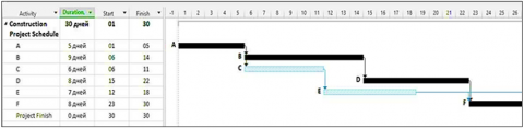
Take, for example, a building project, which comprises six units of work: A, B, C, D, E, and F (see the diagram). Each activity is linked via the "Finish/Start" type of link to connect it to the next one. Figure 1 shows the timeframes and finishes times of activities determined using the Critical Path technique.
The graphic darkens critical tasks A, B, D, and F. As a result, the project's overall duration, denoted by the acronym target, is shaped by the 30-day critical path.
Figure 1. Timetable for the project, including the average duration of each activity
By choosing the most effective amount and quality of groups, the most appropriate mode of transportation technology, the most effective work methods, and other factors, each specific project development can be considered in compliance with the applicable methodology. Typically, method statements are employed to estimate the duration of construction and installation projects. The most effective times are those that cost the least.
Individual project tasks might be expedited at the same time. Project managers can identify potential shortcuts (utilizing stronger machinery or resources with differing qualities, for instance) and the minimum durations that can be achieved for each task even before the project begins. The links must also be optimized so that subsequent operations can get underway as quickly as feasible.
Table 1. Project's start and end dates
|
Actions |
Measurement Time, tmt, Tbsln Times |
Possible Minimum Time, tpmt, Tmin Times |
|
A |
8 |
8 |
|
B |
7 |
6 |
|
C |
8 |
4 |
|
D |
6 |
5 |
|
E |
9 |
8 |
|
F |
5 |
3 |
Almost often, a reduction in work time results in a rise in costs. Let's imagine, however, that the project planning is willing to enhance the budget for the project to ensure the timely completion of the project. Look at the shortest potential activity durations (tpmt) in Table 1 and compare them to the longest possible baseline durations (tmt).
Tbsln: Standard measure (calculated) duration of both the critical route.
Tmin: Minimal potential time for a critical activity.
$K_s=\frac{t m t}{t p m t}$ (4)
Another requirement is that the operations of the project need to be combined in this scenario so that it can be completed more quickly. As an illustration, activity B could be started two days before activity A is finished, and action D could be started one day already when activity B is finished. Both examples refer to the same overall timeline. In this scenario, the time of the important path will be 3 minus 2 plus 8 minus 1 plus 4 plus 8=20 times if the project acceleration is at its maximum.
However, getting approval for the standard date and time of project tasks, as well as their absolute minimum time duration, is required when the standard plan is trained. This is because the minimum possible durations can have a significant impact on the overall success of the project. This provides significant benefits in terms of the Risk Management Process, specifically the shift of construction projects into the "accelerate mode" if critical differences from the baseline approved arise.
The tracking technique doesn't get started until after the Status Of the project dates have been approved and the project has gotten underway. Assume that the Project has been operational for ten days at this point. There was a disparity between the actual time that action A took place and the duration that was determined to be its baseline, which was 10 days. Because the duration of action A must now be extended, the subsequent actions B and D cannot commence until the 11th day instead of the 6th day as originally planned.
After analyzing the data, we are able to arrive at the quality evaluations of the current plan performance status of building projects, which are as follows: "The Delay was Caused" and "The Effect of Delay Is 5 Days." In terms of both quantity and value, the formula can be used to assess the likelihood of accomplishing the strategic objective of completing the project on time (1). As of the tenth day, VT(t=10)=-5 days, which is the number of days that separate the date that the project is finished and the date on which the report is due. the degree of association between the A action period deviation and the B activity date deviation the criticality of the A activity, which accounted for the majority of the project's deviation value, increased the total duration of the project.
Even if the deadline for a project is fulfilled, the approaches that are used today are unable to determine whether or not the goal can be achieved (or impossible). If the project manager recognizes that the delay can be reduced within the remaining time and accepted, there are many options available; however, it is essential to determine which alternative is the most cost-effective in addition to having the most credibility overall.
If all remaining activities are completed within the basic parameters, then our example project will require 25 additional days to be finished. This equates to 9 days plus 8 days plus 8 days plus 8 days. This indicates that the project will not be finished until the 35th day, which is five days later than the goal date alone. On the other hand, it is possible to finish the project in just 19 days if all of the activities are finished in the lowest time possible (as shown in Table 1), which would cut the overall amount of time needed for the project by eight days. Even if it only takes 29 days to finish the project, that will still put it ahead of schedule.
If this is indeed the case, then B and D might have started on day 11. When working on ongoing projects, it is essential to have an accurate estimation of when they will be finished. Let's say that the work at job B is finished on day 19. If we apply the maximum possible acceleration, it is anticipated that the project will be finished in no more than 30 days; this indicates that it will be completed on time.
Following the actual data collection that took place on day 12, the associated tracking revealed that the end date of the B activity would be on day 20. Even if the project is hurried along to the fullest extent of its capabilities, it will not be finished by the end of the thirty-first day.
The preceding illustration serves to show a well-known fact, namely, that the estimated amount of time needed to complete the entire project would increase as the durations of the activities are steadily increased (or start dates are delayed). It has been determined that the slowness that results from watching television cannot be made up for by increasing the speed of other tasks. At this point, the likelihood of a project being successful is extremely remote, if not completely nonexistent.
Because of the way our scales are calibrated, we know that day 11 marks the beginning of the end of our journey.
As was mentioned earlier, the primary objective of managing the time associated with a project is to reduce the likelihood of the project going past the End of the Road. As a consequence of this, the detailed project modification system will be triggered if the current status of the project becomes closer and closer to completion. To clarify, the gap in time between the maximum allowed and the minimum attainable durations of the project serves as a safety buffer of time that should not be used all at once but rather spread out throughout the complete implementation time for the project. The use of this time management tool will allow project managers to steer clear of disastrous outcomes for their projects.
The importance of having a "margin of safety" for project control may be understood from the example given above [25]. The well-being aspect, calculated as a ratio of the maximum weight that a structure can support, must also be considered in structural calculations. Let's introduce a safety factor on time Ks for project management purposes equal to the predicted critical path length divided by the shortest possible critical path duration. The protective immune coefficient rises in value as the likelihood of exceeding a project deadline decreases. Our protective immune coefficient is roughly 30/20=1.5.
Thus, it is vital to propose a methodology that ensures that the critical values will not be approached and that the maintenance schedule will be evenly distributed during the project. At the start of the project, consider the following two Boolean (logic) functions, which can return either a result of one (true) or a result of zero (false).
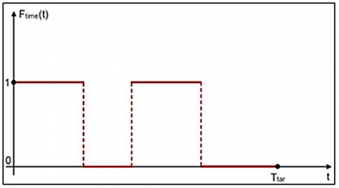
(a) The first function is to ensure that the project is completed on schedule, where Ftime (t)=1, and if VT≥0; so, if VT 0 then Ftime (t)=0, as shown in Figure 2.
Figure 2. Result of the project's finishing time
(b) The second role is the ability to complete the project on time (t).
Ftime(t)=1 when it is possible to complete the project in a timely manner even though the project is behind schedule; otherwise, Ftime(t)=0. A critical component of this function, as depicted in Figure 3, is the requirement that because it equals zero, this will never rebound to one.
Figure 3. Possibility of finishing the project on time
It is obvious that the activity can be finished on schedule as long as the anticipated project length at time t somehow doesn't exceed the permitted one. Thus, the probability that a project would be completed on time can sometimes be zero. The function assessing the completion of the project time is also zero in this situation and cannot be changed back to its initial value of one, which is the opposite of what happens if the function measuring the chance of timely completion of a project is equal to zero.
The Breaking point can be defined as the point at which the ability to complete the project on time no longer exists. If any key activity is delayed by even a fraction of a second, the project's deadline will be jeopardized, regardless of how small the delay is. When the project is nearing its end, the project manager should be informed. The building contractor has no safety margin when the Breaking point is struck at the beginning of a project, and any minor setback will result in a missed deadline for the entire project. The ability to monitor a project's progress and predict when the Snapping point will be achieved is essential for ensuring that, but in the worst situation, the project can be completed as quickly as is practical.
Part of this problem has been answered by one of the articles in this collection, which recommends a construction component of the project management approach targeted at avoiding project disaster and ensuring timely project completion. Schedule Progress Index (SPI) and the Schedule Timeliness Index (STI). When STI and SPI are two different indices that are continuously monitored to gauge the project's progress (SPI). The percentage of time left before the project's officially endorsed end date is the project completion date as of the status date (STI).
$S T I_t=\frac{V T}{T_{\text {target }}-T_{s t d}}$ (5)
where, Tstd=status date.
It is important to pay attention to the project time variation rate as the project nears completion. Due to its relative nature, the Schedule Timeliness Index may track remaining time and hence identify the amount to which the current departure affects project outcomes. Proportional to the remaining time till project completion, SPI is the functionality of determining how much work has been performed to how much work is still to be done. The formula for computing SPI:
$S P I_t=\frac{\frac{N_{\text {complete }}-1}{N_{\text {plan }}}}{\left(T_{\text {target }}-t_{\text {std }}\right)} \times T_{\text {target }}$ (6)
where,
Ncomplete: The extent of work that was finished from now to the status date.
Nplan: The amount of work that needs to be done from now to the status date.
SPI is a supplement, but STI is advised as the main foundation. Establishing the crucial parameters of Indices that can alter the project state is crucial for project time control. It is feasible to locate in one of the regions listed in Table 2 to execute the project on schedule. The remaining plan will be examined, and action will be done to hasten the project's completion date if the project's rating changes from green to yellow. The project is considered a failure and cannot be saved if its status switches from yellow to red.
Table 2. Boundaries of the critical indexes
|
Project Zones |
Index Value |
|
Bright green |
In a scale of zero to L1 |
|
Green |
Over zero |
|
Red |
Just under the level of L2 |
|
Yellow |
Between the ranges L1 to L2 |
The crucial borders of the L1 and L2 Indices are not addressed in our research; nonetheless, it should be noted that the significance values of such Indices depend on the national average of the "margin" size that is stored throughout the schedule calculations.
Let's look at the notions of the duration protective immune coefficient Ks and the indices' value crucial borders and see how they compare with one another. According to the calendar plan safety, the critical route of our project is less stressful in terms of its reserves the larger this safety margin coefficient is.
For example, the margin of safety in our scenario is 1.5, which is equal to fifty percent. The job will not be finished on schedule if the activity durations grow by much more than 1.5 times. It's possible to keep the project on schedule even if the time of the activities increases by a smaller amount. Linear dependence in this context can only ever be an acceptable measure of the true link between these activities because each important action has its own limit of compression.
The case study will move forward at this point. The duration of the project is the most crucial factor to consider; as a result, let's establish various dependencies for some time like the one indicated, which goes from t=0 to t=12.
1. Function that is linear in the time that is left on the project Fr(t).
2. Calculations of a similar nature are carried out on each day t of the project's execution, and thus allow for the non-linear decline function Fdv1(t) to determine the greatest value that is practically attainable for the project date deviation (i.e., Project activities can be accelerated to compensate for any delays that occur daily).
3. When the project's safety factor is set at 1.5, the maximum value of the project dates' deviation that is considered acceptable is defined by the formula Fdv2(t). This is a function that decreases linearly with time. To get the function's output, subtract the outstanding construction schedule from the "allowed" margin's volume. For example, the midpoint value of F(t=30/2=15) is equal to 10 divided by 5, the starting value of F(t0) is equal to 30-30 divided by 1.5 percent, and so on.
4. The data collected during the first nine days of the project have been utilized as an illustration in the preceding case.
5. VT1(t)-The purpose of this study is to investigate the absolute deviation that was calculated at the point in time when the project was being carried out (data as of 10, 11, and 12 days).
6. A function referred to as the project time standard difference, or VT2(t), is estimated using the presumption that the actual time of each active action and the true delay of the time of each critical connection will be extended by a construction safety standardized coefficients of equal to 1.5.
7. Deviation of the project STI1, also known as the Schedule Completion Index, is generated using VT1.
8. The project variation's VT2 value was used to calculate the STI2 plan completion index. Table 3 in the section below contains the results.
Figure 4. The VT1(t), Fdv1(t) activities (t)
The task Final stop, which serves as an example throughout this essay, was carried out on day 12. According to the information presented in Table 3, the line Fdv1(t) depicted in Figure 4 was traversed at this time. According to the data presented in Figure 5, the values returned by the functions VT2(t) and Fdv2(t) were the same at the same time.
Figure 5. VT2(t), Fdv2 are activities (t)
Figure 6. Fdv1 vs. Fdv2
Additionally, it is important to point out that the prevalence of shifting over continuing support does, in fact, work. When various resources are available to accelerate all of these key operations and when distinct consequences (or inconsistencies) of time advance values, Fdv1(t) and Fdv2(t) do not often coincide. This is also the case when separate values are being advanced. Because it is difficult to determine Fdv1(t) using an analytical method, the deviation-derived values VT(t) are typically established by making use of the linear function Fdv2 in the majority of cases (t). In this particular illustration, the difference between Fdv1(t) and Fdv2(t) can be as high as 39 percent.
This discussion focuses on the process by which a project moves from the yellow zone into the red zone shown in Figure 4 and Figure 5 as a result of a STI level of significance (i.e., Arrival at the End of The Road). The quantity of Rank L2 boundaries required can be determined using the link below:
$L_2=1-\frac{1}{K_2}$ (7)
Also, in order to account for the range of the nonlinear function Fdv1, as well as the lineal functional Fdv2(t) departure value, a decreasing coefficient might be brought in (t). On the other hand, the purpose of this essay is not to study how to determine coefficient values.
No matter what happens, L2 can't be higher than the figure that was determined using the formula (2).
The comparison between Fdv1 vs. Fdv2 shown in Figure 6 and this shows that the time difference is near to close.
The suggested value for L1 is fifty percent of L2, which is the point where the light turns from green to yellow.
Table 3. Timelines for the plan
|
t, Period |
Fr(t), Period |
VT1(t), Period |
VT2(t), Period |
Fdv1(t), Period |
Fdv2(t), Period |
STI1(t) |
STI2(t) |
|
0 |
30 |
0 |
0 |
-10 |
-10.0 |
0.000 |
0.000 |
|
1 |
29 |
-0.5 |
-0.5 |
-9.2 |
-9.7 |
-0.017 |
-0.017 |
|
2 |
28 |
-1 |
-1 |
-8.6 |
-9.3 |
-0.036 |
-0.036 |
|
3 |
27 |
-1 |
-1.5 |
-8 |
-9.0 |
-0.037 |
-0.056 |
|
4 |
26 |
-2 |
-2 |
-7 |
-8.7 |
-0.077 |
-0.077 |
|
5 |
25 |
-3 |
-2.5 |
-6 |
-8.3 |
-0.120 |
-0.100 |
|
6 |
24 |
-3 |
-3 |
-5.89 |
-8.0 |
-0.125 |
-0.125 |
|
7 |
23 |
-3 |
-3.5 |
-5.78 |
-7.7 |
-0.130 |
-0.152 |
|
8 |
22 |
-4 |
-4 |
-5.67 |
-7.3 |
-0.182 |
-0.182 |
|
9 |
21 |
-4 |
-4.5 |
-5.56 |
-7.0 |
-0.190 |
-0.214 |
|
10 |
20 |
-5 |
-5 |
-5.45 |
-6.7 |
-0.250 |
-0.250 |
|
11 |
19 |
-5 |
-5.5 |
-5.34 |
-6.3 |
-0.263 |
-0.289 |
|
12 |
18 |
-6 |
-6 |
-5.23 |
-6.0 |
-0.333 |
-0.333 |
The following are some of the conclusions that can be drawn from this study's findings:
1. The primary goal of the project should be to gain control of the project schedule so that it can be completed on time and important milestones can be met. The estimation of the successful delivery date Tforecast in relation to the target date Ttarget, also known as the "Variability Time," is an important part of the project scheduling process. The VT(t) value of a project can become negative as the project progresses, but only if the remaining tasks' completion times are shortened to compensate for the lost time.
2. Prior to accepting the baseline schedule, it is possible to make a preliminary definition of the shortest feasible durations tpmt, I for each project activity by determining the lowest possible costs ci. This can be done prior to the approval of the baseline schedule. Another method for speeding up the operation process is to calculate the maximum potential critical link advance values. Because of this tool, you will always know how much time is left on the project regardless of when you look at it. When the negative value of VT(t) cannot be offset by the maximum potential acceleration of all remaining operations, the End of All Hope is reached. When this happens, the project will unavoidably fail, and the failure will be irreversible.
3. The Schedule Availability Index is a related measure that can be used to estimate the current state of the project based on timeliness requirements. Because of the difficulty in identifying it, the red level of the project's critical value warning signal has been raised. To solve L2, use the construction safety margins factor Ks, which is a relationship between the project's approved duration and its shortest achievable length. Given the erratic nature of the connections between the required minimum duration and the permissible maximum durations of various project activities, the project's state must be evaluated as it progresses from yellow to red. It has been proposed that a value for L1 equal to L1 = 0.5 L2 be used.
[1] Tijanić, K., Car-Pušić, D. (2018). Deadline and budget overruns of construction projects-multiple case-study. Zbornik radova (Građevinski fakultet Sveučilišta u Rijeci), 21(1): 87-101. https://doi.org/10.32762/zr.21.1.5
[2] Vasiljeva, T., Berezkina, E. (2018). Determining project management practices for enterprise resource planning system projects. Journal of Enterprise Resource Planning Studies, 2018: 927123. https://doi.org/10.5171/2018.927123
[3] Zwerenz, D. (2019). Brand management: Organizational changes in project management. Marketing and Management of Innovations, 2: 253-265. http://doi.org/10.21272/mmi.2019.2-22
[4] Alshihri, S., Al-Gahtani, K., Almohsen, A. (2022). Risk factors that lead to time and cost overruns of building projects in Saudi Arabia. Buildings, 12(7): 902. https://doi.org/10.3390/buildings12070902
[5] Krechowicz, M., Piotrowski, J.Z. (2021). Comprehensive risk management in passive buildings projects. Energies, 14(20), 6830. https://doi.org/10.3390/en14206830
[6] Pandey, S., Buyya, R. (2012). A survey of scheduling and management techniques for data-intensive application workflows. In Data Intensive Distributed Computing: Challenges and Solutions for Large-scale Information Management, pp. 156-176. https://doi.org/10.4018/978-1-61520-971-2.ch007
[7] Richardson, G.L., Carstens, D.S. (2021). Project Budgeting. In Guidelines for Achieving Project Management Success, Boca Raton: CRC Press, pp. 63-80.
[8] Kroemer, K.H., Kroemer, H.J., Kroemer-Elbert, K.E. (2020). Body rhythms and work schedules. Engineering Physiology: Bases of Human Factors Engineering/Ergonomics, pp. 263-298. https://doi.org/10.1007/978-3-030-40627-1_10
[9] Lyandau, Y.V. (2022). Project management based on PMBOK 7.0. Imitation Market Modeling in Digital Economy: Game Theoretic Approaches, 368: 283-289.
[10] Cicala, G., Cicala, G. (2020). Introduction to Microsoft project 2019. The Project Managers Guide to Microsoft Project 2019: Covers Standard, Professional, Server, Project Web App, and Office 365 Versions, pp. 31-71. https://doi.org/10.1007/978-1-4842-5635-0_3
[11] Lester, A. (2021). Primavera P2. In Project Management, Planning and Control, Elsevier, pp. 485-503. https://doi.org/10.1016/C2020-0-01597-5
[12] Carstens, D.S., Richardson, G.L., Smith, R.B. (2013). Project Management Tools and Techniques: A Practical Guide. CRC Press.
[13] Lynch, K. (2004). Project management institute (PMI). The Quality Assurance Journal, 8(2): 126-128. https://doi.org/10.1002/qaj.268.
[14] Chiulli, R.M. (2018). Quantitative Analysis. Routledge, London, pp. 159-193. https://doi.org/10.1201/9780203741559
[15] Alvarado, C.M., Silverman, R.P., Wilson, D.S. (2004), Assessing the performance of construction projects: Implementing earned value management at the General Services Administration. Journal of Facilities Management, 3(1): 92-105. https://doi.org/10.1108/14725960510808419
[16] Hua, L.K., Wang, Y., Heijmans, J.G.C. (1989). Program Evaluation and Review Technique (PERT). In: Heijmans, J.G.C. (eds) Popularizing Mathematical Methods in the People’s Republic of China. Mathematical Modeling, vol. 2. Birkhäuser Boston. https://doi.org/10.1007/978-1-4684-6757-4_8
[17] Roos, E., den Hertog, D. (2021). A distributionally robust analysis of the program evaluation and review technique. European Journal of Operational Research, 291(3): 918-928. https://doi.org/10.1016/j.ejor.2020.09.027
[18] Narita, T.T., Alberconi, C.H., de Souza, F.B., Ikeziri, L. (2021). Comparison of PERT/CPM and CCPM methods in project time management. Gepros: Gestão da Produção, Operações e Sistemas, 16(3): 1. https://doi.org/10.15675/gepros.v16i3.2815
[19] Cho, N., El Asmar, M., Gibson Jr, G.E., Aramali, V. (2020,). Earned value management system (EVMS) reliability: A review of existing EVMS literature. In Construction Research Congress 2020: Project Management and Controls, Materials, and Contracts, US, pp. 631-639. https://doi.org/10.1061/9780784482889.066
[20] van Rees, C.B., Hand, B.K., Carter, S.C., et al. (2022). A framework to integrate innovations in invasion science for proactive management. Biological Reviews, 97(4): 1712-1735. https://doi.org/10.1111/brv.12859
[21] de Waal, A. (2013). Implementation of Strategic Performance Management. In Strategic Performance Management, London: Macmillan Education UK, pp. 319-354.
[22] Shaffer, C.A., Kazerouni, A.M. (2021). The impact of programming project milestones on procrastination, project outcomes, and course outcomes: A quasi-experimental study in a third-year data structures course. In Proceedings of the 52nd ACM Technical Symposium on Computer Science Education, US, pp. 907-913. https://doi.org/10.1145/3408877.3432356
[23] Nightingale, A. (2020). Data management plans: Time wasting or time saving? The Biochemist, 42(3): 38-39. https://doi.org/10.1042/BIO20200020
[24] Smith, J.M. (2011). Project Management System. https://doi.org/10.1049/PBPC003E
[25] Wortman, M., Kee, E., Kannan, P. (2020). Safety-Critical Protective Systems and Margins of Safety. arXiv preprint arXiv:2010.09674.