Mimoon Ismael![]() | Shahid Zaman
| Shahid Zaman![]() | Kashif Elahi
| Kashif Elahi![]() | Ali N.A. Koam*
| Ali N.A. Koam*![]() | Ansa Bashir
| Ansa Bashir![]()
© 2024 The authors. This article is published by IIETA and is licensed under the CC BY 4.0 license (http://creativecommons.org/licenses/by/4.0/).
OPEN ACCESS
This article explores a practical applications of chemical graph theory in the field of physical chemistry. Chemical graph theory is a branch of mathematics that uses mathematical techniques to correlate the structural characteristics of molecules. By applying these methods, scientists can better understand how different molecules behave and interact in the world of chemistry. Topological indices, which are two/three-dimensional descriptors of the internal atomic organization of compounds, provide valuable information about the size, shape, branching, presence of heteroatoms, and number of bonds in a given molecular structure. This article highlights the importance of topological indices in understanding the physical properties and behavior of molecules, and how they can be used in various applications such as drug design, material science, and catalysis. In this article, we computed irregularity topological indices for the Oxide network ($O X_n$), Silicate network ($S L_n$), Chain silicate ($C S_n$), and honeycomb network ($H C_n$). The 3D comparison graphs are also investigated. The article concludes with a discussion of the challenges and future directions in the field of chemical graph theory.
nanostructures, oxide network, silicate network, honeycomb network, topological indices, irregularity indices, 3D comparisons
A chemical graph is a representation of a molecule's structure using vertices and edges, where atoms are represented by vertices, and the bonds between atoms are represented by edges. In this graph representation, each atom is a vertex, and the edges connect pairs of atoms that are bonded together. A molecular graph [1, 2] is a straightforward, connected, and undirected finite graph in the context of chemical graph theory and mathematical chemistry [3]. Atoms serve as the nodes' representations, while chemical bonds serve as the edges' descriptions of molecules. Todeschini and Consonni [4] investigated that whether a mathematical formula could be applied to any graph that represents a chemical structure. It is employed for correlation analysis in the fields of toxicology, environmental chemistry, theoretical chemistry, and pharmacology. To determine the degree to which these indicators are connected with one another, however, no systematic investigation has been conducted.
Chemical graph theory, with its focus on topological indices, finds valuable applications in multiple fields. One significant application lies in drug design, where understanding the topology of molecules helps researchers predict their biological activity and interactions, aiding in the development of new pharmaceuticals. In the realm of material science, topological indices provide insights into the properties of materials, helping engineers and scientists tailor materials for specific purposes. Additionally, in the field of catalysis, these indices contribute to unraveling the mechanisms by which catalysts accelerate chemical reactions, leading to advancements in industrial processes and environmental sustainability. In the specific context of the mentioned article, the computation of irregularity topological indices for various network structures, such as Oxide, Silicate, Chain silicate, and honeycomb networks, showcases the versatility of chemical graph theory in studying diverse molecular arrangements and their potential impacts across these applications. In quantum chemistry, understanding the connectivity of atoms in a molecule is crucial for accurate simulations and predictions. Chemical graph theory assists in generating molecular graphs that guide quantum mechanical calculations.
The topological index has gained recognition as a key tool in chemical graph theory for describing the architectures of chemical compounds as time has gone on, according to academics [5]. Ullah et al. [6] demonstrated the relationship between entropy and eccentricity factor made it possible to forecast a number of physicochemical characteristics, including boiling temperature, instance entropy, vaporization enthalpy, and others. Chemical graphs are essentially a branch of mathematical chemistry that employs graph theory to quantitatively represent chemical events [7]. An irregular index is a statistical number associated with a graph that both specify the irregularity of the graph and quantifies how extreme it is [8, 9], according to researches [10, 11]. It is also used for topologically composed non-regular graph numerical analysis. As a result, these indices are highly statistically accurate and useful for QSPR/QSAR research [12-15].
Topological indices play a vital role in the relationships between quantitative structure property and activity, or (QSPR) and (QSAR), respectively. QSAR is a closely related field that focuses on establishing relationships between the chemical structure of molecules and their biological or pharmacological activities. In drug discovery, for instance, QSAR models can help predict how a new compound might interact with a target receptor or enzyme. Chemical graph theory assists in deriving molecular descriptors that capture the relevant structural information, which is then used to build QSAR models. By analyzing the connectivity, branching patterns, and functional groups of molecules, QSAR models can provide insights into the factors that influence a compound's activity, selectivity, toxicity, and other pharmacological properties.
In both QSPR and QSAR, chemical graph theory serves as the foundation for generating meaningful molecular descriptors, which in turn enable the development of predictive models. These models are invaluable tools in drug discovery, materials design, toxicology assessments, and more, as they accelerate research and decision-making processes while reducing costs associated with experimental testing.
The QSAR/QSPR approaches are predicated on the idea that a particular chemical compound's activity such as a medicine binding to DNA or poisonous effect relates to its structure through a specific mathematical formula. A chemical compound's molecular structure will be related to its properties or biological activity. The prediction, interpretation, and evaluation of novel compounds with desired activities or qualities can therefore be done using this connection, lowering and rationalizing the time, effort, and expense of synthesis as well as the cost of developing new products. We recommend references [16-18] for more research on the physico-chemical characteristics. Vallet-Regí et al. [19-24] give some literature review about the degree based topological indices.
The first and most extensively researched topological index in chemical graph theory from a theoretical and practical standpoint is the Wiener index. First introduced as the route index, the Wiener index became named as such in 1947 [25]. To accurately assess the structural characteristics and bioactivity of chemical substances, it is necessary to summarize the structure activity of topological indices. The specifics of a few chemical structure families are addressed in references [26, 27]. As a vertex $Z \in V(G)$, We employ the symbol $\mathrm{Q}(Z)$ for the accumulation of vertices close to $Z$. The degree of a vertex $Z$ is the cardinality of the set $Q(Z)$ and is denoted by $d(Z)$. Let $\varepsilon(\mathrm{z})$ denote the sum of degrees of the vertices adjacent to $Z$. In other words, $\quad \varepsilon(z)=\sum_{\mathrm{uv} \in E(G)} \mathrm{du}$ and $Q(m)=\{v \in$ $V(G) \mid \mathrm{mv} \in E(G)\}$. For the undefined terminologies related to graph theory, one can read references [28-30]. Consider, the following general graph invariant:
$\mathrm{I}(\mathrm{G})=\sum_{\mathrm{v} z \in \mathrm{E}(\mathrm{G})} f(\varepsilon(v), \varepsilon(z))$
Some special cases of the above invariants $I(G)$ have already been appeared in mathematical chemistry. For example, if we take $\mathrm{f}(\varepsilon(\mathrm{v}), \varepsilon(\mathrm{z}))=\varepsilon(\mathrm{v}) \varepsilon(\mathrm{z})$ or $1 / \sqrt{\varepsilon(v) \varepsilon(\mathrm{z})}$.
In this article, we presented the irregularity topological indices for oxide network (OXn), silicate network (SLn), chain silicate (CSn), and honeycomb network (HSn). For other topological indices of OXn, SLn, CSn and HCn are calculated in references [31, 32].
Albertson [7] introduced:
$LA(G)=2\sum\limits_{uv\in E(G)}{\frac{|{{R}_{u}}-{{R}_{v}}|}{|{{R}_{u}}+{{R}_{v}}|}}=\text{-6}\text{.9497n+4}\text{.3598}$
Vukicevic [33] introduced:
$IRL(G)=\sum\limits_{uv\in E(G)}{|\ln {{R}_{u}}-\ln {{R}_{v}}|}$
Vukicevic [33] introduced:
$IRLU(G)=\sum\limits_{uv\in E(G)}{\frac{|{{R}_{u}}-{{R}_{v}}|}{\min ({{R}_{u}},{{R}_{v}})}}$
Abdoo et al. [9] introduced:
$IRRT(G)=\frac{1}{2}\sum\limits_{uv\in E(G)}{|{{R}_{u}}-{{R}_{v}}|}$
Li et al. [34] introduced:
$IRF(G)={{\sum\limits_{uv\in E(G)}{(\mathop{R}_{u}-\mathop{R}_{v})}}^{2}}$
Furthermore, Reti et al. [35] introduced the following indices.
$\begin{align} & IRA(G)={{\sum\limits_{uv\in E(G)}{({{\mathop{R}_{u}}^{-\frac{1}{2}}}-{{\mathop{R}_{v}}^{-\frac{1}{2}}})}}^{2}}, \\ & IRLF(G)=\sum\limits_{uv\in E(G)}{\frac{|{{R}_{u}}-{{R}_{v}}|}{\sqrt{{{R}_{u}}\times {{R}_{v}}}}}, \\ & LA(G)=2\sum\limits_{uv\in E(G)}{\frac{|{{R}_{u}}-{{R}_{v}}|}{|{{R}_{u}}+{{R}_{v}}|}}, \\ & IRDI(G)=\sum\limits_{uv\in E(G)}{\ln (1+|{{R}_{u}}-{{R}_{v}}|}), \\ & IRGA(G)=\sum\limits_{uv\in E(G)}{\ln \frac{|{{R}_{u}}+{{R}_{v}}|}{2\sqrt{{{R}_{u}}\times {{R}_{v}}}}}, \\ & IRB(G)={{\sum\limits_{uv\in E(G)}{({{\mathop{\text{R}}_{u}}^{\frac{1}{2}}}-{{\mathop{R}_{v}}^{\frac{1}{2}}})}}^{2}} \\\end{align}$
For the purpose of planning and forecasting diverse networks, graph theory is a discipline of mathematics. The mathematical tools known as topological invariants are used to examine the connectivity characteristics of a certain network. To explore the characteristics of any chemical network, a wide range of graph in terms of vertex degrees. In chemistry, graph invariants are used as structural descriptors, are with the key reasons to research them [36, 37].
2.1 Oxide network
In the investigation of silicate networks, the oxide network is crucial. After removing the silicon vertices from a silicate network, an oxide network can be developed $O X_n$ (See Figure 1). The n-dimensional oxide network is denoted as $O X_n$. In the oxide network, the number of vertices is 9 $n^2+3 n$ and number of edges are 18 $n^2$ correspondingly.
According to the degree summing of the peers of the end vertices, the edge set in $O X_n$ may be split up into six sets, as shown in Table 1.
Figure 1. An oxide network $\mathrm{O}{X}_2$
2.2 Honeycomb network
A hexagon forms the honeycomb network. By attaching six hexagons to the boundary edges of an experimentally synthesized network, the honeycomb network is constructed (see Figure 2). It is accessible through HCn-1 by encircling the edge of the field with a layer of hexagons HCn-1.
We use n hexagons to illustrate an n-dimensional honeycomb structure HCn. By placing a layer of hexagons around it, the honeycomb network is preserved HCn-1. The order and size of HCn is 6n2 and 9n2-3n, respectively.
Figure 2. A honeycomb network HCn
2.3 Silicate network
The bulk of the minerals that build up the rocks that form the crust of the Earth is silicates. These include a wide range of clay minerals as well as minerals including quartz, feldspar, mica, amphibole, pyroxene, and olivine. A silicate sheet is a ring of tetrahedrons connected to other rings in a two-dimensional plane by nodes that share oxygen to form a structure that resembles a sheet. On a graphic, we designate the central atom as silicon, the corner atoms as oxygen, and the edges as the connections between them. A silicate array with n hexagons between the center and edge of the silicate sheet is represented by the symbol $S L_n$. In Figure 3, we presented a three-dimensional $S L_n$ with order and size is $15 n^2+3 n$ and $36 n^2$, respectively.
Figure 3. A Silicate network $\mathrm{S} L_n$
2.4 Chain silicate network
Tetrahedral n-dimensional linear configuration yields chain silicate, which has the essential specifications. A network of n-dimensional chain silicate, designated by the symbol $C S_n$ , is created by stacking n tetrahedrons in a linear configuration with order and size of the parameters is 3n+1 and 6n, respectively. It has shown in Figure 4.
Figure 4. A chain silicate network CSn
Table 1. Edge partition of OX2
|
(ε(v), ε(z)) |
Cardinality |
|
(8, 12) |
12 |
|
(12, 14) |
12 |
|
(16, 16) |
18n2-36n+18 |
|
(8, 14) |
12(n-1) |
|
(14, 16) |
12(n-1) |
|
(14, 14) |
6(2n-3) |
Table 2. Edge partition of H$C_n$
|
(ε(v), ε(z)) |
Cardinality |
|
(5, 5) |
6 |
|
(5, 7) |
12(n-1) |
|
(7, 9) |
6(n-1) |
|
(9, 9) |
9n2-21n+12 |
Table 3. Edge partition of S$L_n$
|
(ε(v), ε(z)) |
Cardinality |
|
(15, 15) |
6n |
|
(18, 27) |
12(n-1) |
|
(27, 30) |
12(n-1) |
|
(18, 30) |
18n2-30n+12 |
|
(15, 27) |
24(n-1) |
|
(24, 27) |
12 |
|
(15, 24) |
24 |
|
(27, 27) |
6(2n-3) |
|
(30, 30) |
18n2-36n+18 |
Table 4. Edge partition of C$S_n$
|
(ε(v), ε(z)) |
Cardinality |
|
(12, 12) |
6 |
|
(12, 21) |
6 |
|
(15, 15) |
n-2 |
|
(15, 21) |
4 |
|
(15, 24) |
4n-12 |
|
(21, 24) |
2 |
|
(24, 24) |
n-4 |
Theorem 3.1: Let O$X_2$ be an oxide network as depicted in Figure 1, then based on Table 1 we have the following results.
a) $A L\left(O X_2\right)=96 n-24$
b) $\operatorname{IRL}\left(O X_2\right)=8.3106 \mathrm{n}-1.5948$
c) $\operatorname{IRLU}\left(O X_2\right)=10.714 \mathrm{n}-2.7142$,
d) $\operatorname{IRRT}\left(O X_2\right)=48 \mathrm{n}-12$,
e) $\operatorname{IRF}\left(O X_2\right)=480 \mathrm{n}-360$,
f) $\operatorname{IRA}\left(O X_2\right)=0.0918 \mathrm{n}-0.003591$
g) $\operatorname{IRDIF}\left(O X_2\right)=17.3472 \mathrm{n}-3.6332$
h) $\operatorname{IRLF}\left(O X_2\right)=8.4069 \mathrm{n}-1.6562$
i) $L A\left(O X_2\right)=8.144 \mathrm{n}-1.484$
j) $\operatorname{IRDI}\left(O X_2\right)=36.53332 \mathrm{n}-4.038$
k) $\operatorname{IRGA}\left(O X_2\right)=0.4884 \mathrm{n}-0.20784$
l) $\operatorname{IRB}\left(O X_2\right)=10.80768 \mathrm{n}-5.0353$
Proof: Based on Table 1 and from definition of AL(G) we have:
(1)
$\begin{align} & AL(O{{X}_{2}})=\sum\limits_{uv\in E(O{{X}_{2}})}{|{{R}_{u}}-{{R}_{v}}|} \\ & =\text{(}{{\text{p}}_{\text{(8,12)}}}\text{) }\!\!|\!\!\text{ 8-12 }\!\!|\!\!\text{ }+\text{(}{{\text{p}}_{\text{(12,14)}}}\text{) }\!\!|\!\!\text{ 12-14 }\!\!|\!\!\text{ }+\text{(}{{\text{p}}_{\text{(16,16)}}}\text{) }\!\!|\!\!\text{ 16-16 }\!\!|\!\!\text{ } \\ & +\text{(}{{\text{p}}_{\text{(8,14)}}}\text{) }\!\!|\!\!\text{ 8-14 }\!\!|\!\!\text{ }+\text{(}{{\text{p}}_{\text{(14,16)}}}\text{) }\!\!|\!\!\text{ 14-16 }\!\!|\!\!\text{ }+\text{(}{{\text{p}}_{\text{(14,14)}}}\text{) }\!\!|\!\!\text{ 14-14 }\!\!|\!\!\text{ } \\ & \text{= }\!\!|\!\!\text{ 8-12 }\!\!|\!\!\text{ (12)+ }\!\!|\!\!\text{ 12-14 }\!\!|\!\!\text{ (12)+ }\!\!|\!\!\text{ 16-16 }\!\!|\!\!\text{ (18}{{\text{n}}^{\text{2}}}\text{-36n+18)} \\ & \text{+ }\!\!|\!\!\text{ 8-14 }\!\!|\!\!\text{ (12(n-1))} \\ & \text{ + }\!\!|\!\!\text{ 14-16 }\!\!|\!\!\text{ (12(n-1))+ }\!\!|\!\!\text{ 14-14 }\!\!|\!\!\text{ (6(2n-3))} \\ & \text{ =96n-24} \\\end{align}$
(2)
$\begin{align} & IRL(O{{X}_{2}})=\sum\limits_{uv\in E(O{{X}_{2}})}{|\ln {{R}_{u}}-\ln {{R}_{v}}|} \\ & =({{p}_{(8,12)}})|\ln 8-\ln 12|+({{p}_{(12,14)}})|\ln 12-\ln 14| \\ & +({{p}_{(16,16)}})|\text{ ln16-ln16 }\!\!|\!\!\text{ }+\text{(}{{\text{p}}_{\text{(8,14)}}}\text{) }\!\!|\!\!\text{ ln8-ln14 }\!\!|\!\!\text{ } \\ & +\text{(}{{\text{p}}_{\text{(14,16)}}}\text{) }\!\!|\!\!\text{ ln14-ln16 }\!\!|\!\!\text{ }+\text{(}{{\text{p}}_{\text{(14,14)}}}\text{) }\!\!|\!\!\text{ ln14-ln14 }\!\!|\!\!\text{ } \\ & =\text{12(2}\text{.0794-2}\text{.4849) +12(2}\text{.4849-2}\text{.63905)} \\ & \text{+ (18}{{\text{n}}^{\text{2}}}\text{-36n+18)(2}\text{.772-2}\text{.772)} \\ & \text{+12(n-1)(2}\text{.0794-2}\text{.639)+12(n-1) (2}\text{.63905-2}\text{.772)} \\ & \text{+6(2n-3)(2}\text{.63905-2}\text{.63905)} \\ & =\text{8}\text{.3106n-1}\text{.5948} \\\end{align}$
(3)
$\begin{align} & IRLU(O{{X}_{2}})=\sum\limits_{uv\in E(O{{X}_{2}})}{\frac{|{{R}_{u}}-{{R}_{v}}|}{\min ({{R}_{u}},{{R}_{v}})}} \\ & =\text{ (12)}\frac{\text{ }\!\!|\!\!\text{ 8-12 }\!\!|\!\!\text{ }}{\text{min(8,12)}}+\text{(12)}\frac{\text{ }\!\!|\!\!\text{ 12-14 }\!\!|\!\!\text{ }}{\min (12,14)} \\ & +(18{{n}^{2}}-36n+18)\frac{|16-16|}{\min (16,16)} \\ & +12(n-1)\frac{|8-14|}{\min (8,14)}+12(n-1)\frac{|14-16|}{\min (14,16)} \\ & +6(2n-3)\frac{|14-14|}{\min (14,14)} \\ & =10.714n-2.7142 \\\end{align}$
(4)
$\operatorname{IRRT}\left(O X_2\right)=\frac{1}{2} \sum_{u v \in E\left(O X_2\right)}\left|R_u-R_v\right|$
$=\frac{1}{2}\left[\left(\mathrm{p}_{(8,12)}\right)|8-12|+\left(\mathrm{p}_{(12,14)}\right)|12-14|+\left(\mathrm{p}_{(16,16)}\right)|16-16|\right.$
$\left.+\left(\mathrm{p}_{(8,14)}\right)|8-14|+\left(\mathrm{p}_{(14,16)}\right)|(14-16)|+\left(\mathrm{p}_{(14,14)}\right)|14-14|\right]$
$\begin{aligned} & =\frac{1}{2}\left[12(4)+12(2)+\left(18 n^2-36 n+18\right)(0)+12(n-1)(4)\right. \\ & +12(n-1)(2)+6(2 n-3)(0)] \\ & =48 n-12\end{aligned}$
(5)
$\begin{aligned} & \operatorname{IRF}\left(\mathrm{OX}_2\right)=\sum_{u v \in E\left(O X_2\right)}\left|R_u-R_v\right|^2 \\ & =12|8-12|^2+12|12-14|^2+\left(18 \mathrm{n}^2-36 \mathrm{n}+18\right)|16-16|^2 \\ & +12(\mathrm{n}-1)|8-14|^2 \\ & +12(\mathrm{n}-1)|14-16|^2+6(2 \mathrm{n}-3)|14-14|^2 \\ & =480 n-360\end{aligned}$
(6)
$\begin{align} & IRA(O{{X}_{2}})=\sum\limits_{uv\in E(O{{X}_{2}})}{|{{\mathop{R_u}}^{-\frac{1}{2}}}-{{\mathop{R_v}}^{-\frac{1}{2}}}}{{|}^{2}} \\ & =\text{ (12)(}{{\text{8}}^{\frac{\text{-1}}{\text{2}}}}\text{-1}{{\text{2}}^{\frac{\text{-1}}{\text{2}}}}{{\text{)}}^{\text{2}}}\text{+12(1}{{\text{2}}^{\frac{\text{-1}}{\text{2}}}}-{{14}^{\frac{-1}{2}}}{{)}^{2}} \\ & +(18{{n}^{2}}-36n+18){{({{16}^{\frac{-1}{2}}}-{{16}^{\frac{-1}{2}}})}^{2}} \\ & +12(n-1){{({{8}^{\frac{-1}{2}}}-{{14}^{\frac{-1}{2}}})}^{2}}+12(n-1){{({{14}^{\frac{-1}{2}}}-{{16}^{\frac{-1}{2}}})}^{2}} \\ & +6(2n-3){{({{14}^{\frac{-1}{2}}}-{{14}^{\frac{-1}{2}}})}^{2}} \\ & =\text{0}\text{.0918n-0}\text{.003591 } \\\end{align}$
(7)
$\begin{align} & IRDIF(O{{X}_{2}})=\sum\limits_{uv\in E(O{{X}_{2}})}{|\frac{{{R}_{u}}}{{{R}_{v}}}-\frac{{{R}_{v}}}{{{R}_{u}}}|} \\ & =(12)|\frac{8}{12}-\frac{12}{8}|+(12)|\frac{12}{14}-\frac{14}{12}| \\ & +(18{{n}^{2}}-36n+18)|\frac{16}{16}-\frac{16}{16}| \\ & +12(n-1)|\frac{8}{14}-\frac{14}{8}|+12(n-1)|\frac{14}{16}-\frac{16}{14}| \\ & +6(2n-3)|\frac{14}{14}-\frac{14}{14}| \\ & =\text{17}\text{.3472n-3}\text{.6332} \\\end{align}$
(8)
$\begin{aligned} & \operatorname{IRLF}\left(O X_2\right)=\sum_{u v \in E\left(O X_2\right)} \frac{\left|R_u-R_v\right|}{\sqrt{R_u \times R_v}} \\ & =(12) \frac{|8-12|}{\sqrt{(8 \times 12)}}+(12) \frac{|12-14|}{\sqrt{(12 \times 14)}} \\ & +\left(18 n^2-36 n+18\right) \frac{|16-16|}{\sqrt{(16 \times 16)}}+12(n-1) \frac{|8-14|}{\sqrt{(8 \times 14)}} \\ & +12(n-1) \frac{|14-16|}{\sqrt{(14 \times 16)}}+6(2 n-3) \frac{|14-14|}{\sqrt{(14 \times 14)}} \\ & =8.4069 n-1.6562\end{aligned}$
(9)
$\begin{aligned} & L A\left(O X_2\right)=2 \sum_{u v \in E\left(O X_2\right)} \frac{\left|R_u-R_v\right|}{R_u+R_v \mid} \\ & =2\left[(12) \frac{|8-12|}{(8+12)}+(12) \frac{|12-14|}{(12+14)}\right. \\ & +\left(18 n^2-36 n+18\right) \frac{|16-16|}{(16+16)}+12(n-1) \frac{|8-14|}{(8+14)} \\ & \left.+12(n-1) \frac{|14-16|}{(14+16)}+6(2 n-3) \frac{|14-14|}{(14+14)}\right] \\ & =8.144 n-1.484\end{aligned}$
(10)
$\begin{align} & IRDI(O{{X}_{2}})=\sum\limits_{uv\in E(O{{X}_{2}})}{\ln (1+|{{R}_{u}}-{{R}_{v}}|}) \\ & =\text{ }\!\!|\!\!\text{ }{{\text{p}}_{\text{(8,12)}}}\text{ }\!\!|\!\!\text{ ln(1}+\text{(8-12))}+\text{ }\!\!|\!\!\text{ }{{\text{p}}_{\text{(12,14)}}}\text{ }\!\!|\!\!\text{ ln(1}+\text{(12-14))} \\ & +\text{ }\!\!|\!\!\text{ }{{\text{p}}_{\text{(16,16)}}}\text{ }\!\!|\!\!\text{ ln(1}+\text{(16-16))}+\text{ }\!\!|\!\!\text{ }{{\text{p}}_{\text{(8,14)}}}\text{ }\!\!|\!\!\text{ ln(1}+\text{(8-14))} \\ & +\text{ }\!\!|\!\!\text{ }{{\text{p}}_{\text{(14,16)}}}\text{ }\!\!|\!\!\text{ ln(1}+\text{(14-16))}+\text{ }\!\!|\!\!\text{ }{{\text{p}}_{\text{(14,14)}}}\text{ }\!\!|\!\!\text{ ln(1}+\text{(14-14))} \\ & =\text{ (12)ln(1+(8-12))+(12) ln(1+(12-14))} \\ & \text{+(18}{{\text{n}}^{\text{2}}}\text{-36n+18) ln(1+(16-16))} \\ & \text{+12(n-1)ln(1+(8-14))+12(n-1) ln(1+(14-16))} \\ & \text{+6(2n-3)ln(1+(14-14))} \\ & =\text{36}\text{.53332n-4}\text{.038} \\\end{align}$
(11)
$\begin{align} & IRGA(O{{X}_{2}})=\sum\limits_{uv\in E(O{{X}_{2}})}{\ln \frac{|{{R}_{u}}+{{R}_{v}}|}{2\sqrt{{{R}_{u}}\times {{R}_{v}}}}} \\ & =\text{ (12)ln}\frac{\text{ }\!\!|\!\!\text{ 8}+\text{12 }\!\!|\!\!\text{ }}{2\sqrt{(8\times 12)}}+\text{(12)ln}\frac{\text{ }\!\!|\!\!\text{ 12}+\text{14 }\!\!|\!\!\text{ }}{2\sqrt{(12\times 14)}} \\ & +(18{{n}^{2}}-36n+18)\ln \frac{|16+16|}{2\sqrt{(16\times 16)}} \\ & +12(n-1)\ln \frac{|8+14|}{2\sqrt{(8\times 14)}}+12(n-1)\ln \frac{|14+16|}{2\sqrt{(14\times 16)}} \\ & +6(2n-3)\ln \frac{|14+14|}{2\sqrt{(14\times 14)}} \\ & =\text{0}\text{.4884n-0}\text{.20784} \\\end{align}$
(12)
$\begin{aligned} & \operatorname{IRB}\left(O X_2\right)=\sum_{u v \in E\left(O X_2\right)}\left|R_u^{\frac{1}{2}}-R_v^{\frac{1}{2}}\right|^2 \\ & =(12)\left|8^{\frac{1}{2}}-12^{\frac{1}{2}}\right|^2+12\left|12^{\frac{1}{2}}-14^{\frac{1}{2}}\right|^2 \\ & +\left(18 n^2-36 n+18\right)\left|16^{\frac{1}{2}}-16^{\frac{1}{2}}\right|^2 \\ & +12(n-1)\left|8^{\frac{1}{2}}-14^{\frac{1}{2}}\right|^2+12(n-1)\left|14^{\frac{1}{2}}-16^{\frac{1}{2}}\right|^2 \\ & +6(2 n-3)\left|14^{\frac{1}{2}}-14^{\frac{1}{2}}\right|^2 \\ & =10.80768 \mathrm{n}-5.0353\end{aligned}$
Theorem 3.2: Let HCn be a honeycomb network as depicted in Figure 2, then based on Table 2, we have the following results.
a) $A L\left(H C_n\right)=36 n-36$
b) $\operatorname{IRL}\left(H C_n\right)=5.538 \mathrm{n}-5.538$
c) $\operatorname{IRLU}\left(H C_n\right)=6.514 \mathrm{n}-6.514$
d) $\operatorname{IRRT}\left(H C_n\right)=18 \mathrm{n}-18$
e) $\operatorname{IRF}\left(H C_n\right)=72 \mathrm{n}-72$
f) $\operatorname{IRA}\left(H C_n\right)=0.06960 \mathrm{n}-0.06960$
g) $\operatorname{IRDIF}\left(H C_n\right)=11.2758 \mathrm{n}-11.2758$
h) $\operatorname{IRLF}\left(H C_n\right)=5.5678 \mathrm{n}-5.5678$
i) $L A\left(H C_n\right)=5.5 \mathrm{n}-5.5$
j) $\operatorname{IRDI}\left(H C_n\right)=19.774 \mathrm{n}-19.774$
k) $\operatorname{IRGA}\left(H C_n\right)=47.4135 \mathrm{n}-47.4135$
l) $\operatorname{IRB}\left(H C_n\right)=2.76654 \mathrm{n}-2.76654$
Proof: Based on Table 2 and from definition of AL(G) we have
(1)
$\begin{align} & AL(H{{C}_{n}})=\sum\limits_{uv\in E(H{{C}_{n}})}{|{{R}_{u}}-{{R}_{v}}|} \\ & =|{{p}_{(5,5)}}|(5-5)+|{{p}_{(5,7)}}|(5-7)+|{{p}_{(7,9)}}|(7-9) \\ & +|{{p}_{(9,9)}}|(9-9) \\ & =\text{6(0)+12(n-1)(2)+6(n-1)(2)+ (9}{{\text{n}}^{\text{2}}}\text{-21n+12)(0)} \\ & \text{=36n-36} \\\end{align}$
(2)
$\begin{align} & IRL(H{{C}_{n}})=\sum\limits_{uv\in E(H{{C}_{n}})}{|\ln {{R}_{u}}-\ln {{R}_{v}}|} \\ & =({{p}_{(5,5)}})|\ln 5-\ln 5|+({{p}_{(5,7)}})|\ln 5-\ln 7| \\ & +({{p}_{(7,9)}})|\ln 7-\ln 9|+({{p}_{(9,9)}})|\ln 9-\ln 9| \\ & =\text{(6)(0)+12(n-1)(0}\text{.336)+6(n-1)(0}\text{.251)+0} \\ & \text{=5}\text{.538n-5}\text{.538} \\\end{align}$
(3)
$\begin{align} & IRLU(H{{C}_{n}})=\sum\limits_{uv\in E(H{{C}_{n}})}{\frac{|{{R}_{u}}-{{R}_{v}}|}{\min ({{R}_{u}},{{R}_{v}})}} \\ & =(6)\frac{|5-5|}{\min (5,5)}+12(n-1)\frac{|5-7|}{\min (5,7)} \\ & +6(n-1)\frac{|7-9|}{\min (7,9)}+(9{{n}^{2}}-21n+12)\frac{|9-9|}{\min (9,9)} \\ & =\text{6}\text{.514n-6}\text{.514} \\\end{align}$
(4)
$\begin{align} & IRRT(H{{C}_{n}})=\frac{1}{2}\sum\limits_{uv\in E(H{{C}_{n}})}{|{{R}_{u}}-{{R}_{v}}|} \\ & =\frac{1}{2}[|{{p}_{(5,5)}}|(5-5)+|{{p}_{(5,7)}}|(5-7) \\ & +|{{p}_{(7,9)}}|(7-9)+|{{p}_{(9,9)}}|(9-9)] \\ & =\frac{1}{2}\text{ }\!\![\!\!\text{ 6(0)+12(n-1)(2)+6(n-1)(2)+ (9}{{\text{n}}^{\text{2}}}\text{-21n+12)(0) }\!\!]\!\!\text{ } \\ & =\text{18n-18} \\\end{align}$
(5)
$\begin{align} & IRF(H{{C}_{n}})={{\sum\limits_{uv\in E(H{{C}_{n}})}{(\mathop{R_u}-\mathop{R_v})}}^{2}} \\ & =|{{p}_{(5,5)}}|{{(5-5)}^{2}}+|{{p}_{(5,7)}}|{{(5-7)}^{2}}+|{{p}_{(7,9)}}|{{(7-9)}^{2}} \\ & +|{{p}_{(9,9)}}|{{(9-9)}^{2}} \\ & =\text{6(0)+12(n-1)(-4)+6(n-1)(-4)+ (9}{{\text{n}}^{\text{2}}}\text{-21n+12)(0)} \\ & \text{=72n-72} \\\end{align}$
(6)
$\begin{align} & IRA(H{{C}_{n}})={{\sum\limits_{uv\in E(H{{C}_{n}})}{({{\mathop{R_u}}^{-\frac{1}{2}}}-{{\mathop{R_v}}^{-\frac{1}{2}}})}}^{2}} \\ & =|{{p}_{(5,5)}}|{{({{5}^{\frac{-1}{2}}}-{{5}^{\frac{-1}{2}}})}^{2}}+|{{p}_{(5,7)}}|{{({{5}^{\frac{-1}{2}}}-{{7}^{\frac{-1}{2}}})}^{2}} \\ & +|{{p}_{(7,9)}}|{{({{7}^{\frac{-1}{2}}}-{{9}^{\frac{-1}{2}}})}^{2}}+|{{p}_{(9,9)}}|{{({{9}^{\frac{-1}{2}}}-{{9}^{\frac{-1}{2}}})}^{2}} \\ & \text{ }=\text{6(0)+12(n-1)(0}\text{.4472-0}\text{.37796}{{\text{)}}^{\text{2}}} \\ & \text{+6(n-1)(0}\text{.37796-0}\text{.333}{{\text{)}}^{\text{2}}}\text{+0} \\ & \text{= 0}\text{.06960n-0}\text{.06960} \\\end{align}$
(7)
$\begin{align} & IRDIF(H{{C}_{n}})=\sum\limits_{uv\in E(H{{C}_{n}})}{|\frac{{{R}_{u}}}{{{R}_{v}}}-\frac{{{R}_{v}}}{{{R}_{u}}}|} \\ & =(6)|\frac{5}{5}-\frac{5}{5}|+12(n-1)|\frac{5}{7}-\frac{7}{5}| \\ & +6(n-1)|\frac{7}{9}-\frac{9}{7}|+(9{{n}^{2}}-21n+12)|\frac{9}{9}-\frac{9}{9}| \\ & \text{=11}\text{.2758n-11}\text{.2758} \\\end{align}$
(8)
$\begin{align} & IRLF(H{{C}_{n}})=\sum\limits_{uv\in E(H{{C}_{n}})}{\frac{|{{R}_{u}}-{{R}_{v}}|}{\sqrt{{{R}_{u}}\times {{R}_{v}}}}} \\ & =(6)\frac{|5-5|}{\sqrt{(5+5)}}+12(n-1)\frac{|5-7|}{\sqrt{(5+7)}} \\ & +6(n-1)\frac{|7-9|}{\sqrt{(7+9)}}+(9{{n}^{2}}-21n+12)\frac{|9-9|}{\sqrt{(9+9)}} \\ & =\text{5}\text{.5678n-5}\text{.5678} \\\end{align}$
(9)
$\begin{align} & LA(H{{C}_{n}})=2\sum\limits_{uv\in E(H{{C}_{n}})}{\frac{|{{R}_{u}}-{{R}_{v}}|}{|{{R}_{u}}+{{R}_{v}}|}} \\ & =2[(6)\frac{|5-5|}{(5+5)}+12(n-1)\frac{|5-7|}{(5+7)} \\ & +6(n-1)\frac{|7-9|}{(7+9)}+(9{{n}^{2}}-21n+12)\frac{|9-9|}{(9+9)}] \\ & =5.5n-5.5 \\\end{align}$
(10)
$\begin{align} & IRDI(H{{C}_{n}})=\sum\limits_{uv\in E(H{{C}_{n}})}{\ln (1+|{{R}_{u}}-{{R}_{v}}|}) \\ & =|{{p}_{(5,5)}}|\ln (1+(5-5)) \\ & +|{{p}_{(5,7)}}|\ln (1+(5-7))+|{{p}_{(7,9)}}|\ln (1+(7-9)) \\ & +|{{p}_{(9,9)}}|\ln (1+(9-9)) \\ & =\text{(6)ln(1+ }\!\!|\!\!\text{ 5-5 }\!\!|\!\!\text{ )+12(n-1) ln(1+ }\!\!|\!\!\text{ 5-7 }\!\!|\!\!\text{ )+6(n-1)ln(1+ }\!\!|\!\!\text{ 7-9 }\!\!|\!\!\text{ )} \\ & \text{+(9}{{\text{n}}^{\text{2}}}\text{-21n+12)ln(1+ }\!\!|\!\!\text{ 9-9 }\!\!|\!\!\text{ )} \\ & =\text{19}\text{.774n-19}\text{.774} \\\end{align}$
(11)
$\begin{align} & IRGA(H{{C}_{n}})=\sum\limits_{uv\in E(H{{C}_{n}})}{\ln \frac{|{{R}_{u}}+{{R}_{v}}|}{2\sqrt{{{R}_{u}}\times {{R}_{v}}}}} \\ & =(6)\ln \frac{(5+5)}{2\sqrt{5\times 5}}+12(n-1)\ln \frac{(5+7)}{2\sqrt{5\times 7}} \\ & +6(n-1)\ln \frac{(7+9)}{2\sqrt{7\times 9}}+(9{{n}^{2}}-21n+12)\ln \frac{(9+9)}{2\sqrt{9\times 9}} \\ & =\text{6(0)+12(n-1)(0}\text{.01408)+6(n-1)(7}\text{.8741)} \\ & \text{+ (9}{{\text{n}}^{\text{2}}}\text{-21n+12)(0)=47}\text{.4135n-47}\text{.4135} \\\end{align}$
(12)
$\begin{align} & IRB(H{{C}_{n}})={{\sum\limits_{uv\in E(H{{C}_{n}})}{|{{\mathop{R_u}}^{\frac{1}{2}}}-{{\mathop{R_v}}^{\frac{1}{2}}}|}}^{2}} \\ & =({{p}_{(5,5)}})|{{5}^{\frac{1}{2}}}-{{5}^{\frac{1}{2}}}{{|}^{2}}+({{p}_{(5,7)}})|{{5}^{\frac{1}{2}}}-{{7}^{\frac{1}{2}}}{{|}^{2}} \\ & +({{p}_{(7,9)}})|{{7}^{\frac{1}{2}}}-{{9}^{\frac{1}{2}}}{{|}^{2}}+({{p}_{(9,9)}})|{{9}^{\frac{1}{2}}}-{{9}^{\frac{1}{2}}}{{|}^{2}} \\ & =(6){{({{5}^{\frac{1}{2}}}-{{5}^{\frac{1}{2}}})}^{2}}+12(n-1){{({{5}^{\frac{1}{2}}}-{{7}^{\frac{1}{2}}})}^{2}} \\ & +6(n-1){{({{7}^{\frac{1}{2}}}-{{9}^{\frac{1}{2}}})}^{2}}+(9{{n}^{2}}-21n+12){{({{9}^{\frac{1}{2}}}-{{9}^{\frac{1}{2}}})}^{2}} \\ & \text{=2}\text{.76654n-2}\text{.76654} \\\end{align}$
Theorem 3.3: Let SLn be silicate network as depicted in Figure 3, then based on Table 3 we have the following results.
a) $A L\left(S L_n\right)=216 n^2+72 n-36$
b) $\operatorname{IRL}\left(S L_n\right)=9.1944 \mathrm{n}^2+4.9118 \mathrm{n}-14.1062$
c) $R L U\left(S L_n\right)=11.88 \mathrm{n}^2+6.73 \mathrm{n}-2.71$
d) $\operatorname{IRRT}\left(S L_n\right)=108 n^2+36 n-28$
e) $\operatorname{IRF}\left(S L_n\right)=2592 \mathrm{n}^2+216 \mathrm{n}-756$
f) $\operatorname{IRA}\left(S L_n\right)=0.05094 \mathrm{n}^2+0.03858-0.02216$
g) $\operatorname{IRDIF}\left(S L_n\right)=19.188 \mathrm{n}^2+10.414 \mathrm{n}-3.369$
h) $\operatorname{IRLF}\left(S L_n\right)=9.2934 \mathrm{n}^2+4.9857 \mathrm{n}-1.4808$
i) $L A\left(S L_n\right)=9 \mathrm{n}^2+4.777 \mathrm{n}-1.29$
j) $\operatorname{IRDI}\left(S L_n\right)=46.152 n^2+28.896 n-3.1505$
k) $\operatorname{IRGA}\left(S L_n\right)=0.5796 \mathrm{n}^2+0.3164 \mathrm{n}-0.21861$
l) $\operatorname{IRB}\left(S L_n\right)=27.432 \mathrm{n}^2+8.154 \mathrm{n}-9.3264$
Proof: Based on Table 3 and from definition of AL(G) we have
(1)
$\begin{align} & AL(S{{L}_{n}})=\sum\limits_{uv\in E(S{{L}_{n}})}{|{{R}_{u}}-{{R}_{v}}|} \\ & =\text{6n }\!\!|\!\!\text{ 15-15 }\!\!|\!\!\text{ +12(n-1) }\!\!|\!\!\text{ 18-27 }\!\!|\!\!\text{ } \\ & \text{+12(n-1) }\!\!|\!\!\text{ 27-30 }\!\!|\!\!\text{ +(18 }{{\text{n}}^{\text{2}}}\text{-30n+12) }\!\!|\!\!\text{ 18-30 }\!\!|\!\!\text{ } \\ & \text{+24(n-1) }\!\!|\!\!\text{ 15- 27 }\!\!|\!\!\text{ +12 }\!\!|\!\!\text{ 24-27 }\!\!|\!\!\text{ } \\ & \text{+24 }\!\!|\!\!\text{ 15-24 }\!\!|\!\!\text{ +6(2n-3) }\!\!|\!\!\text{ 27-27 }\!\!|\!\!\text{ + (18}{{\text{n}}^{\text{2}}}\text{-36n+18) }\!\!|\!\!\text{ 30-30 }\!\!|\!\!\text{ } \\ & \text{=216}{{\text{n}}^{\text{2}}}+\text{72n-36} \\\end{align}$
(2)
$\begin{align} & IRL(S{{L}_{n}})=\sum\limits_{uv\in E(S{{L}_{n}})}{|\ln {{R}_{u}}-\ln {{R}_{v}}|} \\ & =\text{6n }\!\!|\!\!\text{ ln15-ln15 }\!\!|\!\!\text{ +12(n-1) }\!\!|\!\!\text{ ln18-ln27 }\!\!|\!\!\text{ } \\ & \text{+12(n-1) }\!\!|\!\!\text{ ln27-ln30 }\!\!|\!\!\text{ +(18 }{{\text{n}}^{\text{2}}}\text{-30n+12) }\!\!|\!\!\text{ ln18-ln30 }\!\!|\!\!\text{ } \\ & \text{+24(n-1) }\!\!|\!\!\text{ ln15-ln 27 }\!\!|\!\!\text{ +12 }\!\!|\!\!\text{ ln24-ln27 }\!\!|\!\!\text{ } \\ & \text{+24 }\!\!|\!\!\text{ ln15-ln24 }\!\!|\!\!\text{ +6(2n-3) }\!\!|\!\!\text{ ln27-ln27 }\!\!|\!\!\text{ } \\ & \text{+ (18}{{\text{n}}^{\text{2}}}\text{-36n+18) }\!\!|\!\!\text{ ln30-ln30 }\!\!|\!\!\text{ } \\ & \text{=9}\text{.1944 }{{\text{n}}^{\text{2}}}+\text{4}\text{.9118n-14}\text{.1062} \\\end{align}$
(3)
$\begin{align} & IRLU(S{{L}_{n}})=\sum\limits_{uv\in E(S{{L}_{n}})}{\frac{|{{R}_{u}}-{{R}_{v}}|}{\min ({{R}_{u}},{{R}_{v}})}}=(6n)\frac{|15-15|}{\min (15,15)} \\ & +12(n-1)\frac{|18-27|}{\min (18,27)}+ \\ & 12(n-1)\frac{|27-30|}{\min (27,30)} \\ & +(18{{n}^{2}}-30n+12)\frac{|18-30|}{\min (18,30)}+ \\ & 24(n-1)\frac{|15-27|}{\min (15,27)} \\ & +(12)\frac{|24-27|}{\min (24,27)}+(24)\frac{|15-24|}{\min (15,24)}+ \\ & 6(2n-3)\frac{|27-27|}{\min (27,27)} \\ & +(18{{n}^{2}}-36n+18)\frac{|30-30|}{\min (30,30)}= \\ & \text{11}\text{.88 }{{\text{n}}^{\text{2}}}+\text{6}\text{.73n-2}\text{.71} \\\end{align}$
(4)
$\operatorname{IRRT}\left(S L_n\right)=\frac{1}{2} \sum_{u v \in E\left(S L_n\right)}\left|R_u-R_v\right|$
$\begin{aligned} & =\frac{1}{2}[6 n|15-15|+12(n-1)|18-27| \\ & +12(n-1)|27-30|+\left(18 n^2-30 n+12\right)|18-30| \\ & +24(n-1)|15-27|+12|24-27| \\ & +24|15-24|+6(2 n-3)|27-27| \\ & \left.+\left(18 n^2-36 n+18\right)|30-30|\right] \\ & =108 n^2+36 n-28\end{aligned}$
(5)
$\begin{align} & IRF(S{{L}_{n}})={{\sum\limits_{uv\in E(S{{L}_{n}})}{(\mathop{R_u}-\mathop{R_v})}}^{2}} \\ & =\text{6n(15-15}{{\text{)}}^{\text{2}}}\text{+12(n-1)(18-27}{{\text{)}}^{\text{2}}} \\ & \text{+12(n-1)(27-30}{{\text{)}}^{\text{2}}} \\ & \text{+(18 }{{\text{n}}^{\text{2}}}\text{-30n+12)(18-30}{{\text{)}}^{\text{2}}} \\ & \text{+24(n-1)(15- 27}{{\text{)}}^{\text{2}}} \\ & \text{+12(24-27}{{\text{)}}^{\text{2}}}\text{ +24(15-24}{{\text{)}}^{\text{2}}}\text{+6(2n-3)(27-27}{{\text{)}}^{\text{2}}} \\ & \text{+ (18}{{\text{n}}^{\text{2}}}\text{-36n+18)(30-30}{{\text{)}}^{\text{2}}} \\ & =\text{2592}{{\text{n}}^{\text{2}}}\text{+216n-756} \\\end{align}$
(6)
$\begin{align} & IRA(S{{L}_{n}})={{\sum\limits_{uv\in E(S{{L}_{n}})}{({{\mathop{R_u}}^{-\frac{1}{2}}}-{{\mathop{R_v}}^{-\frac{1}{2}}})}}^{2}} \\ & =\text{6n(1}{{\text{5}}^{\text{-}\frac{\text{1}}{\text{2}}}}\text{-1}{{\text{5}}^{^{\text{-}\frac{\text{1}}{\text{2}}}}}{{\text{)}}^{\text{2}}}\text{+12(n-1)(1}{{\text{8}}^{^{\text{-}\frac{\text{1}}{\text{2}}}}}\text{-2}{{\text{7}}^{^{\text{-}\frac{\text{1}}{\text{2}}}}}{{\text{)}}^{\text{2}}} \\ & \text{+12(n-1)(2}{{\text{7}}^{^{\text{-}\frac{\text{1}}{\text{2}}}}}\text{-3}{{\text{0}}^{^{\text{-}\frac{\text{1}}{\text{2}}}}}{{\text{)}}^{\text{2}}}\text{+(18 }{{\text{n}}^{\text{2}}}\text{-30n+12)(1}{{\text{8}}^{^{\text{-}\frac{\text{1}}{\text{2}}}}}\text{-3}{{\text{0}}^{^{\text{-}\frac{\text{1}}{\text{2}}}}}{{\text{)}}^{\text{2}}} \\ & \text{+24(n-1)(1}{{\text{5}}^{^{\text{-}\frac{\text{1}}{\text{2}}}}}\text{- 2}{{\text{7}}^{^{\text{-}\frac{\text{1}}{\text{2}}}}}{{\text{)}}^{\text{2}}}\text{+12(2}{{\text{4}}^{^{\text{-}\frac{\text{1}}{\text{2}}}}}\text{-2}{{\text{7}}^{^{\text{-}\frac{\text{1}}{\text{2}}}}}{{\text{)}}^{\text{2}}}\text{ +24(1}{{\text{5}}^{^{\text{-}\frac{\text{1}}{\text{2}}}}}\text{-2}{{\text{4}}^{^{\text{-}\frac{\text{1}}{\text{2}}}}}{{\text{)}}^{\text{2}}} \\ & \text{+6(2n-3)(2}{{\text{7}}^{^{\text{-}\frac{\text{1}}{\text{2}}}}}\text{-2}{{\text{7}}^{^{\text{-}\frac{\text{1}}{\text{2}}}}}{{\text{)}}^{\text{2}}} \\ & \text{+ (18}{{\text{n}}^{\text{2}}}\text{-36n+18)(3}{{\text{0}}^{^{\text{-}\frac{\text{1}}{\text{2}}}}}\text{-3}{{\text{0}}^{^{\text{-}\frac{\text{1}}{\text{2}}}}}{{\text{)}}^{\text{2}}} \\ & \text{=0}\text{.05094}{{\text{n}}^{\text{2}}}\text{+0}\text{.03858-0}\text{.02216} \\\end{align}$
(7)
$\begin{align} & IRDIF(S{{L}_{n}})=\sum\limits_{uv\in E(S{{L}_{n}})}{|\frac{{{R}_{u}}}{{{R}_{v}}}-\frac{{{R}_{v}}}{{{R}_{u}}}|} \\ & =6n|\frac{15}{15}-\frac{15}{15}|+12(n-1)|\frac{18}{27}-\frac{27}{18}| \\ & +12(n-1)|\frac{27}{30}-\frac{30}{27}|+(18{{n}^{2}}-30n+12) \\ & |\frac{18}{30}-\frac{30}{18}| \\ & +24(n-1)|\frac{15}{27}-\frac{27}{15}|+12|\frac{24}{27}-\frac{27}{24}| \\ & +24|\frac{15}{24}-\frac{24}{15}|+6(2n-3)|\frac{27}{27}-\frac{27}{27}| \\ & +(18{{n}^{2}}-36n+18)|\frac{30}{30}-\frac{30}{30}| \\ & =\text{19}\text{.188}{{\text{n}}^{\text{2}}}+\text{10}\text{.414n-3}\text{.369} \\\end{align}$
(8)
$\begin{align} & IRLF(S{{L}_{n}})=\sum\limits_{uv\in E(S{{L}_{n}})}{\frac{|{{R}_{u}}-{{R}_{v}}|}{\sqrt{{{R}_{u}}\times {{R}_{v}}}}} \\ & =(6n)\frac{|15-15|}{\sqrt{(15\times 15)}}+12(n-1)\frac{|18-27|}{\sqrt{(18\times 27)}} \\ & +12(n-1)\frac{|27-30|}{\sqrt{(27\times 30)}}+(18{{n}^{2}}-30n+12)\frac{|18-30|}{\sqrt{(18\times 30)}} \\ & +24(n-1)\frac{|15-27|}{\sqrt{(15\times 27)}}+(12)\frac{|24-27|}{\sqrt{(24\times 27)}} \\ & +(24)\frac{|15-24|}{\sqrt{(15\times 24)}}+6(2n-3)\frac{|27-27|}{\sqrt{(27\times 27)}} \\ & +(18{{n}^{2}}-36n+18)\frac{|30-30|}{\sqrt{(30\times 30)}} \\ & =\text{9}\text{.2934}{{\text{n}}^{\text{2}}}+\text{4}\text{.9857n-1}\text{.4808} \\\end{align}$
(9)
$\begin{align} & LA(S{{L}_{n}})=2\sum\limits_{uv\in E(S{{L}_{n}})}{\frac{|{{R}_{u}}-{{R}_{v}}|}{|{{R}_{u}}+{{R}_{v}}|}} \\ & =2[(6n)\frac{|15-15|}{(15+15)}+12(n-1)\frac{|18-27|}{(18+27)} \\ & +12(n-1)\frac{|27-30|}{(27+30)} \\ & +(18{{n}^{2}}-30n+12)\frac{|18-30|}{(18+30)} \\ & +24(n-1)\frac{|15-27|}{(15+27)} \\ & +(12)\frac{|24-27|}{(24+27)}+(24)\frac{|15-24|}{(15+24)}+6(2n-3)\frac{|27-27|}{(27+27)} \\ & +(18{{n}^{2}}-36n+18)\frac{|30-30|}{(30+30)}] \\ & =\text{9}{{\text{n}}^{\text{2}}}+\text{4}\text{.777n-1}\text{.29} \\\end{align}$
(10)
$\begin{align} & IRDI(S{{L}_{n}})=\sum\limits_{uv\in E(S{{L}_{n}})}{\ln (1+|{{R}_{u}}-{{R}_{v}}|}) \\ & =(\text{6n)ln(1}+\text{(15-15))} \\ & \text{+12(n-1)ln(1}+\text{(18-27))} \\ & \text{+12(n-1)ln(1}+\text{(27-30))+(18 }{{\text{n}}^{\text{2}}}\text{-30n+12)ln(1}+\text{(18-30))} \\ & \text{+24(n-1)ln(1}+\text{(15- 27))} \\ & \text{+(12)ln(1}+\text{(24-27)) } \\ & \text{+(24)ln(1}+\text{(15-24))} \\ & \text{+6(2n-3)ln(1}+\text{(27-27))} \\ & \text{+ (18}{{\text{n}}^{\text{2}}}\text{-36n+18)ln(1}+\text{(30-30))} \\ & =\text{46}\text{.152}{{\text{n}}^{\text{2}}}+28.896n-3.1505 \\\end{align}$
(11)
$\begin{align} & IRGA(S{{L}_{n}})=\sum\limits_{uv\in E(S{{L}_{n}})}{\ln \frac{|{{R}_{u}}+{{R}_{v}}|}{2\sqrt{{{R}_{u}}\times {{R}_{v}}}}} \\ & =(6n)\ln \frac{|15+15|}{2\sqrt{(15\times 15)}}+12(n-1)\ln \frac{|18+27|}{2\sqrt{(18\times 27)}} \\ & +12(n-1)\ln \frac{|27+30|}{2\sqrt{(27\times 30)}}+(18{{n}^{2}}-30n+12)\ln \frac{|18+30|}{2\sqrt{(18\times 30)}} \\ & +24(n-1)\ln \frac{|15+27|}{2\sqrt{(15\times 27)}} \\ & +(12)\ln \frac{|24+27|}{2\sqrt{(24\times 27)}}+(24)\ln \frac{|15+24|}{2\sqrt{(15\times 24)}} \\ & +6(2n-3)\ln \frac{|27+27|}{2\sqrt{(27\times 27)}} \\ & +(18{{n}^{2}}-36n+18)\ln \frac{|30+30|}{\sqrt{(30\times 30)}} \\ & =\text{0}\text{.5796}{{\text{n}}^{\text{2}}}\text{+0}\text{.3164n-0}\text{.21861} \\\end{align}$
(12)
$\begin{align} & IRB(S{{L}_{n}})={{\sum\limits_{uv\in E(S{{L}_{n}})}{({{\mathop{R_u}}^{\frac{1}{2}}}-{{\mathop{R_v}}^{\frac{1}{2}}})}}^{2}} \\ & =\text{6n(1}{{\text{5}}^{\frac{\text{1}}{\text{2}}}}\text{-1}{{\text{5}}^{^{\frac{\text{1}}{\text{2}}}}}{{\text{)}}^{\text{2}}}\text{+12(n-1)(1}{{\text{8}}^{^{\frac{\text{1}}{\text{2}}}}}\text{-2}{{\text{7}}^{^{\frac{\text{1}}{\text{2}}}}}{{\text{)}}^{\text{2}}} \\ & \text{+12(n-1)(2}{{\text{7}}^{^{\frac{\text{1}}{\text{2}}}}}\text{-3}{{\text{0}}^{^{\frac{\text{1}}{\text{2}}}}}{{\text{)}}^{\text{2}}}\text{+(18 }{{\text{n}}^{\text{2}}}\text{-30n+12)(1}{{\text{8}}^{^{\frac{\text{1}}{\text{2}}}}}\text{-3}{{\text{0}}^{^{\frac{\text{1}}{\text{2}}}}}{{\text{)}}^{\text{2}}} \\ & \text{+24(n-1)(1}{{\text{5}}^{^{\frac{\text{1}}{\text{2}}}}}\text{- 2}{{\text{7}}^{^{\frac{\text{1}}{\text{2}}}}}{{\text{)}}^{\text{2}}}\text{+12(2}{{\text{4}}^{^{\frac{\text{1}}{\text{2}}}}}\text{-2}{{\text{7}}^{^{\frac{\text{1}}{\text{2}}}}}{{\text{)}}^{\text{2}}}\text{ } \\ & \text{+24(1}{{\text{5}}^{^{\frac{\text{1}}{\text{2}}}}}\text{-2}{{\text{4}}^{^{\frac{\text{1}}{\text{2}}}}}{{\text{)}}^{\text{2}}}\text{+6(2n-3)(2}{{\text{7}}^{^{\frac{\text{1}}{\text{2}}}}}\text{-2}{{\text{7}}^{^{\frac{\text{1}}{\text{2}}}}}{{\text{)}}^{\text{2}}} \\ & \text{+ (18}{{\text{n}}^{\text{2}}}\text{-36n+18)(3}{{\text{0}}^{^{\frac{\text{1}}{\text{2}}}}}\text{-3}{{\text{0}}^{^{\frac{\text{1}}{\text{2}}}}}{{\text{)}}^{\text{2}}} \\ & =\text{27}\text{.432 }{{\text{n}}^{\text{2}}}\text{+8}\text{.154n-9}\text{.3264} \\ \end{align}$
Theorem 3.4: Let CSn be a chain silicate network as depicted in Figure 4, then based on Table 4 we have the following results.
a) $A L\left(C S_n\right)=36 \mathrm{n}-36$
b) $\operatorname{IRL}\left(C S_n\right)=1.88 \mathrm{n}-0.6702$
c) $\operatorname{IRLU}\left(C S_n\right)=2.4 \mathrm{n}-0.8143$
d) $\operatorname{IRRT}\left(C S_n\right)=18 \mathrm{n}-18$
e) $\operatorname{IRF}\left(C S_n\right)=324 \mathrm{n}-324$
f) $\operatorname{IRA}\left(C S_n\right)=11.696 \mathrm{n}+35.1244$
g) $\operatorname{IRDIF}\left(C S_n\right)=3.9 \mathrm{n}-1.3509$
h) $\operatorname{IRLF}\left(C S_n\right)=1.8972 \mathrm{n}-0.6708$
i) $L A\left(C S_n\right)=1.846 \mathrm{n}-0.6664$
j) $\operatorname{IRDI}\left(C S_n\right)=9.21 \mathrm{n}-3.25836$
k) $\operatorname{IRGA}\left(\mathrm{CS}_n\right)=0.10944 \mathrm{n}-0.03573$
l) $\operatorname{IRB}\left(C S_n\right)=4.2104 \mathrm{n}-2.91158$
Proof: Based on Table 4 and from definition of AL(G) we have
(1)
$\begin{align} & AL(C{{S}_{n}})=\sum\limits_{uv\in E(C{{S}_{n}})}{|{{R}_{u}}-{{R}_{v}}|}=\text{(6) }\!\!|\!\!\text{ 12-12 }\!\!|\!\!\text{ +(6) }\!\!|\!\!\text{ 12-21 }\!\!|\!\!\text{ } \\ & \text{+(n-2) }\!\!|\!\!\text{ 15-15 }\!\!|\!\!\text{ +(4) }\!\!|\!\!\text{ 15-21 }\!\!|\!\!\text{ +(4n-12) }\!\!|\!\!\text{ 15-24 }\!\!|\!\!\text{ } \\ & \text{+(2) }\!\!|\!\!\text{ 21-24 }\!\!|\!\!\text{ +(n-4) }\!\!|\!\!\text{ 24-24 }\!\!|\!\!\text{ =36n-36} \\\end{align}$
(2)
$\begin{align} & IRL(C{{S}_{n}})=\sum\limits_{uv\in E(C{{S}_{n}})}{|\ln {{R}_{u}}-\ln {{R}_{v}}|}=\text{(6) }\!\!|\!\!\text{ ln 12-ln12 }\!\!|\!\!\text{ } \\ & \text{+(6) }\!\!|\!\!\text{ ln12-ln21 }\!\!|\!\!\text{ +(n-2) }\!\!|\!\!\text{ ln15-ln15 }\!\!|\!\!\text{ } \\ & \text{+(4) }\!\!|\!\!\text{ ln15-ln21 }\!\!|\!\!\text{ +(4n-12) }\!\!|\!\!\text{ ln15-ln24 }\!\!|\!\!\text{ } \\ & \text{+(2) }\!\!|\!\!\text{ ln 21-ln 24 }\!\!|\!\!\text{ +(n-4) }\!\!|\!\!\text{ ln 24-ln 24 }\!\!|\!\!\text{ } \\ & =\text{1}\text{.88n-0}\text{.6702} \\\end{align}$
(3)
$\begin{align} & IRLU(C{{S}_{n}})=\sum\limits_{uv\in E(C{{S}_{n}})}{\frac{|{{R}_{u}}-{{R}_{v}}|}{\min ({{R}_{u}},{{R}_{v}})}}=\text{(6)}\frac{\text{(12-12)}}{\text{min(12,12)}} \\ & \text{+(6)}\frac{\text{(12-21)}}{\text{min(12,21)}}\text{+(n-2)}\frac{\text{(15-15)}}{\text{min(15,15)}}\text{+(4)}\frac{\text{(15-21)}}{\text{min(15,21)}} \\ & \text{+(4n-12)}\frac{\text{(15-24)}}{\text{min(15,24)}}\text{+(2)}\frac{\text{(21-24)}}{\text{min(21,24)}} \\ & \text{+(n-4)}\frac{\text{(24-24)}}{\text{min(24,24)}}=\text{2}\text{.4n-0}\text{.8143} \\\end{align}$
(4)
$\operatorname{IRRT}\left(C S_n\right)=\frac{1}{2} \sum_{u v \in E\left(C S_n\right)}\left|R_u-R_v\right|$
$\begin{aligned} & =\frac{1}{2}[(6)|12-12|+(6)|12-21|+(\mathrm{n}-2)|15-15|+(4)|15-21| \\ & +(4 \mathrm{n}-12)|15-24|+(2)|21-24|+(\mathrm{n}-4)|24-24|] \\ & =18 \mathrm{n}-18\end{aligned}$
(5)
$\begin{align} & IRF(C{{S}_{n}})={{\sum\limits_{uv\in E(C{{S}_{n}})}{(\mathop{R_u}-\mathop{R_v})}}^{2}} \\ & =\text{(6)(12-12}{{\text{)}}^{\text{2}}}\text{+(6)(12-21}{{\text{)}}^{\text{2}}}\text{+(n-2)(15-15}{{\text{)}}^{\text{2}}} \\ & \text{+(4)(15-21}{{\text{)}}^{\text{2}}}\text{+(4n-12)(15-24}{{\text{)}}^{\text{2}}}\text{+(2)(21-24}{{\text{)}}^{\text{2}}} \\ & \text{+(n-4)(24-24}{{\text{)}}^{\text{2}}}=\text{324n-972+648=324n-324} \\\end{align}$
(6)
$\begin{align} & IRA(C{{S}_{n}})={{\sum\limits_{uv\in E(C{{S}_{n}})}{({{\mathop{R_u}}^{-\frac{1}{2}}}-{{\mathop{R_v}}^{-\frac{1}{2}}})}}^{2}} \\ & =\text{(6)(1}{{\text{2}}^{\text{-}\frac{\text{1}}{\text{2}}}}\text{-1}{{\text{2}}^{^{\text{-}\frac{\text{1}}{\text{2}}}}}{{\text{)}}^{\text{2}}}\text{+(6)(1}{{\text{2}}^{^{\text{-}\frac{\text{1}}{\text{2}}}}}\text{-2}{{\text{1}}^{^{\text{-}\frac{\text{1}}{\text{2}}}}}{{\text{)}}^{\text{2}}}\text{+(n-2)(1}{{\text{5}}^{^{\text{-}\frac{\text{1}}{\text{2}}}}}\text{-1}{{\text{5}}^{^{\text{-}\frac{\text{1}}{\text{2}}}}}{{\text{)}}^{\text{2}}} \\ & \text{+(4)(1}{{\text{5}}^{^{\text{-}\frac{\text{1}}{\text{2}}}}}\text{-2}{{\text{1}}^{^{\text{-}\frac{\text{1}}{\text{2}}}}}{{\text{)}}^{\text{2}}}\text{+(4n-12)(1}{{\text{5}}^{^{\text{-}\frac{\text{1}}{\text{2}}}}}\text{-2}{{\text{4}}^{^{\text{-}\frac{\text{1}}{\text{2}}}}}{{\text{)}}^{\text{2}}} \\ & \text{+(2)(2}{{\text{1}}^{^{\text{-}\frac{\text{1}}{\text{2}}}}}\text{-2}{{\text{4}}^{^{\text{-}\frac{\text{1}}{\text{2}}}}}{{\text{)}}^{\text{2}}}\text{+(n-4)(2}{{\text{4}}^{^{\text{-}\frac{\text{1}}{\text{2}}}}}\text{-2}{{\text{4}}^{^{\text{-}\frac{\text{1}}{\text{2}}}}}{{\text{)}}^{\text{2}}} \\ & =\text{11}\text{.696n+35}\text{.1244} \\\end{align}$
(7)
$\begin{align} & IRDIF(C{{S}_{n}})=\sum\limits_{uv\in E(C{{S}_{n}})}{|\frac{{{R}_{u}}}{{{R}_{v}}}-\frac{{{R}_{v}}}{{{R}_{u}}}|} \\ & =\text{(6)(}\frac{\text{12}}{\text{12}}\text{-}\frac{\text{12}}{\text{12}}\text{)+(6)(}\frac{\text{12}}{\text{21}}\text{-}\frac{\text{21}}{\text{12}}\text{)+(n-2)(}\frac{\text{15}}{\text{15}}\text{-}\frac{\text{15}}{\text{15}}\text{)} \\ & \text{+(4)(}\frac{\text{15}}{\text{21}}\text{-}\frac{\text{21}}{\text{15}}\text{)} \\ & \text{+(4n-12)(}\frac{\text{15}}{\text{24}}\text{-}\frac{\text{24}}{\text{15}}\text{)+(2)(}\frac{\text{21}}{\text{24}}\text{-}\frac{\text{24}}{\text{21}}\text{)+(n-4)(}\frac{\text{24}}{\text{24}}\text{-}\frac{\text{24}}{\text{24}}\text{)} \\ & =\text{3}\text{.9n-1}\text{.3509} \\\end{align}$
(8)
$\begin{align} & IRLF(C{{S}_{n}})=\sum\limits_{uv\in E(C{{S}_{n}})}{\frac{|{{R}_{u}}-{{R}_{v}}|}{\sqrt{{{R}_{u}}\times {{R}_{v}}}}} \\ & =\text{(6)}\frac{\text{(12-12)}}{\sqrt{\text{12}\times \text{12}}}\text{+(6)}\frac{\text{(12-21)}}{\sqrt{\text{12}\times \text{21}}} \\ & \text{+(n-2)}\frac{\text{(15-15)}}{\sqrt{\text{15}\times \text{15}}}\text{+(4)}\frac{\text{(15-21)}}{\sqrt{\text{15}\times \text{21}}}\text{+(4n-12)}\frac{\text{(15-24)}}{\sqrt{\text{15}\times \text{24}}} \\ & \text{+(2)}\frac{\text{(21-24)}}{\sqrt{\text{21}\times \text{24}}}\text{+(n-4)}\frac{\text{(24-24)}}{\sqrt{\text{24}\times \text{24}}} \\ & =\text{1}\text{.8972n-0}\text{.6708} \\\end{align}$
(9)
$\begin{align} & LA(G)=2\sum\limits_{uv\in E(G)}{\frac{|{{R}_{u}}-{{R}_{v}}|}{|{{R}_{u}}+{{R}_{v}}|}} \\ & =2[\text{(6)}\frac{\text{(12-12)}}{\text{(12}+\text{12)}}\text{+(6)}\frac{\text{(12-21)}}{\text{(12}+\text{21)}}\text{+(n-2)}\frac{\text{(15-15)}}{\text{(15}+\text{15)}} \\ & \text{+(4)}\frac{\text{(15-21)}}{\text{(15}+\text{21)}}\text{+(4n-12)}\frac{\text{(15-24)}}{\text{(15}+\text{24)}}\text{+(2)}\frac{\text{(21-24)}}{\text{(21}+\text{24)}} \\ & \text{+(n-4)}\frac{\text{(24-24)}}{\text{(24}+\text{24)}}] \\ & =\text{1}\text{.846n-0}\text{.6664} \\\end{align}$
(10)
$\begin{align} & IRDI(C{{S}_{n}})=\sum\limits_{uv\in E(C{{S}_{n}})}{\ln (1+|{{R}_{u}}-{{R}_{v}}|}) \\ & =\text{(6)ln(1}+\text{ }\!\!|\!\!\text{ 12-12 }\!\!|\!\!\text{ )+(6)ln(1}+\text{ }\!\!|\!\!\text{ 12-21 }\!\!|\!\!\text{ )} \\ & \text{+(n-2)ln(1}+\text{ }\!\!|\!\!\text{ 15-15 }\!\!|\!\!\text{ )+(4)ln(1}+\text{ }\!\!|\!\!\text{ 15-21 }\!\!|\!\!\text{ )} \\ & \text{+(4n-12)ln(1}+\text{ }\!\!|\!\!\text{ 15-24 }\!\!|\!\!\text{ )+(2)ln(1}+\text{ }\!\!|\!\!\text{ 21-24 }\!\!|\!\!\text{ )} \\ & \text{+(n-4)ln(1}+\text{ }\!\!|\!\!\text{ 24-24 }\!\!|\!\!\text{ )} \\ & =\text{9}\text{.21n-3}\text{.25836} \\\end{align}$
(11)
$\begin{align} & IRGA(C{{S}_{n}})=\sum\limits_{uv\in E(C{{S}_{n}})}{\ln \frac{|{{R}_{u}}+{{R}_{v}}|}{2\sqrt{{{R}_{u}}\times {{R}_{v}}}}} \\ & =\text{(6)ln}\frac{\text{(12}+\text{12)}}{2\sqrt{\text{12}\times \text{12}}}\text{+(6)ln}\frac{\text{(12}+\text{21)}}{2\sqrt{\text{12}\times \text{21}}}\text{+(n-2)ln}\frac{\text{(15}+\text{15)}}{2\sqrt{\text{15}\times \text{15}}} \\ & \text{+(4)ln}\frac{\text{(15}+\text{21)}}{2\sqrt{\text{15}\times \text{21}}}\text{+(4n-12)ln}\frac{\text{(15}+\text{24)}}{2\sqrt{\text{15}\times \text{24}}} \\ & \text{+(2)ln}\frac{\text{(21}+\text{24)}}{2\sqrt{\text{21}\times \text{24}}}\text{+(n-4)ln}\frac{\text{(24}+\text{24)}}{2\sqrt{\text{24}\times \text{24}}} \\ & \text{=0}\text{.10944n-0}\text{.03573} \\\end{align}$
(12)
$\begin{align} & IRB(C{{S}_{n}})={{\sum\limits_{uv\in E(C{{S}_{n}})}{({{\mathop{R}_{u}}^{\frac{1}{2}}}-{{\mathop{R}_{v}}^{\frac{1}{2}}})}}^{2}} \\ & =\text{(6)(1}{{\text{2}}^{\frac{\text{1}}{\text{2}}}}\text{-1}{{\text{2}}^{^{\frac{\text{1}}{\text{2}}}}}{{\text{)}}^{\text{2}}}\text{+(6)(1}{{\text{2}}^{^{\frac{\text{1}}{\text{2}}}}}\text{-2}{{\text{1}}^{^{\frac{\text{1}}{\text{2}}}}}{{\text{)}}^{\text{2}}}\text{+(n-2)(1}{{\text{5}}^{^{\frac{\text{1}}{\text{2}}}}}\text{-1}{{\text{5}}^{^{\frac{\text{1}}{\text{2}}}}}{{\text{)}}^{\text{2}}} \\ & \text{+(4)(1}{{\text{5}}^{^{\frac{\text{1}}{\text{2}}}}}\text{-2}{{\text{1}}^{^{\frac{\text{1}}{\text{2}}}}}{{\text{)}}^{\text{2}}}\text{+(4n-12)(1}{{\text{5}}^{^{\frac{\text{1}}{\text{2}}}}}\text{-2}{{\text{4}}^{^{\frac{\text{1}}{\text{2}}}}}{{\text{)}}^{\text{2}}} \\ & \text{+(2)(2}{{\text{1}}^{^{\frac{\text{1}}{\text{2}}}}}\text{-2}{{\text{4}}^{^{\frac{\text{1}}{\text{2}}}}}{{\text{)}}^{\text{2}}}\text{+(n-4)(2}{{\text{4}}^{^{\frac{\text{1}}{\text{2}}}}}\text{-2}{{\text{4}}^{^{\frac{\text{1}}{\text{2}}}}}{{\text{)}}^{\text{2}}} \\ & =\text{4}\text{.2104n-2}\text{.91158} \\\end{align}$
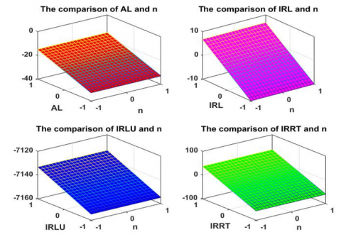
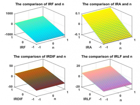
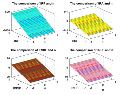
Figure 5. Graphical analysis for oxide network
Figure 6. Graphically analysis of honeycomb network
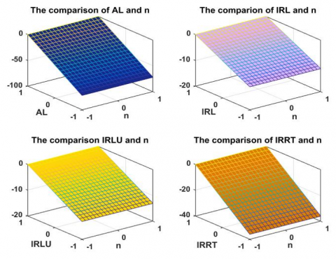
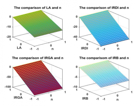
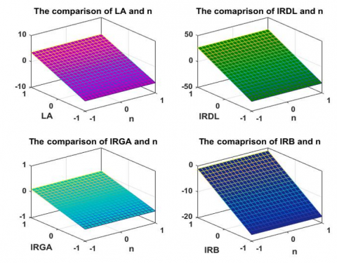
Figure 7. Graphically analysis of silicate network
Figure 8. Graphically analysis of chain silicate network
3.1 The numerical consequences and discussions
In this article, we've provided a visual examination of a few irregularity indices for the chemical framework. Figures 5-8 comparative analysis of AL(G), IRL(G), IRLU(G), IIRRT(G), IRF(G), IRA(G), IRDIF(G), IRLF(G), LA(G), IRDI(G), IRGA(G) and with different values of n for HCn, CSn, OXn and Sln.
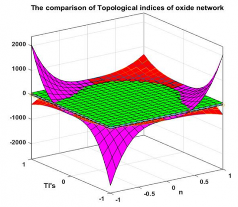
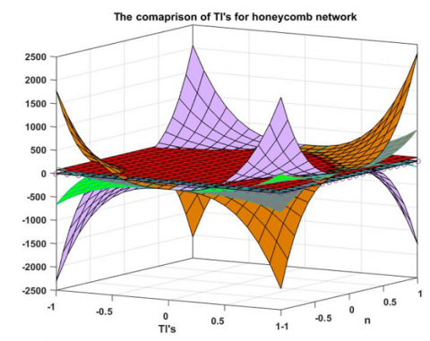
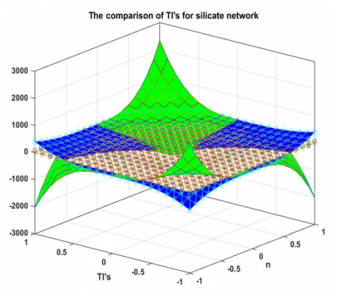
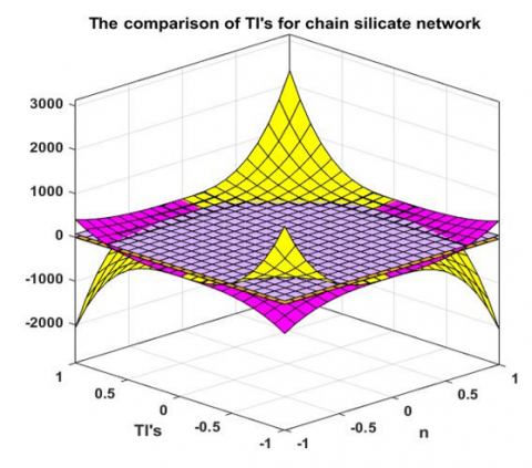
Figure 9. The comparison graphs of TI’s for the considered networks
The comparison of these topological indices allows for the assessment of molecular similarity or dissimilarity. Molecules with similar topological indices often exhibit similar behaviors, such as biological activity or chemical reactivity. This is particularly valuable in drug discovery and material design, where identifying structurally related compounds can guide research and development efforts. The preceding indices are extremely close at the commencement of the supplied domain eventually increasing rapidly. These include indices the index IRF(G) in oxide network, silicate network, and honeycomb In comparison to other indexes, the network has the greatest impact. As opposed to that, IRA(G) especially in comparison to other indexes, it rises steadily. The distance seen between indices in the oxide network IRA(G) and IRF(G) appeared at initial stage and it increase when the value of n increases. From Figure 9, it is easy to see that IRL(G), IRLF(G)and LA(G) are confide each other’s if oxide network, and the topological indices are close to each other. Similarly, for honeycomb network, silicate network, and for chain silicate network.
Throughout this research, we identified the degree-based topological indices of the relevant networks, such as the oxide network $\left(O X_n\right)$, honeycomb network $\left(H C_n\right)$, silicate network $\left(S L_n\right)$, and chain silicate network $\left(C S_n\right)$ and assessed their irregularity. The comparisons of 3D graphs are also depicted. Our results attract not only mathematician but also of theoretical chemists. The findings of this study can be used to analyze numerical quantities and further research to investigate a molecule's physical characteristics. As a result, it is a useful technique to eliminate costly and time-consuming laboratory studies. The distance-based topological indices, which are much more challenging and complex, can be used with the current methods. These types of studies will be the subject of future research.
[1] Balaban, A.T., Motoc, I., Bonchev, D., Mekenyan, O. (1983). Topological indices for structure-activity correlations. In Steric Effects in Drug Design. Topics in Current Chemistry, vol. 114. Springer, Berlin, Heidelberg. https://doi.org/10.1007/BFb0111212
[2] Balaban, A.T. (1988). Topological indices and their uses: A new approach for the coding of alkanes. Journal of Molecular Structure: THEOCHEM, 165(3-4): 243-253. https://doi.org/10.1016/0166-1280(88)87023-4
[3] Došlić, T., Réti, T., Vukičević, D. (2011). On the vertex degree indices of connected graphs. Chemical Physics Letters, 512(4-6): 283-286. https://doi.org/10.1016/j.cplett.2011.07.040
[4] Todeschini, R., Consonni, V. (2009). Molecular Descriptors for Chemoinformatics: Volume I: Alphabetical Listing/Volume II: Appendices, References. John Wiley & Sons.
[5] Refaee, E.A., Ahmad, A., Azeem, M. (2023). Sombor indices of γ-sheet of boron clusters. Molecular Physics, 121(15): e2214953. https://doi.org/10.1080/00268976.2023.2214953
[6] Ullah, A., Zeb, A., Zaman, S. (2022). A new perspective on the modeling and topological characterization of H-Naphtalenic nanosheets with applications. Journal of Molecular Modeling, 28(8): 211. https://doi.org/10.1007/s00894-022-05201-z
[7] Albertson, M.O. (1997). The irregularity of a graph. Ars Combinatoria, 46: 219-225.
[8] Gutman, I. (2018). Topological indices and irregularity measures. Bulletin of the International Mathematical Virtual Institute, 8: 469-475. https://doi.org/10.7251/BIMVI1803469G
[9] Abdo, H., Brandt, S., Dimitrov, D. (2014). The total irregularity of a graph. Discrete Mathematics Theoretical Computer Science, 16.
[10] Elphick, C., Wocjan, P. (2013). New measures of graph irregularity. arXiv preprint arXiv:1305.3570. https://doi.org/10.48550/arXiv.1305.3570
[11] Chartrand, G., Erdös, P., Oellermann, O.R. (1988). How to define an irregular graph. The College Mathematics Journal, 19(1): 36-42. https://doi.org/10.1080/07468342.1988.11973088
[12] Ahmad, A., Elahi, K., Azeem, M., Swaray, S., Asim, M.A. (2023). Topological descriptors for the metal organic network and its structural properties. Journal of Mathematics, 2022: 9859957. https://doi.org/10.1155/2022/9859957
[13] Ullah, A., Zaman, S., Hamraz, A., Muzammal, M. (2023). On the construction of some bioconjugate networks and their structural modeling via irregularity topological indices. The European Physical Journal E, 46(8): 72. https://doi.org/10.1140/epje/s10189-023-00333-3
[14] Dinar, J., Hussain, Z., Zaman, S., Rehman, S.U. (2023). Wiener index for an intuitionistic fuzzy graph and its application in water pipeline network. Ain Shams Engineering Journal, 14(1): 101826. https://doi.org/10.1016/j.asej.2022.101826
[15] Zaman, S., Jalani, M., Ullah, A., Saeedi, G. (2022). Structural analysis and topological characterization of sudoku nanosheet. Journal of Mathematics, 2022: 5915740. https://doi.org/10.1155/2022/5915740
[16] Wang, G., Yan, L., Zaman, S., Zhang, M. (2020). The connective eccentricity index of graphs and its applications to octane isomers and benzenoid hydrocarbons. International Journal of Quantum Chemistry, 120(18): e26334. https://doi.org/10.1002/qua.26334
[17] Dearden, J.C. (2017). The use of topological indices in QSAR and QSPR modeling. In Advances in QSAR Modeling. Challenges and Advances in Computational Chemistry and Physics, vol. 24. Springer, Cham. https://doi.org/10.1007/978-3-319-56850-8_2
[18] Zaman, S. (2021). Cacti with maximal general sum-connectivity index. Journal of Applied Mathematics and Computing, 65: 147-160. https://doi.org/10.1007/s12190-020-01385-w
[19] Vallet-Regí, M., Balas, F., Arcos, D. (2007). Mesoporous materials for drug delivery. Angewandte Chemie International Edition, 46(40): 7548-7558. https://doi.org/10.1002/anie.200604488
[20] Mandal, B., Chung, J.S., Kang, S.G. (2017). Exploring the geometric, magnetic and electronic properties of Hofmann MOFs for drug delivery. Physical Chemistry Chemical Physics, 19(46): 31316-31324. https://doi.org/10.1039/C7CP04831A
[21] Balaban, A.T. (1979). Chemical graphs: XXXIV. Five new topological indices for the branching of tree-like graphs [1]. Theoretica Chimica Acta, 53: 355-375. https://doi.org/10.1007/BF00555695
[22] Zaman, S., Ali, A. (2021). On connected graphs having the maximum connective eccentricity index. Journal of Applied Mathematics and Computing, 67: 131-142. https://doi.org/10.1007/s12190-020-01489-3
[23] Gutman, I. (2013). Degree-based topological indices. Croatica Chemica Acta, 86(4): 351-361. http://doi.org/10.5562/cca2294
[24] Ullah, A., Qasim, M., Zaman, S., Khan, A. (2022). Computational and comparative aspects of two carbon nanosheets with respect to some novel topological indices. Ain Shams Engineering Journal, 13(4): 101672. https://doi.org/10.1016/j.asej.2021.101672
[25] Wiener, H. (1947). Structural determination of paraffin boiling points. Journal of the American Chemical Society, 69(1): 17-20. https://doi.org/10.1021/ja01193a005
[26] Bollobás, B., Riordan, O. (2008). Random Graphs and Branching Processes. In Handbook of Large-Scale Random Networks. Bolyai Society Mathematical Studies, vol. 18. Springer, Berlin, Heidelberg. https://doi.org/10.1007/978-3-540-69395-6_1
[27] Zaman, S., He, X. (2022). Relation between the inertia indices of a complex unit gain graph and those of its underlying graph. Linear and Multilinear Algebra, 70(5): 843-877. https://doi.org/10.1080/03081087.2020.1749224
[28] Gross, J.L., Yellen, J. (Eds.). (2003). Handbook of Graph Theory. CRC Press.
[29] Temkin, O.N., Zeigarnik, A.V., Bonchev, D.G. (2020). Chemical Reaction Networks: A Graph-Theoretical Approach. CRC Press. https://doi.org/10.1201/9781003067887
[30] Zaman, S., Jalani, M., Ullah, A., Ali, M., Shahzadi, T. (2023). On the topological descriptors and structural analysis of cerium oxide nanostructures. Chemical Papers, 77(5): 2917-2922. https://doi.org/10.1007/s11696-023-02675-w
[31] Bharati Rajan, A.W., Grigorious, C., Stephen, S. (2012). On certain topological indices of silicate, honeycomb and hexagonal networks. Journal of Computer and Mathematical Sciences, 3(5): 498-556.
[32] Imran, M., Hayat, S., Mailk, M.Y.H. (2014). On topological indices of certain interconnection networks. Applied Mathematics and Computation, 244: 936-951. https://doi.org/10.1016/j.amc.2014.07.064
[33] Vukičević, D. (2009). On the edge degrees of trees. Glasnik Matematički, 44(2): 259-266. https://doi.org/10.3336/gm.44.2.01
[34] Li, X., Gutman, I., Randić, M. (2006). Mathematical aspects of Randić-type molecular structure descriptors. University, Faculty of Science.
[35] Réti, T., Sharafdini, R., Dregelyi-Kiss, A., Haghbin, H. (2018). Graph irregularity indices used as molecular descriptors in QSPR studies. MATCH Communications in Mathematicaland in Computer Chemistry, 79(2): 509-524.
[36] Ahmad, A. (2022). Computing the total vertex irregularity strength associated with zero divisor graph of commutative ring. Kragujevac Journal of Mathematics, 46(5): 711-719. https://doi.org/10.46793/KgJMat2205.711A
[37] Yu, X., Zaman, S., Ullah, A., Saeedi, G., Zhang, X. (2023). Matrix analysis of hexagonal model and its applications in global mean-first-passage time of random walks. IEEE Access, 11: 10045-10052. https://doi.org/10.1109/ACCESS.2023.3240468