Mohammed A. Jebur*![]() | Luay S. Alansari
| Luay S. Alansari
© 2023 IIETA. This article is published by IIETA and is licensed under the CC BY 4.0 license (http://creativecommons.org/licenses/by/4.0/).
OPEN ACCESS
Non-prismatic beams, which serve crucial roles in mechanical engineering applications, are subjected to both static and dynamic loads. Hence, their thorough analysis—particularly under free vibration—is of significant importance. This research undertakes an in-depth investigation into the free vibration characteristics of non-prismatic Euler-Bernoulli beams that exhibit linear variations in both width and height. These beams were studied under two distinct boundary conditions: simple support and clamped-clamped scenarios. The study's approach was twofold: analytical and numerical. The analytical method entailed computing the equivalent area and the equivalent second moment of area, thereby enabling an exploration of how variations in the second moment of inertia and cross-sectional area affect the natural frequencies and mode shapes of non-prismatic beams. Conversely, the numerical method employed the finite element method through ANSYS APDL software (version 17.2). The study's findings revealed that as the height and width of the beam decrease, natural frequencies decline and the maximum amplitude of the mode shapes escalates. It should be noted that the rate of decrease is more pronounced with changes in height than with alterations in width. Furthermore, the diminishing rate of natural frequencies and the decreasing maximum amplitude of the mode shape became more pronounced with the increase in mode number when the beam's height and width decreased. The results derived from the analytical procedure were validated against those from finite element analysis and other literature sources, demonstrating the reliability of the current method. The proposed analytical methodology, in its simplicity of use and accuracy, demonstrates considerable promise in comparison to numerical results.
free vibration, non-prismatic beam, ANSYS software, natural frequency, finite element method
Beams, integral structural constituents in numerous mechanical, civil, and architectural applications, provide essential support and stability. Non-prismatic beams, due to their superior strength and mass distribution compared to prismatic beams, are particularly adept at fulfilling specialized functional requirements in a range of sectors. These include architecture, rotor blades, aircraft wings, robotics, arch bridges, sports arenas, and other intriguing engineering applications.
Often, the unique demands of these applications necessitate the employment of beams with non-uniform cross-section areas and non-uniform material distribution along their length. This non-uniformity is leveraged to enhance key structural attributes such as buckling resistance, load capacity, and the fine-tuning of modal characteristics. Beams are subjected to a wide array of static and dynamic loads, and under certain conditions, the frequency of the dynamic load coincides with the beam's natural frequency. Consequently, resonance can cause the beam to vibrate until it fails.
Given its critical importance in diverse engineering fields, the vibration behavior of beams with non-uniform cross-section areas and material distribution has been a focal point in numerous research papers.
Several papers used the approximate solutions of partial differential equations to analyse the vibration behavior of non-prismatic beams. Each approximate solution made assumptions to overcome the nonlinearity generated in partial differential equations due to the change in geometry and material. Some of these approximate methods are the Frobeniucs method [1-7], Adomian decomposition method [8, 9], Galerkin method [10-12], finite element method [13-40], and Rayleigh-Ritz method [41-51].
The finite element technique was applied by Rossi and Laura [35] to simulate and investigate the dynamic behavior of the tapered homogeneous beams. Also, Alansari et al. [27] considered the finite element technique by using the ANSYS software to calculate the natural frequency of tapered cantilever beams. They studied the effect of the width ratio on the natural frequency ratio. Srikarrao et al. [28] calculated the natural frequency of the beam by employing the finite element technique and Regression method, and they compared the results of the two methods and found a good agreement between them.
In the same way, Jawad [29] applied the finite element technique to analyse the free vibration behavior of the tapered Euler-Bernoulli beam. He compared his results with those given in the available literature, and he found that the degree of flexural stiffness and tapered parameter causes decreasing in the natural frequency of tapered beams.
The Rayleigh-Ritz method was used in several studies involving non-prismatic beams. The Rayleigh-Ritz method was improved by Popplewell and Chang [47] by introducing discontinuities in the assumed deflection's second and third derivatives. Jaworski and Dowell [16] used the Rayleigh-Ritz method based on Bernoulli beam theory to study the free vibration behavior of multiple cross-section steps cantilevered beam. They compared their experimental results with theoretical results obtained by Rayleigh-Ritz and finite element methods. Alansari et al. [27, 32] applied the Classical Rayleigh and Modified Rayleigh methods to calculate the natural frequency of the tapered beam. They compared the results of natural frequency obtained by the Classical and Modified Rayleigh methods in addition to the finite element method (ANSYS software). Ghani et al. [52] used the classical Rayleigh method and modified the Rayleigh method to study the natural frequency of non-homogenous cantilever beams with square and circular cross-sections. They compared the natural frequencies obtained by classical and modified. They compared the results obtained by the Rayleigh method with those obtained by ANSYS software and discovered that the classical Rayleigh method and ANSYS had a good agreement for regions with lengths greater than half the beam length and an excellent agreement for regions with lengths less than half the beam length.
In previous papers, special cases of non-prismatic beams were studied. In other words, no general solution for non-prismatic beams was presented in previous literature. Currently, there are no reliable analytical methods for solving linear differential equations with variable coefficients.
In this work, analytical and numerical methods were used to calculate the natural frequencies of non-prismatic beams with linear changes in height, width, and both height and width simultaneously. The analytical method is based on the calculation of equivalent area and equivalent second moment of area and then applying these equivalent values to the solution of the Euler–Bernoulli equation in order to find general solution of non-prismatic beams. The new analytical method is simple and agrees well with the numerical results. The major contribution of this study is a simple solution to free vibration of non-prismatic beam using the equivalent second moment of area approach. The numerical method is based on the finite element method using ANSYS APDL version 17.2.
This paper is organized into the following sections: In Section 2, the basic mathematical equations of dimensions for non-prismatic beams are described. In Section 3, the natural frequency equations of uniform beams based on Euler–Bernoulli beam theory are displayed. In Section 4, the calculating methods of equivalent area and equivalent second moment of area of non-prismatic beams are illustrated. The finite element model is described in Section 5. The accuracy of the present methods is checked in Section 6. Finally, the results and conclusions are displayed in Sections 7 and 8.
The homogenous beam with a linear and nonlinear variation of cross-section area along the beam length is used in this work. The linear variation of the cross-section area is done by assuming the linear variation of width (b) or height (or thickness) (h) of the beam according to the following equations (see Figure 1):
$b(x)=b_0\left(1+\alpha_b *\left(\frac{x}{L}\right)\right)$ (1)
$h(x)=h_0\left(1+\alpha_h *\left(\frac{x}{L}\right)\right)$ (2)
Here: $\alpha_b=\left(\frac{b_0}{b_1}\right)-1 ; \alpha_h=\left(\frac{h_0}{h_1}\right)-1$.
According to Eq. (1) and Eq. (2), the variation of cross-section area (A(x)) is linear too.
Figure 1. The dimensions of the non-prismatic beam
$A(x)= \begin{cases}h_0 * b_0\left(1+\alpha_b *\left(\frac{x}{L}\right)\right) & \text { constant height } \\ b_0 * h_0\left(1+\alpha_h *\left(\frac{x}{L}\right)\right) & \text { constant width }\end{cases}$ (3)
While the variation of second moment of area (I(x)) is linear when the height of beam is constant and nonlinear when the width of beam is constant, it can be described as:
$I(x)=\left\{\begin{array}{l}b_0\left(1+\alpha_b *\left(\frac{x}{L}\right)\right) *\left(h_0\right)^3 / 12 \text { constant height } \\ b_0 *\left(h_0\left(1+\alpha_h *\left(\frac{x}{L}\right)\right)\right)^3 / 12 \text { constant width }\end{array}\right.$ (4)
On other side, when the width and height are changed together, the cross-section and the second moment of area are:
$A(x)=b_0\left(1+\alpha_b *\left(\frac{x}{L}\right)\right) * h_0\left(1+\alpha_h *\left(\frac{x}{L}\right)\right)$ (5)
$I(x)=b_0\left(1+\alpha_b *\left(\frac{x}{L}\right)\right) *\left(h_0\left(1+\alpha_h *\left(\frac{x}{L}\right)\right)\right)^3 / 12$ (6)
As shown in Eqs. (3)-(6), the cross-section area changes linearly when the width and height of the beam are changed separately, and if the width and height of the beam vary together, the cross-section area changes nonlinearly. At the same time, the second moment of the area changes linearly if the width of the beam changes only. The linear and nonlinear variation in the second moment of area and cross-section area affect the free vibration behavior of the beam that is described by the following partial differential equation [53-55]:
$\frac{\partial^2}{\partial x^2}\left(E I(x) \frac{\partial^2 w}{\partial x^2}\right)+\rho A(x) \frac{\partial^2 w}{\partial t^2}=0$ (7)
From Eq. (7), the variation in the second moment of area and cross-section area greatly affects the natural frequency and mode shape.
For uniform and homogenous beams, the analytical solutions of the partial differential equation (Eq. (7)) with various boundary conditions are found in vibration textbooks [53-55]. The analytical solutions found the values of natural frequencies and mode shapes, and equations that describe natural frequencies and mode shapes with various boundary conditions are shown in studies [53-55].
3.1 Simply supported beam
The natural frequency equation is [53]:
$\omega_i=\left(\beta_i l\right)^2 \sqrt{\frac{E I}{\rho A l^4}}=\left(i^2 \pi^2\right)^2 \sqrt{\frac{E I}{\rho A l^4}},(\mathrm{i}=1,2, \ldots)$ (8)
3.2 Clamp-Clamp beam
The natural frequency equation is [53]:
$\omega_i=\left(\beta_i l\right)^2\left(\frac{E I}{\rho A l^4}\right)^{1 / 2}, \cos \beta_i l \cosh \beta_i l-1=0,(\mathrm{i}=1,2, \ldots)$ (9)
This work suggests a new simple analytical solution for the free vibration problem of non-prismatic homogeneous beams. The new solution is based on the analytical solution for the free vibration problem of a uniform homogeneous beam. It uses the equivalent cross-section area and second moment of area to overcome the problem of the non-prismatic beam.
4.1 Equivalent cross area
In order to overcome the change in cross-section are the equivalent cross-area of the non-prismatic beam is calculated by the following equation:
$A_{\text {eq }}=(A(0)+A(L)) / 2$ (10)
4.2 Equivalent second moment of area
In order to calculate the equivalent second moment of area, the non-prismatic beam is divided into (n) parts (i.e. (M=N+1) points), and each part has uniform cross-section area and uniform second moment of area using the following equation:
$I_n=\frac{b_n *\left(h_n\right)^3}{12}, \mathrm{n}=1,2,3 \ldots \mathrm{N}$ (11)
Here: $h_n=\left(h_m+h_{m+1}\right) / 2$ (New height of part);
$b_n=\left(b_m+b_{m+1}\right) / 2$ (New width of part)
According to Eq. (11), the non-prismatic beam now appears as a stepped beam (see Figure 2).
For clamp-free non-prismatic beam, the equivalent second moment of the area can be calculated as [27, 32, 52]:
$(I)_{e q}=\frac{\left(L_{\text {total }}\right)^3}{\sum_{n=1}^N \frac{\left(L_n\right)^3-\left(L_{n-1}\right)^3}{(I)_n}}$ (12)
For simply supported or clamp-clamp non-prismatic beam, the equivalent second moment of the area can be calculated according to the following four steps:
$\bar{X}=\frac{\sum V * \bar{x}}{\sum V}$ (13)
Here: $\mathrm{V}=b_n * h_n * \Delta x ; \Delta x=L / N$
Figure 2. Non-prismatic beam transfers into stepped beam
Figure 3. Configuration of stepped S-S&C-C beam
$\left(I_{e q}\right)_L=\frac{L_L{ }^3}{\sum_{n=1}^{N_{L e f t} \frac{l_n{ }^3-l_{n-1}{ }^3}{I_n}}}$ (14)
$\left(I_{e q}\right)_R=\frac{\left(L_R\right)^3}{\sum_{n=1}^{N_{R i g h t}} \frac{l_{n-1}{ }^3-l_n{ }^3}{I_n}}$ (15)
EThe equivalent second moment of area of S-S and C-C stepped beam is calculated by:
$I_{e q}=\frac{\left(L_R+L_L\right) *\left(L_R\right)^2 *\left(L_L\right)^2}{\left(\left(\sum_{n=1}^{N_{R i g h t}} \frac{l_{n-1}{ }^3-l_n{ }^3}{I_n}\right) * L_R{ }^2\right)+\left(\left(\sum_{n=1}^{N_{L e f t}} \frac{l_n{ }^3-l_{n-1}{ }^3}{I_n}\right) * L_L{ }^2\right)}$ (16)
The model was created using finite elements. Using ANSYS APDL version 17.2. The non-prismatic beam was drawn using 18 key points (9 at each end face), as shown in Figure 4-a. These key points are connected using lines (see Figure 4-b), and these lines are used to generate four solid bodies (see Figure 4-c). In the ANSYS model, the element SOLID187 is used to mesh the four bodies after gluing them. The properties of the SOLID187 are: "SOLID187 element is a higher-order 3-D, 10-node element. SOLID187 has a quadratic displacement behavior and is well suited to modeling irregular meshes (such as those produced by various CAD/CAM systems). The element is defined by 10 nodes with three degrees of freedom at each node: translations in the directions of the nodal x, y, and z. The element has plasticity, hyperelasticity, creep, stress stiffening, large deflection, and large strain capabilities. It also has mixed formulation capability to simulate deformations of nearly incompressible elastoplastic and fully incompressible hyperelastic materials.” [56, 57] (See Figure 5).
(a) Keypoints of face ends
(b) Lines links to keypoints
(c) Solid bodies are generated by lines
Figure 4. The geometry of non-prismatic beam
Figure 5. The meshing of the non-prismatic beam with SOLID187
In order to check the validity of the present work (i.e., analytical and numerical methods), the comparison between the dimensionless natural frequency results of the analytical and numerical methods and those obtained in the literature. The dimensionless natural frequency is shown in the study [58]:
$\bar{\omega}_i=\omega_i \sqrt{\frac{\rho A(0) L^4}{E I(0)}} \quad i=1,2,3, \ldots$ (17)
6.1 Simply supported tapered beam
Table 1. Validation results of dimensionless natural frequencies of S-S supported tapered beam
|
ah |
Methods |
Dimensionless Natural Frequency |
||
|
n=1 |
n=2 |
n=3 |
||
|
0.1 |
This work |
9.3823 |
37.5291 |
84.4405 |
|
ANSYS |
9.3358 |
36.9451 |
81.6550 |
|
|
Ref. [58] |
9.3651 |
37.4459 |
84.1401 |
|
|
Ref. [59] |
9.3675 |
37.4840 |
84.3350 |
|
|
Ref. [60] |
9.3675 |
37.4843 |
84.3347 |
|
|
0.5 |
This work |
7.3524 |
29.4095 |
66.1713 |
|
ANSYS |
7.1081 |
28.7106 |
63.7571 |
|
|
Ref. [58] |
7.1197 |
28.9219 |
64.8260 |
|
|
Ref. [59] |
7.1215 |
28.9520 |
64.9790 |
|
|
Ref. [60] |
7.1210 |
28.9496 |
64.9737 |
|
|
0.9 |
This work |
4.7327 |
18.9307 |
42.5941 |
|
ANSYS |
3.8879 |
18.0773 |
45.6756 |
|
|
Ref. [58] |
3.8886 |
18.1030 |
39.9008 |
|
|
Ref. [59] |
3.8895 |
18.1230 |
40.0110 |
|
|
Ref. [60] |
3.8831 |
18.0964 |
39.9458 |
|
Table 2. Validation results of dimensionless natural frequencies of C-C tapered beam
|
ah |
Methods |
Dimensionless Natural Frequency |
||
|
n=1 |
n=2 |
n=3 |
||
|
0.1 |
This work |
21.2515 |
58.5804 |
114.8411 |
|
ANSYS |
21.0275 |
56.8848 |
108.8761 |
|
|
Ref. [58] |
21.2343 |
58.4803 |
114.4860 |
|
|
Ref. [59] |
21.2410 |
58.5500 |
114.7800 |
|
|
Ref. [60] |
21.2411 |
58.5503 |
114.7810 |
|
|
0.5 |
This work |
16.6536 |
45.9062 |
89.9945 |
|
ANSYS |
16.2712 |
44.2939 |
85.5112 |
|
|
Ref. [58] |
16.3343 |
44.9375 |
87.9316 |
|
|
Ref. [59] |
16.3360 |
44.9810 |
88.1380 |
|
|
Ref. [60] |
16.3382 |
44.9879 |
88.1527 |
|
|
0.9 |
This work |
10.7198 |
29.5495 |
57.9290 |
|
ANSYS |
9.9210 |
26.9871 |
52.3659 |
|
|
Ref. [58] |
9.93327 |
27.1150 |
52.8293 |
|
|
Ref. [59] |
9.8846 |
27.0080 |
52.7080 |
|
|
Ref. [60] |
9.91912 |
27.1025 |
52.8897 |
|
Table 1 compares the dimensionless natural frequencies results of the analytical and numerical methods and that obtained in Nikolić and Šalinić [58], Wang and Wang [59]. Furthermore, Wu [60] simply supported a tapered beam for different values of ah. From Table 1, there is a very good agreement between the present methods (analytical and numerical methods) and that obtained in Nikolić et al. [58], Wang and Wang [59] and Wu [60] in the second natural frequency when ah=0.1 and 0.5 when ah=0.9.
The first natural frequency obtained by the present analytical method is greater than other values. At the same time, the third natural frequency obtained by the present numerical method is smaller than other values for all values of ah. When ah=0.1 and 0.5, there is a very good agreement between the present methods (analytical and numerical methods) and that obtained in Nikolić et al. [58], Wang and Wang [59] and Wu [60] in the first and second natural frequencies. When ah=0.9, the first natural frequency obtained by the present analytical and numerical method is greater than other values.
6.2 Clamp-clamp tapered beam
Table 2 compares the dimensionless natural frequencies results of the analytical and numerical methods obtained in Nikolić et al. [58], Wang and Wang [59] and Wu [60] for the clamp-clamp tapered beam for different values of ah.
In this work, three main cases were considered to study the effect of linear variation in dimensions on the natural frequencies of tapered beams. The tapered beam has a modulus of elasticity (200 GPa), Poisson's Ratio (0.3), and density (7,800 kg/m3). The length of the tapered beam is (1 m), and the height and width of the tapered beam at x=0 are (0.05 m). The three cases are:
7.1 Case one: Height variation
In this case, the change in the second moment of area and cross-section area is illustrated in Figure 6. The cross-section area of the tapered beam decreases linearly (the decreasing rate of cross-section area=ah, see Eq. (3)), while the second-moment area decreases at a rate larger than that of the cross-section area (see Eq. (4)). The natural frequencies will also change according to these changes in the second moment of area and cross-section area.
Figure 7 compares the analytical and numerical results of C-C and S-S tapered height beams for the first, second, and third natural frequencies. When (ah) decreases, the second moment of area and cross-section area decreases too, and in Figure 6, the decreasing rate of the second moment of area is greater than that of the cross-section area. Therefore, the dimensionless frequencies will decrease (see Eqs. (8) and (9)), and the decreasing rates of dimensionless frequencies will increase with increasing the mode number.
Also, the agreement between analytical and numerical results decreases with decreasing (ah) and increasing the mode number. The absolute discrepancy percentages between numerical and analytical results were (13.64, 5, and 6.9%) for the first, second, and third natural frequencies of S-S tapered beams, respectively. For C-C tapered beams, the absolute discrepancy percentage between numerical and analytical results were (6.7, 7.96, and 9.1%) for first, second, and third natural frequencies.
(a) Area
(b) Second moment of area
Figure 6. Area and second moment of area variation with (ah)
(a) 1st frequency of C-C
(b) 1st frequency of S-S
(c) 2nd frequency of C-C
(d) 2nd frequency of S-S
(e) 3rd frequency of C-C
(f) 3rd frequency of S-S
Figure 7. First three dimensionless natural frequencies of C-C and S-S tapered beams with different values of (ah)
7.2 Case two: Width variation
In this case, the change in the second moment of area and cross-section area is illustrated in Figure 8. The cross-section area and second-moment area of the tapered beam decrease linearly at the same rate (ab) (see Eqs. (3) and (4)), and According to these changes in the second moment of area and cross-section area, the natural frequencies will change too.
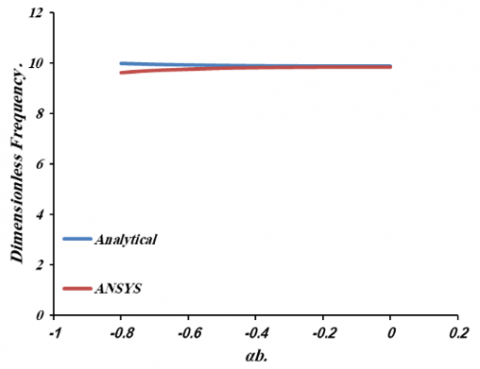
The comparison between the analytical and numerical results of C-C and S-S tapered width beams for the first, second, and third natural frequencies is illustrated in Figure 9.
The second moment of area and cross-section area decrease when (ab) decreases. The decreasing rate of the second moment of area is the same as the cross-section area and equals (ab) according to Figure 8. Therefore, the dimensionless frequencies are constant or slightly varied when (ab) decreases for the three model numbers (see Eqs. (8) and (9)). Also, the agreement between analytical and numerical results decreases with decreasing (ab) and increasing the mode number. The absolute discrepancy percentages between numerical and analytical results were (6.8, 7, and 8%) for the first, second, and third natural frequencies of C-C tapered beams, respectively. For S-S tapered beams, the absolute discrepancy percentage between numerical and analytical results were (3.8, 2.76, and 4.8%) for first, second, and third natural frequencies.
7.3 Case three: Width and height variation
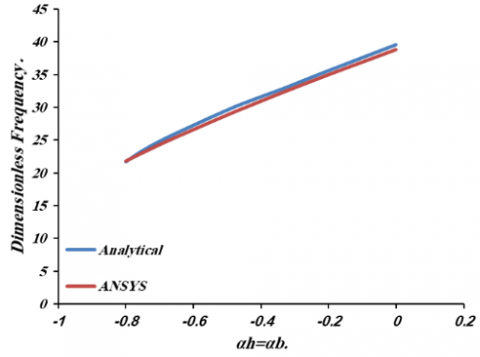
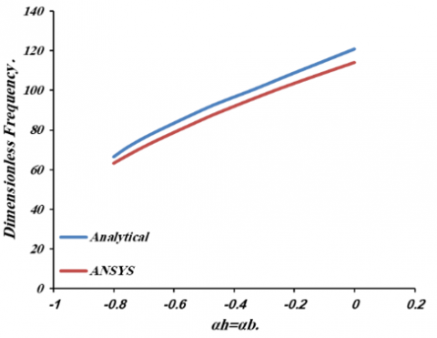
In this case, the change in the second moment of area and cross-section area are shown in Figure 10. The cross-section area of the tapered beam decreases (see Eq. (3)) while the second-moment area decreases at a rate larger than that of the cross-section area (see Eq. (4)). According to these changes in the second moment of area and cross-section area, the natural frequencies will change too (see Eqs. (8) and (9)). Figure 11 compares the analytical and numerical natural frequencies when the height and width are decreased together.
Conversely, the agreement between analytical and numerical results decreases with a decrease (ah), (ab), and an increasing the mode number. The absolute discrepancy percentages between numerical and analytical results were (2.17, 4.3, and 6.1%) for the first, second, and third natural frequencies of C-C tapered beams, respectively. For S-S tapered beams, the absolute discrepancy percentages between numerical and analytical results were (14, 2.4, and 4%) for first, second, and third natural frequencies, respectively.
Figures 7, 9, and 11, the ab effect is small, approximately zero compared with the ah effect, but the ab effect appears when ab and ah are varied together.
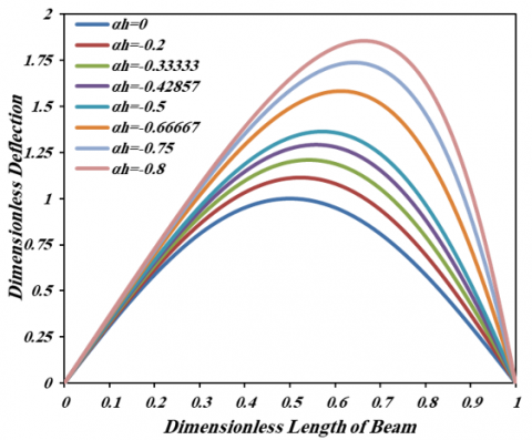
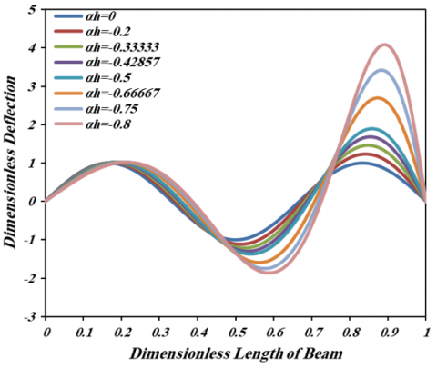
Finally, Figures 12, 13, and 14 depict the three dimensionless mode shapes of the non-prismatic beam at the clamped-clamped and simply supported boundary conditions for various (ah, ab and ah=ab) value from ANSYS APDL. The maximum amplitude of the mode shapes increases as the values of (ah, ab and ah=ab) for each case decrease.
(a) Area.
(b) Second moment of area
Figure 8. Area and second moment of area variation with (ab)
(a) 1st frequency of C-C
(b) 1st frequency of S-S
(c) 2nd frequency of C-C
(d) 2nd frequency of S-S
(e) 3rd of C-C
(f) 3rd frequency of S-S
Figure 9. First three dimensionless natural frequencies of C-C and S-S tapered beams with different values of (ab)
(a) Area
(b) Second moment of area
Figure 10. Area and second moment of area variation with (ab=ab)
(a) 1st frequency of C-C
(b) 1st frequency of S-S
(c) 2nd of C-C
(d) 2nd frequency of S-S
(e) 3rd frequency of C-C
(f) 3rd frequency of S-S
Figure 11. First three dimensionless natural frequencies of C-C and S-S tapered beams with different values of (ah=ab)
(a) Mode shape1 of C-C
(b) Mode shape1 of S-S
(c) Mode shape2 of C-C
(d) Mode shape2 of S-S
(e) Mode shape3 of C-C
(f) Mode shape3 of S-S
Figure 12. The first three dimensionless mode shapes of C-C and S-S tapered beams with different values of (ah)
(a) Mode shape1 of C-C
(b) Mode shape1 of S-S
(c) Mode shape2 of C-C
(d) Mode shape2 of S-S
(e) Mode shape3 of C-C
(f) Mode shape3 of S-S
Figure 13. The first three dimensionless mode shapes of C-C and S-S tapered beams with different values of (ab)
(a) Mode shape1 of C-C
(b) Mode shape1 of S-S
(c) Mode shape2 of C-C
(d) Mode shape2 of S-S
(e) Mode shape3 of C-C
(f) Mode shape3 of S-S
Figure 14. The first three dimensionless mode shapes of C-C and S-S tapered beams with different values of (ah=ab)
This study introduces a novel analytical method to compute the natural frequencies of Simply Supported (S-S) and Clamped-Clamped (C-C) tapered beams. This innovative approach considers the equivalent cross-section and equivalent second moment of area, applying these values to the solution of uniform beam free vibration behavior based on Euler-Bernoulli's theory. Concurrently, a 3D model was constructed using the finite element technique in ANSYS APDL Version 17.2. The investigation led us to the following conclusions:
In future work, this new analytical method will be utilized to analyze the impact of nonlinear variation on the natural frequencies and mode shape under various boundary conditions.
|
bo |
The width of the beam at x=0 |
|
ho |
The height (or thickness) of the beam at x=0 |
|
b1 |
The width of the beam at x=L |
|
ho |
The height (or thickness) of the beam at x=L |
|
b(x) |
The width of the beam at any x |
|
h(x) |
The height (or thickness) of the beam at any x |
|
L |
The length of a beam |
|
hn |
A new height of a part |
|
bn |
New width of a part |
|
Greek symbols |
|
|
ab |
The rate of variation of the width of the beam |
|
aa |
The rate of variation of the height (or thickness) of the beam |
|
Subscripts |
|
|
S-S |
Simply supported |
|
C-C |
Clamp-clamp |
[1] Naguleswaran, S. (1992). Vibration of an Euler-Bernoulli beam of constant depth and with linearly varying breadth. Journal of Sound and Vibration, 153(3): 509-522. https://doi.org/10.1016/0022-460X(92)90379-C
[2] Naguleswaran, S. (1994). A direct solution for the transverse vibration of Euler-Bernoulli wedge and cone beams. Journal of Sound and Vibration, 172(3): 289-304. https://doi.org/10.1006/jsvi.1994.1176
[3] Naguleswaran, S. (1994). Vibration in the two principal planes of a non-uniform beam of rectangular cross-section, one side of which varies as the square root of the axial co-ordinate. Journal of Sound and Vibration, 172(3): 305-319. http://dx.doi.org/10.1006/jsvi.1994.1177
[4] Chaudhari, T.D., Maiti, S.K. (1999). Modelling of transverse vibration of beam of linearly variable depth with edge crack. Engineering Fracture Mechanics, 63(4): 425-445. https://doi.org/10.1016/s0013-7944(99)00029-6
[5] Wang, G., Wereley, N.M. (2003). Free vibration analysis of rotating blades with uniform tapers. In ASME International Mechanical Engineering Congress and Exposition, 37122: 1073-1084. https://doi.org/10.1115/IMECE2003-43636
[6] Banerjee, J.R. (2006). Free vibration of a composite Timoshenko beam using the dynamic stiffness method. Civil-Comp Proceedings, 83: 1034-1054. https://doi.org/10.4203/ccp.83.28
[7] Firouz-Abadi, R.D., Rahmanian, M., Amabili, M. (2013). Exact solutions for free vibrations and buckling of double tapered columns with elastic foundation and tip mass. Journal of Vibration and Acoustics, 135(5): 051017. https://doi.org/10.1115/1.4023991
[8] Hsu, J.C., Lai, H.Y., Chen, C.O.K. (2008). Free vibration of non-uniform Euler–Bernoulli beams with general elastically end constraints using Adomian modified decomposition method. Journal of Sound and Vibration, 318(4-5): 965-981. https://doi.org/10.1016/j.jsv.2008.05.010
[9] Mao, Q., Pietrzko, S. (2012). Free vibration analysis of a type of tapered beams by using Adomian decomposition method. Applied Mathematics and Computation, 219(6): 3264-3271. https://doi.org/10.1016/j.amc.2012.09.069
[10] Huo, Y., Wang, Z. (2016). Dynamic analysis of a rotating double-tapered cantilever Timoshenko beam. Archive of Applied Mechanics, 86: 1147-1161. https://doi.org/10.1007/s00419-015-1084-6
[11] Navadeh, N., Hewson, R.W., Fallah, A.S. (2018). Dynamics of transversally vibrating non-prismatic Timoshenko cantilever beams. Engineering Structures, 166: 511-525. http://dx.doi.org/10.1016/j.engstruct.2018.03.088
[12] Domagalski, Ł. (2021). Comparison of the natural vibration frequencies of timoshenko and bernoulli periodic beams. Materials, 14(24): 7628. https://doi.org/10.3390/ma14247628
[13] Hirst, M.J.S., Yeo, M.F. (1980). The analysis of composite beams using standard finite element programs. Computers & Structures, 11(3): 233-237. https://doi.org/10.1016/0045-7949(80)90163-7
[14] Karabalis, D.L., Beskos, D.E. (1983). Static, dynamic and stability analysis of structures composed of tapered beams. Computers & Structures, 16(6): 731-748. https://doi.org/10.1016/0045-7949(83)90064-0
[15] Schnabl, S., Saje, M., Turk, G., Planinc, I. (2007). Locking-free two-layer Timoshenko beam element with interlayer slip. Finite Elements in Analysis and Design, 43(9): 705-714. https://doi.org/10.1016/j.finel.2007.03.002
[16] Jaworski, J.W., Dowell, E.H. (2008). Free vibration of a cantilevered beam with multiple steps: Comparison of several theoretical methods with experiment. Journal of Sound and Vibration, 312(4-5): 713-725. https://doi.org/10.1016/j.jsv.2007.11.010
[17] Yardimoglu, B. (2010). A novel finite element model for vibration analysis of rotating tapered Timoshenko beam of equal strength. Finite Elements in Analysis and Design, 46(10): 838-842. https://doi.org/10.1016/j.finel.2010.05.003
[18] Attarnejad, R., Semnani, S.J., Shahba, A. (2010). Basic displacement functions for free vibration analysis of non-prismatic Timoshenko beams. Finite Elements in Analysis and Design, 46(10): 916-929. https://doi.org/10.1016/j.finel.2010.06.005
[19] Shooshtari, A., Khajavi, R. (2010). An efficient procedure to find shape functions and stiffness matrices of nonprismatic Euler–Bernoulli and Timoshenko beam elements. European Journal of Mechanics-A/Solids, 29(5): 826-836. https://doi.org/10.1016/j.euromechsol.2010.04.003
[20] Alshorbagy, A.E., Eltaher, M.A., Mahmoud, F. (2011). Free vibration characteristics of a functionally graded beam by finite element method. Applied Mathematical Modelling, 35(1): 412-425. https://doi.org/10.1016/j.apm.2010.07.006
[21] Attarnejad, R., Shahba, A., Eslaminia, M. (2011). Dynamic basic displacement functions for free vibration analysis of tapered beams. Journal of Vibration and Control, 17(14): 2222-2238. http://dx.doi.org/10.1177/1077546310396430
[22] Attarnejad, R., Shahba, A., Semnani, S.J. (2011). Analysis of non-prismatic Timoshenko beams using basic displacement functions. Advances in Structural Engineering, 14(2): 319-332. https://doi.org/10.1260/1369-4332.14.2.319
[23] Zona, A., Ranzi, G. (2011). Finite element models for nonlinear analysis of steel–concrete composite beams with partial interaction in combined bending and shear. Finite Elements in Analysis and Design, 47(2): 98-118. https://doi.org/10.1016/j.finel.2010.09.006
[24] Chakrabarti, A., Sheikh, A.H., Griffith, M., Oehlers, D.J. (2012). Analysis of composite beams with partial shear interactions using a higher order beam theory. Engineering Structures, 36: 283-291. https://doi.org/10.1016/j.engstruct.2011.12.019
[25] Kuo, Y.H., Wu, T.H., Lee, S.Y. (1992). Bending vibrations of a rotating non-uniform beam with tip mass and an elastically restrained root. Computers & Structures, 42(2): 229-236. https://doi.org/10.1016/0045-7949(92)90206-F
[26] He, P., Liu, Z., Li, C. (2013). An improved beam element for beams with variable axial parameters. Shock and Vibration, 20(4): 601-617. https://doi.org/10.3233/SAV-130771
[27] Alansari, L.S., Al-Hajjar, A.M., Husam Jawad, A. (2018). Calculating the natural frequency of cantilever tapered beam using classical Rayleigh, modified Rayleigh and finite element methods. International Journal of Engineering & Technology, 7(4): 4866-4872. https://doi.org/10.14419/ijet.v7i4.25334
[28] Srikarrao, C., Kumar, K., Kumar, P.P., Mukul, C., Vinay, P. (2016). Structural dynamic reanalysis of cantilever beam using polynomial regression method. IOSR Journal of Mechanical and Civil Engineering (IOSR-JMCE), 13(5): 1-14. https://doi.org/10.9790/1684-1305050114
[29] Jawad, D.H. (2013). Free vibration and buckling behavior of tapered beam by finite element method. Journal of Babylon University/Engineering Sciences, 21(3): 1043-1051. https://iasj.net/iasj/article/78075
[30] Uddin, M.A., Sheikh, A.H., Brown, D., Bennett, T., Uy, B. (2017). A higher order model for inelastic response of composite beams with interfacial slip using a dissipation based arc-length method. Engineering Structures, 139: 120-134. https://doi.org/10.1016/j.engstruct.2017.02.025
[31] Zappino, E., Viglietti, A., Carrera, E. (2018). Analysis of tapered composite structures using a refined beam theory. Composite Structures, 183: 42-52. https://doi.org/10.1016/j.compstruct.2017.01.009
[32] Alansari, L.S., Zainy, H.Z., Yaseen, A.A., Aljanabi, M. (2019). Calculating the natural frequency of hollow stepped cantilever beam. International Journal of Mechanical Engineering and Technology (IJMET), 10(1): 898-914.
[33] Shen, Y., Zhu, Z., Wang, S., Wang, G. (2019). Dynamic analysis of tapered thin-walled beams using spectral finite element method. Shock and Vibration, 2019: 2174209. https://doi.org/10.1155/2019/2174209
[34] Bazoune, A., Khulief, Y.A. (1992). A finite beam element for vibration analysis of rotating tapered Timoshenko beams. Journal of Sound and Vibration, 156(1): 141-164. https://doi.org/10.1016/0022-460X(92)90817-H
[35] Rossi, R.E., Laura, P.A.A. (1993). Numerical experiments on vibrating, linearly tapered timoshenko beans. Journal of Sound Vibration, 168(1): 179-183. https://doi.org/10.1006/jsvi.1993.1398
[36] Salari, M.R., Spacone, E., Shing, P.B., Frangopol, D.M. (1998). Nonlinear analysis of composite beams with deformable shear connectors. Journal of Structural Engineering, 124(10): 1148-1158. https://doi.org/10.1061/(asce)0733-9445(1998)124:10(1148)
[37] Rao, S.S., Gupta, R.S. (2001). Finite element vibration analysis of rotating Timoshenko beams. Journal of Sound and Vibration, 242(1): 103-124. https://doi.org/10.1006/jsvi.2000.3362
[38] Keller, T., Tirelli, T., Zhou, A. (2005). Tensile fatigue performance of pultruded glass fiber reinforced polymer profiles. Composite Structures, 68(2): 235-245. https://doi.org/10.1016/j.compstruct.2004.03.021
[39] Yardimoglu, B. (2006). Vibration analysis of rotating tapered Timoshenko beams by a new finite element model. Shock and Vibration, 13(2): 117-126. https://doi.org/10.1155/2006/283150
[40] Vo, T.P., Lee, J. (2007). Flexural–torsional behavior of thin-walled closed-section composite box beams. Engineering Structures, 29(8): 1774-1782. https://doi.org/10.1016/j.engstruct.2006.10.002
[41] Downs, B. (1978). Reference frequencies for the validation of numerical solutions of transverse vibrations of non-uniform beams. Journal of Sound and Vibration, 61(1): 71-78. https://doi.org/10.1016/0022-460X(78)90042-1
[42] Kim, C.S., Dickinson, S.M. (1989). On the analysis of laterally vibrating, elastically supported, slender beams. Journal of Sound Vibration, 129(1): 161-165. http://dx.doi.org/10.1016/0022-460X(89)90543-9
[43] Ansari, R., Sahmani, S., Rouhi, H. (2011). Rayleigh–Ritz axial buckling analysis of single-walled carbon nanotubes with different boundary conditions. Physics Letters A, 375(9): 1255-1263. https://doi.org/10.1016/j.physleta.2011.01.046
[44] Yuan, J., Dickinson, S.M. (1992). On the use of artificial springs in the study of the free vibrations of systems comprised of straight and curved beams. Journal of Sound and Vibration, 153(2): 203-216. https://doi.org/10.1016/S0022-460X(05)80002-1
[45] Lee, H.P., Ng, T.Y. (1994). Vibration and buckling of a stepped beam. Applied Acoustics, 42(3): 257-266. https://doi.org/10.1016/0003-682X(94)90113-9
[46] Liu, W.K., Jun, S., Li, S., Adee, J., Belytschko, T. (1995). Reproducing kernel particle methods for structural dynamics. International Journal for Numerical Methods in Engineering, 38(10): 1655-1679. https://doi.org/10.1002/nme.1620381005
[47] Popplewell, N., Chang, D. (1996). Free vibrations of a complex Euler-Bernoulli beam. Journal of Sound and Vibration, 190(5): 852-856. https://doi.org/10.1006/jsvi.1996.0098
[48] Banerjee, J. (2000). Free vibration of centrifugally stiffened uniform and tapered beams using the dynamic stiffness method. Journal of Sound and Vibration, 233(5): 857-875. https://doi.org/10.1006/jsvi.1999.2855
[49] Attarnejad, R., Manavi, N., Farsad, A. (2006). Exact solution for the free vibration of a tapered beam with elastic end rotational restraints. In Computational Methods, pp. 1993-2003. Springer, Netherlands. https://doi.org/10.1007/978-1-4020-3953-9_146
[50] Bazoune, A. (2007). Effect of tapering on natural frequencies of rotating beams. Shock and Vibration, 14(3): 169-179. https://doi.org/10.1155/2007/865109
[51] Ece, M.C., Aydogdu, M., Taskin, V. (2007). Vibration of a variable cross-section beam. Mechanics Research Communications, 34(1): 78-84. https://doi.org/10.1016/j.mechrescom.2006.06.005
[52] Ghani, S.N., Neamah, R.A., Abdalzahra, A.T., Al-Ansari, L.S., Abdulsamad, H.J. (2022). Analytical and numerical investigation of free vibration for stepped beam with different materials. Open Engineering, 12(1): 184-196. https://doi.org/10.1515/eng-2022-0031
[53] Rao, S.S. (2019). Vibration of Continuous Systems. John Wiley & Sons.
[54] Bhave, S. (2010). Mechanical Vibrations. Pearson Education, India.
[55] Kelly, S.G. (2012). Mechanical Vibrations: Theory and Applications, Cengage Learning.
[56] ANSYS Inc. (2010). Mechanical APDL Element Reference, Knowl. Creat. Diffus. Util., 15317(November), p. 9.
[57] ANSYS. (2013). ANSYS Mechanical APDL Theory Reference, ANSYS Inc., Release 15, pp. 1-909.
[58] Nikolić, A., Šalinić, S. (2020). Free vibration analysis of 3D non-uniform beam: The rigid segment approach. Engineering Structures, 222: 110796. https://doi.org/10.1016/j.engstruct.2020.110796
[59] Wang, C.Y., Wang, C.M. (2016). Structural Vibration: Exact Solutions for Strings, Membranes, Beams, and Plates. CRC Press.
[60] Wu, J.S. (2015). Analytical and Numerical Methods for Vibration Analyses.