Hasan Shakir Majdi![]() | Afif Benameur
| Afif Benameur![]() | Monaem Elmnifi*
| Monaem Elmnifi*![]() | Yamina Benkrima
| Yamina Benkrima![]() | Mohammed Al Saker
| Mohammed Al Saker![]()
© 2023 IIETA. This article is published by IIETA and is licensed under the CC BY 4.0 license (http://creativecommons.org/licenses/by/4.0/).
OPEN ACCESS
Although solar energy has gained popularity in the distillation of brine to produce potable water due to the increasing costs of fossil fuels and environmental concerns, its use in this process remains limited by factors such as applicability and cost. Consequently, there is a need to investigate modeling, transmission characteristics, and estimation of solar basin parameters to develop an efficient design. In response to this need, a two-dimensional model of evaporation and condensation processes in static solar energy was created using the computational fluid dynamics (CFD) approach. The simulation aimed to facilitate the development of a solar dome device. The solar dome's water temperature ranged from 48 to 59℃ at peak times, with an evaporation rate of 41 W/m²℃, an evaporation coefficient of 6 W/m²℃, and a freshwater production rate of 0.45 kg/m³h. Both the volume of freshwater produced and the water temperature were found to be satisfactory. CFD was employed to calculate the convective and evaporative heat transfer coefficients. This study illustrates that CFD is a powerful tool for designing, evaluating, and diagnosing solar desalination systems.
desalination, solar energy, evaporation, dome, CFD
Water scarcity, a pressing issue for household, industrial, and agricultural sectors, is particularly prevalent in the Middle East and North Africa. Libya, a nation without river systems, relies on subterranean fossil water for over 98% of its total water consumption. Water scarcity is also common in countries with seemingly sufficient water resources, often due to factors such as collapsed infrastructure and distribution systems, contamination, conflict, or inadequate water resource management [1].
Climate change and anthropogenic factors increasingly deprive children of their right to access safe water and sanitation. Limited water availability complicates the acquisition of clean drinking water and the maintenance of basic hygiene in homes, schools, and healthcare facilities. Insufficient water supplies heighten the risk of disease transmission, such as cholera, and increase water costs. Women and children, often responsible for water collection, are disproportionately affected by water scarcity. Longer distances for water collection can result in shorter school days, impacting enrollment, attendance, and performance, particularly for girls. Carrying water over long distances can also expose children to danger and abuse.
Libya is classified as a semi-arid or arid region, with annual precipitation below 150 millimeters and high evaporation rates ranging from 1700 millimeters in the north to over 6000 millimeters in the south [1]. Recent studies on Libya's water resources and water requirements indicate that water demand increased by 17%, whereas supply only rose by 6% [2].
Solar energy is employed in two primary ways for seawater desalination. The first method involves evaporating seawater in a small solar still, using the greenhouse effect. A typical brackish water basin is covered with a transparent, airtight top [3, 4]. The second, more complex method features three subsystems: energy collection, energy storage, and energy consumption during the desalination process [5, 6]. Desalination techniques include reverse osmosis, electrodialysis, and distillation, with the latter two being particularly suitable for brackish or low salinity water treatment. However, distillation is the most advanced technology for saltwater desalination [7].
Long-term saltwater desalination using fossil fuels is neither economically feasible nor environmentally benign due to increasing fuel costs and scarcity. CO2 emissions and severe environmental consequences also pose risks to the desalination industry [8]. The overexploitation of freshwater resources, fossil fuel depletion, and climate change have driven the need for renewable energy-powered desalination [8]. By integrating desalination with renewable energy sources, water-energy issues can be addressed while promoting sustainability. Solar, wind, and geothermal energy are all sustainable energy sources, with solar energy being the most environmentally friendly, accounting for over 57% of the desalination market's renewable energy consumption [9].
Since the early 1960s, multiple-effect methods have been applied to the use of solar energy in atmospheric distillation of saltwater [10]. Capital expenses make up two thirds of the whole cost of desalinated water, making solar desalination a capital-intensive business [11]. Desalinated water expenses from the SP/MSF combination and solar pond thermal energy costs both rise by 13-15% with every 1% increase in interest rates. Appropriate solar panels and large collection areas (within 100,000 square meters) are considered cost-effective due to their relatively simple design and low capital costs per installed unit of area and per unit of thermal energy provided [12]. The utilization of solar thermal energy from ponds to power desalination plants has been the focus of several studies [13, 14].
The present research aims to determine the thermal performance and economic viability of solar dome water desalination in ALMarj, Libya (Lat. 32.68 N). The study is based on the premise that the solar dome serves as the primary source of thermal energy for the desalination plant. A computational fluid dynamics (CFD) simulation tool was employed to thermally simulate the desalination process, considering fluid properties and flow conditions. The heated water inside the solar dome reaches temperatures between 48 and 59°C at peak times, evaporating at a rate of 41 W/m²°C with an evaporation coefficient of 6 W/m²°C, and producing freshwater at a rate of 0.45 kg/m³h. This study illustrates the water desalination process using the solar dome model and compares it with other water desalination systems in terms of production rates, temperature, and cost.
Groundwater constitutes approximately 97% of Libya's total water consumption, rendering the nation heavily reliant on this resource [15]. Traditional methods, such as large-diameter drilled wells, were employed to extract groundwater due to the water table's proximity to the surface. Groundwater withdrawals increased dramatically during the oil boom in the early 1960s, necessitating the use of centrifugal and submersible pumps to maintain stable water table levels [15]. Six basins were selected for groundwater extraction, based on their diverse physiographic, geological, structural, and hydrogeological properties (Figure 1) [16]. Furthermore, the groundwater resources within these basins were categorized into two groups according to their origin: renewable and non-renewable.
Renewable basins are located in the north (Gefara Plain, Jabal al-Akhdar, and a section of Hamada al-Hamra), whereas non-renewable sedimentary basins are situated in the south (Murzuk, Kufra, and Sarir) [17]. Annual renewable groundwater supplies are estimated to range between 600 and 650 MCM. Additionally, localized recharge has been observed in the Haruj Mountains in the central region, the Tibesti Mountains in the south, and the Aweinat Mountains in the west, as a result of occasional heavy rain generating runoff [18]. However, the recharge quantity in these areas is negligible and carries minimal significance compared to storage values and aquifer losses.
2.1 Desalination in Libya
Desalination has been utilized in Libya as a non-traditional water source since the early 1960s [15]. Two technologies (thermal and membrane) have been employed to bridge the gap between available water and industrial demand [16]. At present, 21 desalination plants are operated by various enterprises, all of which are government-owned. The General Electricity Company of Libya, the General Desalination Company (GDC), and the General Water and Wastewater Company (GCWW) are responsible for overseeing these desalination plants [17]. The combined capacity of these plants amounts to 525,680 m³/day. Despite desalination emerging as a viable option for most desert nations, the Libyan government has yet to recognize it as a feasible strategic alternative.
Figure 1. Libyan subterranean aquifer
2.2 Desalination via solar energy
Renewable energy presents a viable alternative to the rapidly diminishing fossil fuel reserves. Solar energy, an inexhaustible resource, possesses thermal and optical properties suitable for powering seawater desalination [19]. Concentrated solar power (CSP) and concentrated photovoltaics (CPV) employ mirrors to reflect and focus sunlight into a receiver, where it is converted to thermal energy, while solar photovoltaics (PV) directly transform sunlight into electricity. Steam generated by the thermal energy drives a turbine engine, producing electricity [20]. Advances in solar energy technology have led to the development of methods for coupling energy and desalination. These methods can be classified as direct or indirect, depending on whether solar energy collection and desalination occur within the same apparatus. The most widely employed direct techniques include solar distillation (SD), solar high-density hydropower (HDH), and solar chimney (SC). In these processes, solar energy is captured and used as thermal energy, with desalination performed by the same equipment. Conversely, in an indirect approach, solar collection and desalination are separate. Solar collectors convert solar energy into heat, while photovoltaic power plants produce electricity [21]. All thermally driven desalination methods, excluding electrically powered RO and ED, encompass MSF desalination, MED desalination, VC desalination, membrane distillation (MD), freeze desalination (FD), and adsorption desalination (AD) [22] as shown in Figure 2.
Figure 2. Methods for converting salt water into potable water
Only liquid surface evaporation occurs, hence their interaction needs to be studied, according to. The volume of fluid (VOF) framework was used to create a two-phase model for liquid water and the mixing of air and water vapor systems in quasi-steady state conditions [22]. Due to the unique interaction between the vapor & liquid phases, both phases are continuous. Due to the stationary state of the liquids and the slow vaporization rate, both stages lacked any turbulence models. Energy and mass transport were considered in this research. Predicting the performance of a solar still requires creating energy balance equations for each component of the still. This article describes a steady-state study of solar still. The equation for the instantaneous heat balance of basin water is as follows:
$I \alpha_w \tau=q_e+q_r+q_c+q_b+C_w \frac{d T_W}{d t}$ (1)
where, I stands for solar radiation striking a horizontal surface; αw for the water and basin liner's absorptivity; qe, qr, and qc for the water's evaporative, radiative, and convective heat losses to the transparent cover; qb for the water basin's conductive heat loss; and Cw for the water and basin's combined heat capacity. Similarly, the equation for the instantaneous heat balance on a glass cover will be as follows: where TW stands for the temperature of the water.
$q_{g a}+c_g \frac{d T_g}{d t}=I\alpha_g+q_e+q_r+q_c$ (2)
where, qga=(qca+qm) is the heat transferred from the cover to the atmosphere, Cg is the heat capacity of the glass cover, Tg denotes the glass temp, and αg denotes the glass cover's absorptivity; the heat balancing equation for the still is [22]:
$I \alpha_w \tau+I \alpha_g=q_{c a}+q_{r a}+q_b+C_g \frac{d T_g}{d t}+C_w \frac{d T_w}{d t}$ (3)
where, qca is the heat loss from the cover to the atmosphere through convection, while qra is the heat loss from the cover to the atmosphere by radiation.
At steady-state conditions, the following model equations for the gas & liquid phases are based on the principles of conservation of continuity, momentum, energy, and mass transfer [22]:
$\nabla \cdot\left(r_G \rho_G V_G\right)+S_{L G}=0$ (4)
$\nabla \cdot\left(r_L \rho_L V_L\right)-S_{L G}=0$ (5)
Because the requirements of local balance must be met, the rate at which mass transfers from the liquid phase to the gas phase and vice versa is defined as SLG, SLG=-SGL.
$\begin{gathered}\nabla \cdot\left(r_G\left(\rho_G V_G V_G\right)\right)=-r_G \nabla P_G+ \nabla \cdot\left(r_G \mu_{\text {iminar }, G}\left(\nabla V_G+\left(\nabla V_G\right)^T\right)\right) +r_G \varrho_G g-M_{G L}\end{gathered}$ (6)
$\begin{gathered}\nabla \cdot\left(r_L\left(\rho_L V_L V_L\right)\right)=-r_L \nabla P_L+ \nabla \cdot\left(r_L \mu_{\text {haminar }, L}\left(\nabla V_L+\left(\nabla V_L\right)^T\right)\right) +r_L \rho_L g+M_L\end{gathered}$ (7)
The interfacial forces exerted on one phase due to the presence of another phase are described by MGL. Because of the large interfacial area, a drag coefficient of 0.50 was assumed [22].
$\nabla \cdot\left(r_G \rho_G V_G h_G\right)=-\nabla \cdot q+\left(Q_{L G}+S_{I G} h_{L G}\right)$ (8)
$\nabla \cdot\left(r_L \rho_L V_L h_L\right)=-\nabla \cdot q-\left(Q_{L G}+S_{L G} h_{L G}\right)$ (9)
hL and hG are phase L & G specific enthalpies, respectively. The energy transfer between phases is denoted by the first term in the parenthesis on the right-hand side of the previous equations, whereas the energy transfer related with mass transfer between phases is denoted by the second term. When heat is transferred between stages, the need for local equilibrium must be met [10].
$Q_{L G}=-Q_{G L}$ (10)
$r_G+r_L=1$ (11)
$P_G=P_L=P$ (12)
$\nabla \cdot\left[r_G\left(\rho_G V_G Y_A-\rho_G D_{A G}\left(\nabla Y_A\right)\right)\right]-S_{L G}=0$ (13)
$\nabla \cdot\left[r_L\left(\rho_L V_L X_A-\rho_L D_{A L}\left(\nabla X_A\right)\right)\right]+S_{L G}=0$ (14)
To model evaporation and condensation processes, we require heat and mass transfer equations. Interphase heat transport was modeled using the two-resistance model. The heat transfer coefficients at the contact and in the gas phase were calculated using a zero-equation model, while the coefficient of heat transfer in the liquid phase was determined using:
$h_{L, \text { total }}=h_{r w}+h_{c w}+h_{e w}$ (15)
Dunkle's [10] connection was used to compute the Dunkle's equation could be used since the temperature range was around 25℃ to 60℃.
$h_{c w}=0.884\left[T_w-T_g+\frac{\left(P_w-P_g\right)\left(T_w+273\right)}{268.9 \times 10^3-P_w}\right]^{1 / 3}$ (16)
$P_w=\exp \left(25.317-\frac{5144}{T_w+273}\right)$ (17)
Eq. (16) and Eq. (19), respectively, determine the evaporative & Coefficients of radiative heat transfer from water to glass, hcw and hew, [22]:
$P_{\mathrm{g}}=\exp \left(25.317-\frac{5144}{T_g+273}\right)$ (18)
$h_{e w}=16.273 \times 10^{-3} \cdot h_{c w} \frac{P_w-P_g}{T_w-T_g}$ (19)
$h_{\mathrm{rw}}=\varepsilon_{e_{e f}} \cdot \sigma\left[\left(T_w+273\right)^2+\left(T_{\mathrm{g}}+273\right)^2\left[T_w+T_{\mathrm{g}}+546\right]\right.$ (20)
$\varepsilon_{e f f}=\frac{1}{\varepsilon_g}+\frac{1}{\varepsilon_w}-1$ (21)
Specific interfacial mass flux was utilized in mass transfer models. It was expected that the rate of freshwater production was equal to the rate of water evaporation. As a result, the mass flux equation for the 2 phases is [23]:
$\dot{m}_{e w}=\frac{\dot{q}_{e w} \cdot A_w \cdot t}{h_{f g}}$ (22)
$\begin{aligned} & h_{f g}=2.4935 \times 10^6 & {\left[1-9.4779 \times 10^{-4} T+1.3132 \times 10^{-7} T^2\right.} & \left.\quad-4.7974 \times 10^{-9} T^3\right] \text { for } T<70^{\circ} \mathrm{C}\end{aligned}$ (23)
$\dot{q}_{e w}=h_{e w}\left(T_w-T_g\right)$ (24)
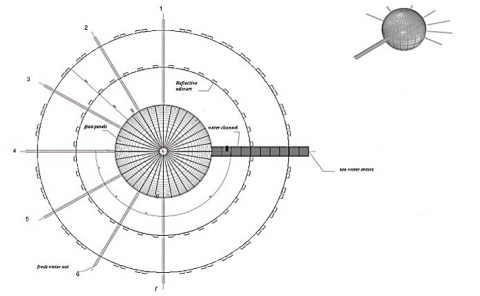
A schematic for the proposed solar dome design shown in Figure 3. The stimulating space is 0.85m2. The transparent surface of solar made of glass with a metal structure begins at an angle of 10° with horizontal surface and ends at 180°. The water level was 5cm, with concentrated mirrors surrounding the dome to focus the radiation and increase evaporation rate. Other dimensions are described in Figure 3. 2D geometric model, border terms and uneulogized networks are explained in Figure 4.
To solve the equations of continuity and momentum, the proper boundary conditions have been set for each of the boundary terms. The 12-hour CFD simulation timeframe necessary for solar dome modeling, which is a non-steady state process, is impracticable due to the enormous amount of time steps & computer time limits. The basin's solar energy absorption, as well as the water & glass temperature contained inside, were anticipated to remain constant during a one-hour time period. The glass, bottom, and bottom factor boundary conditions were used to produce constant temperature limitations. At 9:00 a.m. Until 8 p.m., the mean temperature was used as the boundary condition for each 1-hour time period. The bottom temperature was observed to be comparable to the glass temperature. The temperatures in the bottom and heat tanks were similar. The absorption factor & emission of the glass, water, & bottom all contribute to the sun's intensity. When constructing the fall against the glass, the simulations took adhesion forces into account. The side walls were originally intended to be adiabatic. For the liquid phase, the non-slip wall boundary condition was employed, but for the gas phase, the free-slip boundary condition was applied. The volume fractions of water and mixture were calculated to be 0.14 & 0.95, respectively, based on the system's beginning water level of 5cm. Evaporation resulted in a reduction in the water level. As a result, the water level is varied throughout the following procedures to calculate the pressure. The system pressure, in other words, is proportional to the hydrostatic pressure at the static water level.
Figure 3. Schematic for the proposed solar dome design
Figure 4. Geometry and mesh of the model
The ANSYS application was utilized to carry out the CFD analysis, and parallel runs were used to solve the equations [24]. According to the computer utilized for the CFD simulation, it took about 12 hours to compute each simulation needed to attain a quasi-steady state. The geometry of the build & mesh model was performed using ANSYS Workbench 18. An unstructured grid of circular surface type was used. Thus, to reduce the computational effort, simulations were performed with 48,279 knots. The goal of this research is to create a computational fluid dynamics model of the solar dome's evaporation and condensation processes. The water in the system evaporates due to solar energy. The temperature difference between the water vapor & the glass causes the vapor to condense on the surface of the glass. The drops slip and collect on the duct. To calculate the fresh water in the simulations, the quantity of water accumulating on the lower stream was taken as the water production rate.
The stationary area gradually becomes saturated with water vapor, and the rate of freshwater production rises until around 15:00 PM in the summer and autumn. Then, when solar radiation is reduced, the quantity of water created gradually declines. The droplets on the glass are little in comparison to its surface. The water volume fraction profiles matching to the system's side view are displayed in Figure 5. The liquid and gas phases are fully different from one another, as is their interface. The liquid phase is visible only on the glass, the bottom, and the geometry of the model. In the still state, the temperature of the gas phase in each phase is roughly constant.
Figure 5. Contour volume of water in a solar dome
The temperature profile of the combination is shown in Figure 6, Figure 7 depicts the gas velocity vector at the plane within the solar dome. Between the bottom and the glass, the gas phase follows circular route lines. The heated phase rises owing to the buoyant force and condenses on the glass. While Figure 8 shows the evaporation rate resulting from the process of concentrating the intensity of solar radiation inside the solar dome.
Figure 6. Temperature of the mixture inside the solar dome
Figure 7. Velocity vector of the mixture on a plane inside the solar dome
Figure 9 also illustrates that the months of April to October have the greatest average temperature of 85℃. In addition, the minimum temperature in June is 45℃. The storage compartment has an annual average temperature of 70℃, which is about 50°C higher than the ambient temperature. As a result, the water output of the solar dome varies substantially depending on the season.
Based on the program data, Figure 10 depicts the glass, heat tank, and water temps. As a boundary condition, the mean temperature was chosen. The bottom temperature was determined to be the same as the glass temperature. The temperatures in the bottom and heat tanks were the same.
Figure 8. Evaporation volume inside the solar dome
Figure 9. One-year projection of changes in storage area temperature for the reference solar dome, without heat removal
Figure 10. Temperature changes of different elements in the solar dome
Figure 11. Fresh water production rate
Figure 12. The water temps by the CFD simulation
Figure 13. The rate of heat transfer by evaporation
The results of conducting the simulation over a 12-hour period are shown in Figure 11. The commencement of the procedure at 8:30 AM exceeds the time when the water temperature rises in locations that are still warming owing to solar radiation, as shown in this diagram. The stationary region gradually becomes saturated with water vapor & the rate of freshwater production rises until around 14:00 PM. The amount of water created gradually decreases as solar radiation is reduced.
The water temperatures predicted by the CFD simulation are shown in Figure 12. It changes in a similar way to the explanations given in Figure 10.
The results of the CFD simulation using the mentioned model, as well as the hcw and hew of Dunkle's relationship from the data (CFD) were shown in Figure 13 and Figure 14. CFD predictions are clearly acceptable. The trend of differences in heat transfer coefficients is similar to the temperature change number; Because both hcw & hew are dependent on the temperature of the water and the glass.
Figure 14. Heat transfer coefficient by convection (hcw)
Desalination is a possible solution to water scarcity, given that 70% of humanity lives within 120 kilometers of an ocean, Desalination enhances the quality of water, alleviates water scarcity, and enhances people's quality of life & financial situation. Humans now rely significantly on fossil fuels for energy. Use of fossil fuels has led to significant ecological and environmental problems, including global warming. Furthermore, the limited quantity of fossil fuels is depleted by their indiscriminate use. As a result, demand must be controlled and new energy sources must be created. The cost of solar-powered desalination plants is compared in Table 1 [24-31]. The combination of solar energy with desalination technology has significant room for development; Expenditures associated with desalination contribute for 10%-20% of overall costs, while solar system costs account for 15%-70%. In summary, when economic and reliability concerns are considered, technical feasibility is often not a constraint.
Table 1. Solar-driven desalination system cost
|
Characteristics |
Irradiation |
Desalination Cost (%) |
Solar Systems Cost (%) |
Others Cost %)( |
Capacity |
|
HDH/OWCA [24] |
0-5000 W/m2 |
10.4 |
20.8 |
68.8 |
22 L/d |
|
HDH/OACW [25] |
300-550 W/m2 |
< 20 |
67 |
12.3 |
1.2 m3/d |
|
ORC-MED [26] |
503 W/m2 |
10 |
15 |
75 |
Pfreshwater=100 m3/d |
|
Wind-PV-diesel-battery-RO [27] |
1000 W/m2 |
16.7 |
50 |
33.3 |
Pfreshwater =24 m3/d Pcost =2.20 $/m3 |
|
Collector + MED with flash evaporation (for large system, 0.3 m3/d) [28] |
NA |
30 |
60 |
10 |
Pfreshwater =6 m3/d |
|
Collector + MED with flash evaporation (for large system, 0.3 m3/d) [28] |
NA |
26.7 |
66.7 |
6.6 |
Pfreshwater =0.3 m3/d |
|
Solar pond + MSF with PTC [29] |
NA |
43.1 |
50.2 |
6.7 |
Pfreshwater =1880 m3/d |
|
PV+RO with 2-stage ORC [30] |
NA |
61 |
39 |
NA |
NA |
|
Neom (Solar dome for large 50-80 m) [31] |
500 W/m2 |
NA |
NA |
NA |
Pfreshwater =30000 m3/h Pcost =0.34 $/m3 |
The solar dome's evaporation and condensation processes are reproduced in this paper. CFD was used to construct a 2-dimensional model. The model was created for a system that mixes water (air and water vapor). Within 12 hours of a one-hour period, experimental data were simulated. Solar light evaporated the water, and the model was able to calculate the quantity of water created. The Dunkle correlation was used to compute the convective & evaporative coefficients of heat transport. Coefficients of convective and evaporative heat transfer for simulation models 10 and 3 were determined. The projected findings demonstrate that computational fluid dynamics is an extremely strong tool for designing, assessing parameters, & deleting challenging components from stationary solar structures. In the still state, the temperature of the gas phase in each phase is roughly constant. The droplets on the glass are little in comparison to its surface. The stationary area gradually becomes saturated with water vapor, and the rate of freshwater production rises until around 15:00 PM in the summer. Circular route lines are followed by the gas phase between the bottom and the glass. Due to buoyant force, the heated phase rises and condenses on the glass. The experiment produces a stationary region that gradually becomes saturated with water vapor as it warms owing to solar radiation. Desalination enhances the quality of water, alleviates water scarcity, and enhances people's quality of life & financial situation. The combination of solar energy with desalination technology has significant room for development. When economic and reliability concerns are considered, technical feasibility is often not a constraint. The difference between this study and previous studies is the desalination model used so that the dome is available for water condensation from all sides and at an angle of 360 degrees. The study is the use of solar energy in water desalination with a new model in the form of a steel and glass dome. Most of the models in solar water desalination are in the form of a distiller with one or two sides or a flat box of limited size.
The authors would like to thanks Al-Mustaqbal University College, 51001 Hillah, Babylon, Iraq, for the assistance in completing this work.
[1] Allan, J.A. (1989). Water resource evaluation and development in libya-1969-1989. Libyan Studies, 20: 235-242. https://doi.org/10.1017/S0263718900006737
[2] Sa’ed, F. (1994). Water policies in the arab world up to the year 2000-analysis study.
[3] Xu, P., Cath, T.Y., Robertson, A.P., Reinhard, M., Leckie, J.O., Drewes, J.E. (2013). Critical review of desalination concentrate management, treatment and beneficial use. Environmental Engineering Science, 30(8): 502-514. https://doi.org/10.1089/ees.2012.0348
[4] Trivedi, H.K., Upadhyay, D.B., Rana, A.H. Seawater desalination processes.
[5] Harandi, H.B., Rahnama, M., Javaran, E.J., Asadi, A. (2017). Performance optimization of a multi stage flash desalination unit with thermal vapor compression using genetic algorithm. Applied Thermal Engineering, 123: 1106-1119. https://doi.org/10.1016/j.applthermaleng.2017.05.170
[6] Eveloy, V., Rodgers, P., Qiu, L. (2015). Hybrid gas turbine-organic rankine cycle for seawater desalination by reverse osmosis in a hydrocarbon production facility. Energy Conversion and Management, 106: 1134-1148. https://doi.org/10.1016/j.enconman.2015.10.019
[7] Jiang, S., Li, Y., Ladewig, B.P. (2017). A review of reverse osmosis membrane fouling and control strategies. Science of the Total Environment, 595: 567-583. https://doi.org/10.1016/j.scitotenv.2017.03.235
[8] Shemer, H., Semiat, R. (2017). Sustainable RO desalination–energy demand and environmental impact. Desalination, 424: 10-16. https://doi.org/10.1016/j.desal.2017.09.021
[9] Eltawil, M.A., Zhengming, Z., Yuan, L. (2009). A review of renewable energy technologies integrated with desalination systems. Renewable and Sustainable Energy Reviews, 13(9): 2245-2262. https://doi.org/10.1016/j.rser.2009.06.011
[10] Dunkle, R.V. (1961). Solar water distillation: The roof type still and a multiple effect diffusion still. In Proc. International Heat Transfer Conference, University of Colorado, USA, 1961, 5: 895.
[11] Agha, K.R. (2009). The thermal characteristics and economic analysis of a solar pond coupled low temperature multi stage desalination plant. Solar Energy, 83(4): 501-510. https://doi.org/10.1016/j.solener.2008.09.008
[12] Tleimat, M.C., Howe, E.D. (1989). The use of energy from salt-gradient solar ponds for reclamation of agricultural drainage water in California: Analysis and cost Prediction. Solar Energy, 42(4): 339-349. https://doi.org/10.1016/0038-092X(89)90037-6
[13] Tabor, H. (1975). Solar ponds as heat source for low-temperature multi-effect distillation plants. Desalination, 17(3): 289-302. https://doi.org/10.1016/S0011-9164(00)84062-X
[14] Nielsen, C.E. (1976). Experience with a prototype solar pond for space heating. Sharing the Sun: Solar Technology in the Seventies, 5(5): 169-182.
[15] Authority, W.G.W. (2014). Water and energy for life in libya (WELL). Libya: The European Commission, 295143.
[16] Cedare. (2014). Libya water sector M&E rapid assessment report. Monitoring and Evaluation for Water in North Africa (MEWINA) Project, Water Resources Management Program.
[17] Brika, B. (2018). Water resources and desalination in Libya: A review. In Proceedings of the 3EWaS International Conference on Insights on the Water-Energy-Food Nexus, Lefkada Island, Greece, 27-30 J.
[18] Delyannis, E. (2003). Historic background of desalination and renewable energies. Solar Energy, 75(5): 357-366. https://doi.org/10.1016/j.solener.2003.08.002
[19] Darwish, M.A., Abdulrahim, H.K., Hassan, A.S., Mabrouk, A.A. (2016). PV and CSP solar technologies & desalination: Economic analysis. Desalination and Water Treatment, 57(36): 16679-16702. https://doi.org/10.1080/19443994.2015.1084533
[20] Ali, M.T., Fath, H.E., Armstrong, P.R. (2011). A comprehensive techno-economical review of indirect solar desalination. Renewable and Sustainable Energy Reviews, 15(8): 4187-4199. https://doi.org/10.1016/j.rser.2011.05.012
[21] Soliman, A.M., Al-Falahi, A., Mohamed AEldean, S., Elmnifi, M. (2020). A new system design of using solar dish-hydro combined with reverse osmosis for sewage water treatment: Case study Al-Marj, Libya. Desalination and Water Treatment, 193: 189-211. https//doi.org/10.5004/dwt.2020.25782
[22] Tiwari, G.N. (2002). Solar energy: Fundamentals, design, modelling and applications. Alpha Science Int'l Ltd.
[23] Jassim, L., Elmnifi, M., Elbreki, A., Habeeb, L.J. (2022). Modeling and analysis of home heating system material performance with induction using solar energy. Materials Today: Proceedings, 61: 852-859. https://doi.org/10.1016/j.matpr.2021.09.302
[24] Hamed, M.H., Kabeel, A.E., Omara, Z.M., Sharshir, S.W. (2015). Mathematical and experimental investigation of a solar humidification-dehumidification desalination unit. Desalination, 358: 9-17. https://doi.org/10.1016/j.desal.2014.12.005
[25] Yuan, G., Wang, Z., Li, H., Li, X. (2011). Experimental study of a solar desalination system based on humidification-dehumidification process. Desalination, 277(1-3): 92-98. https://doi.org/10.1016/j.desal.2011.04.002
[26] Sharaf, M.A., Nafey, A.S., García-Rodríguez, L. (2011). Exergy and thermo-economic analyses of a combined solar organic cycle with multi effect distillation (MED) desalination process. Desalination, 272(1-3): 135-147. https://doi.org/10.1016/j.desal.2011.01.006
[27] Gökçek, M. (2018). Integration of hybrid power (wind-photovoltaic-diesel-battery) and seawater reverse osmosis systems for small-scale desalination applications. Desalination, 435: 210-220. https://doi.org/10.1016/j.desal.2017.07.006
[28] Jiang, J., Tian, H., Cui, M., Liu, L. (2009). Proof-of-concept study of an integrated solar desalination system. Renewable Energy, 34(12): 2798-2802. https://doi.org/10.1016/j.renene.2009.06.002
[29] Al-Othman, A., Tawalbeh, M., Assad, M.E.H., Alkayyali, T., Eisa, A. (2018). Novel multi-stage flash (MSF) desalination plant driven by parabolic trough collectors and a solar pond: A simulation study in UAE. Desalination, 443: 237-244. https://doi.org/10.1016/j.desal.2018.06.005
[30] Kosmadakis, G., Manolakos, D., Kyritsis, S., Papadakis, G. (2009). Economic assessment of a two-stage solar organic rankine cycle for reverse osmosis desalination. Renewable Energy, 34(6): 1579-1586. https://doi.org/10.1016/j.renene.2008.11.007
[31] Sustainably solving the water crisis, http://solarwaterplc.com, accessed on 10 May, 2023.