Modified Secant Method for Reduction in Number of Iterations

The present work aims to find improvement in the non-linear equation solutions that require many iterations. The secant method is one of the best, considering its faster convergence rate than the Regula Falsi and Bisection method. The formulation uses three successive points of the iteration instead of just two, and the order of convergence is 1.839 [1]. An improved Newton Raphson’s method has been developed, where a definite area integral is approximated as trapezoidal area in place of the rectangular area [2]. A zero-finding method is used to solve non-linear equations, which is most efficiently used with the traditional iterative method in which the order of convergence is improved [3]. The leap-frog Newton's method has been developed using Newton's method as an intermediate step. At a simple root, the order of convergence is cubic, and the computational efficiency is lower but still quite comparable to Newton's approach [4]. To approximate a locally unique solution of a non-linear equation in Banach spaces, the idea uses Lipschitz and center–Lipschitz instead of just Lipschitz conditions in the convergence analysis [5]. An improved Regula-Falsi method with an order of convergence of 3 combines the usual Regula-Falsi method and a Newton-like method to solve for f(x) = 0 [6]. A novel approach for solving non-linear equations that is similar to the Secant method. The convergence analysis reveals that the asymptotic order of convergence of this method is $(1+\sqrt{3})$ [7]. A modified secant method is analysed under the hypothesis of second-order derivatives (Lipschitz continuous) with an error analysis [8]. An improved Regula Falsi (IRF) method based on the classic Regula-Falsi (RF) method has been tested considering many numerical examples and the results confirm that the proposed method performs well compared to the traditional Regula-Falsi method [9]. Another novel class of spectral conjugate gradient algorithms studied to achieve high-order accuracy in predicting the second-order curvature [10]. To obtain similar convergence to Newton's approach without analyzing any derivatives, a generalization of the Secant method to semi-smooth equation is suggested [11]. The Newton-Raphson method makes it clear that the correction needed to obtain the right value of the root decreases as the derivative f^’(x) increases [12]. To increase the Secant method's applicability, changes have been made to the resolution of a linear system in each step required to use the secant approach for multiple matrix multiplications [13]. To solve a non-linear equation, modification has been done using the secant method, which involves the development of the inverse of the first-order divided differences of a function of several variables at two points [14]. Although the Newton-Raphson method converges quickly close to the root, its global characteristics are poor [15]. Several researchers tried to reduce the number of iterations, which reduces the computational cost of the Secant method. The present paper aims to find an improved method that is faster than the standard Secant method. According to the present study, some changes to the Secant method's standard conditions are required. These conditions are as follows:

Condition 1: - Either $f\left(x_a\right) * f\left(x_b\right)$  or $f\left(x_a\right) * f\left(x_b\right)>0$

where, x_a and x_b are two initial guesses, and f(x_a) and f(x_b) are function value. It demonstrates that the signs of f(x_a) and f(x_b) can be opposite or identical. The Modified Secant method also satisfied the requirement mentioned above, which is true.

Condition 2: - After making two initial estimations, x_a and x_b, the first root value can be calculated using the standard Secant formula. If the value obtained is x₁, then the equation has a root only if f(x₁)=0; otherwise, f(x₁)>0 or f(x₁)<0. Now, the formula for the following iterations includes two values, one of which is the new iteration value, i.e., x₁, and the other one is immediately before it, i.e., x_b but not x_a.

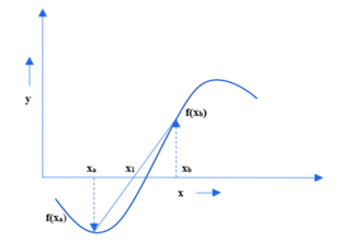
This Modified Secant approach no longer allows condition- 2. The entire fundamental is based on condition 2. The Modified Secant approach has been developed in this paper, which will also show the transformation of the standard Secant method into the Modified Secant method. The reader must have an understanding of triangular properties. Consider Figure 1, where x_a and x_b are the two roots. Draw a chord that joins two points, f(x_a) and f(x_b), due to this chord, we now have two triangles i.e., $\Delta\left(f\left(x_a\right), x_1, x_a\right)$  and $\Delta\left(f\left(x_b\right), x_1, x_b\right)$ , we can use similar triangular properties to solve the standard Secant formula. As we know, triangular properties are:

• The two triangles must be of the same shape, and their size may vary,
• Each pair of corresponding angles are equal,
• Corresponding sides are in the same proportion.

1.png

Figure 1. Function curve with two initial guesses i.e., x_a and x_b

Figure 1 shows the two function values, f(x_a) and f(x_b)are of opposing signs.

The two most recent root approximations are used to find the next approximation in the standard Secant technique [16].

The Modified Secant method applied immediately after the first iteration, and the starting formulation remains the same for Regula Falsi, the Secant method, and the Modified Secant method. Let two initial guesses be, $x_a$ and $x_b$(the function values of both negative, and positive, or one negative and one positive, have no effect on the initial formula) [17]. By employing a similar triangular property. The first iteration formula is as follows: Refer to Figure 1.

2.png

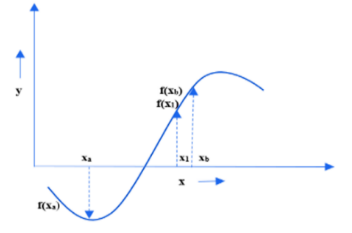
Figure 2. Function curve with three roots, i.e., x_a, x_b and x₁ for finding x₂

$\begin{gathered}\frac{\left(x_1-x_a\right)}{\left(-f\left(x_a\right)\right)}=\frac{\left(x_b-x_1\right)}{f\left(x_b\right)} \\ f\left(x_b\right) * x_1-f\left(x_b\right) * x_a=\left(-f\left(x_a\right) * x_b\right)+f\left(x_a\right) * x_1 \\ f\left(x_b\right) * x_1-f\left(x_a\right) * x_1=\left(-f\left(x_a\right) * x_b+f\left(x_b\right) * x_a\right. \\ \left(f\left(x_b\right)-f\left(x_a\right)\right) * x_1=f\left(x_b\right) * x_a-f\left(x_a\right) * x_b \\ x_1=\frac{\left(x_a * f\left(x_b\right)-x_b * f\left(x_a\right)\right)}{\left(f\left(x_b\right)-f\left(x_a\right)\right)}\end{gathered}$    (2)

For the second iteration, use the conditions (A and B): Since the modified approach will compute after the first iteration, it's critical to illustrate the second iteration formula. Refer to Figure 2.

If $a b s\left(f\left(x_a\right)\right)-a b s\left(f\left(x_1\right)\right)<a b s\left(f\left(x_b\right)\right)-a b s\left(f\left(x_1\right)\right)$ use x_a with x₁ for new iteration (A).

$\begin{gathered}\frac{\left(x_2-x_a\right)}{\left(-f\left(x_a\right)\right)}=\frac{\left(x_1-x_2\right)}{f\left(x_1\right)} \\ f\left(x_1\right) * x_2-f\left(x_1\right) * x_a=-f\left(x_a\right) * x_1+f\left(x_a\right) * x_1 \\ f\left(x_1\right) * x_2-f\left(x_a\right) * x_2=-x_1 * f\left(x_a\right)+f\left(x_1\right) * x_a \\ \left(f\left(x_1\right)-f\left(x_a\right)\right) * x_2=f\left(x_1\right) * x_a-x_1 * f\left(x_a\right) \\ x_2=\frac{\left(x_a * f\left(x_1\right)-x_1 * f\left(x_a\right)\right)}{\left(f\left(x_1\right)-f\left(x_a\right)\right)}\end{gathered}$    (3)

If $a b s\left(f\left(x_b\right)\right)-a b s\left(f\left(x_1\right)\right)<a b s\left(f\left(x_a\right)\right)-a b s\left(f\left(x_1\right)\right)$use x_b with x₁ for new iteration (B).

$\begin{gathered}\frac{\left(x_b-x_2\right)}{f\left(x_b\right)}=\frac{\left(x_1-x_2\right)}{f\left(x_1\right)} \\ x_b * f\left(x_1\right)-x_2 * f\left(x_1\right)=f\left(x_b\right) * x_1-f\left(x_b\right) * x_2 \\ x_b * f\left(x_1\right)-f\left(x_b\right) * x_1=x_2 * f\left(x_1\right)-f\left(x_b\right) * x_2 \\ x_b * f\left(x_1\right)-f\left(x_b\right) * x_1=\left(f\left(x_1\right)-f\left(x_b\right)\right) * x_2 \\ x_2=\frac{\left(x_b * f\left(x_1\right)-x_1 * f\left(x_b\right)\right)}{\left(f\left(x_1\right)-f\left(x_b\right)\right)}\end{gathered}$    (4)

The standard Secant technique requires only one formula to solve for the second iteration; however, the modified Secant method employs two conditions (A and B) on the second iteration.

3.1 Proof of the modified secant method

The Regula Falsi, Secant technique and Modified Secant method require two initial guesses to solve non-linear equations. The modified procedure starts after the first iteration since it requires three function values to meet conditions (A and B).

The Secant method has the disadvantage that it cannot approximate the root value more accurately with each iteration, which makes the function value close to zero. By presenting conditions (A and B), the problem has been eliminated. The physical relevance of these two requirements has been reduced to a bare minimum computational cost. Afterwards, one must consider the second condition (mentioned in the introduction). For the second approximation root, the Secant approach is employed x_b with x₁, but not x_a with x₁. The Secant approach does not provide any information about x_a with x₁. Therefore, these two conditions (A and B) are introduced to clarify this. These two conditions connect new approximate roots and older roots to meet the situation best. Consider condition (A) (mentioned in the introduction part); in this case, the left-hand side difference is less than the right-hand side difference. This distinction is significant because it reveals how these roots are best selected after each iteration. These two conditions (A and B) can be used to achieve this.

A straightforward illustration Consider the initial predictions, x_a and x_b. Let's use the values f(x_a))= 2, f(x_b)=3, and f(x₁)=1.8, The modified secant technique will then satisfy conditions (A and B) by using the value of f(x_a), f(x_b) and f(x₁) for the next iteration, i.e., x₂, which will aid in finding functions near zero. The Modified Secant method stops performing once the differences between the left-hand and right-hand sides in either of the conditions (A or B) are less than the error, which depends on the type of problem setting, whether the condition is satisfied or not, and works as a stopping criterion.

Conditions (A and B) follow the Secant method requirement to show the Modified Secant Method.

If $\operatorname{abs}\left(f\left(x_a\right)\right)-a b s\left(f\left(x_1\right)\right)<a b s\left(f\left(x_b\right)\right)-a b s\left(f\left(x_1\right)\right)$ use x_a with x₁ for 2^nd iteration. (A)

If $a b s\left(f\left(x_b\right)\right)-a b s\left(f\left(x_1\right)\right)<a b s\left(f\left(x_a\right)\right)-\operatorname{abs}\left(f\left(x_1\right)\right)$ use x_b with x₁ for 2^nd iteration. (B)

x_a = 1^st initial guess

x_b = 2^nd initial guess

x₁ = 1^st approximate root after the first iteration using formula 2, given above.

f(x_a) = Function value of 1^st initial guess

f(x_b)Function value of 2^nd initial guess

f(x₁) Function value of 1^st approximate root

According to the secant or chord method: -

1. $\operatorname{abs}\left(f\left(x_1\right)\right)$ is always lower than $\operatorname{abs}\left(f\left(x_a\right)\right)$ and $\operatorname{abs}\left(f\left(x_b\right)\right)$
2. $f\left(x_a\right) * f\left(x_b\right)<0$ or $f\left(x_a\right) * f\left(x_b\right)>0$ where, $f\left(x_a\right) \neq f\left(x_b\right)$

The Modified Secant method meets the standard Secant method's criteria and adds these two conditions (A and B). This approach is now more accurate than the previous standard Secant method, and the number of iterations has been reduced. Because there are three roots available, the information acquired from these two conditions (A and B) means that a choice can be made between the two older approximate roots and the new approximate root in order to determine the subsequent approximate root.

3.2 Procedure for the modified secant method

The following are the steps to be considered in the proposed modified Secant method.

Step 1: - Consider two initial guesses, let's say, x_-1 and x₀

Step 2: - Put x_-1, x₀, f(x_-1), f(x₀) in general, the formula is given below.

$x_{i+1}=\frac{\left(x_{i-1}\quad * f\left(x_i\right)-x_i * f\left(x_{i-1}\quad\right)\right)}{\left(f\left(x_i\right)-f\left(x_{i-1}\quad\right)\right.}$    (5)

For the 1^st iteration, i = 0.

Step 3: - Use Conditions (A and B) for the 2^nd iteration.

If $a b s\left(f\left(x_a\right)\right)-a b s\left(f\left(x_1\right)\right)<a b s\left(f\left(x_b\right)\right)-a b s\left(f\left(x_1\right)\right)$ use x_a with x₁ for 2^nd iteration (A):

here, $x_a=x_{-1}$ and $x_b=x_0$:

$x_2=\frac{\left(x_{-1} \quad* f\left(x_1\right)-x_1 * f\left(x_{-1}\quad\right)\right)}{\left(f\left(x_1\right)-f\left(x_{-1}\quad\right)\right)}$    (6)

If $a b s\left(f\left(x_b\right)\right)-a b s\left(f\left(x_1\right)\right)<a b s\left(f\left(x_a\right)\right)-a b s\left(f\left(x_1\right)\right)$ use x_b with x_a for 2^nd iteration (B).

$x_2=\frac{\left(x_b * f\left(x_1\right)-x_1 * f\left(x_b\right)\right)}{f\left(x_1\right)-f\left(x_b\right)}$    (7)

Step 4: - Stop executing once the left-hand and right-hand side differences in any of the conditions are less than the error. If the condition is satisfied, use conditions (A and B) as a stopping criterion.

Step 5: - Repeat step 3 for the 3^rd iteration. 

Either condition (A) or condition (B) is met, use the following formula pattern:

$x_{\text {next }}=\frac{\left(x_{\text {old }} \,\,* f\left(x_{\text {new }}\,\,\right)-x_{\text {new }} \,\,* f\left(x_{o l d}\,\,\right)\right)}{\left(f\left(x_{n e w}\,\,\right)-f\left(x_{o l d}\,\,\right)\right)}$   (8)

where, $x_{n e x t}=x_{i+1}, i=2$

$x_{\text {old }}=x_{i-1}, i=2$ and $i=1$

$x_{n e w}=x_i, i=2$

Two values of $x_{\text {old }}$at different (i) represent two old approximate roots as per applicability of conditions (A and B) while x_new represents a new approximate root.

For subsequent iterations i=3,4,5………. n, n = Real number.

3.3 Flow chart for steps involved in the proposed modified method

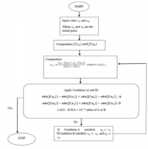
Figure 3 shows the flow chart of modified secant method.

tu_pian_1.png

Figure 3. Flow chart for modified secant method

5.1 Comparison and validation 1

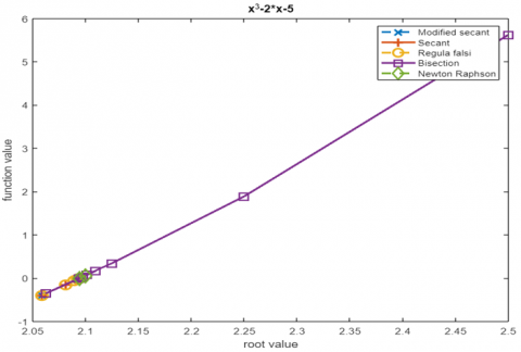
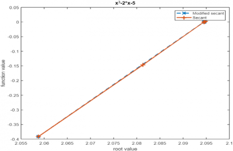
Consider f(x)= x³-2^*x-5    

1^st initial guess = 2, 2^nd initial guess = 3

Final root = 2.0946

Modified Secant Method = 4 Iteration

Secant Method = 5 Iteration

Regula Falsi Method = 10 Iteration

Bisection Method = 15 Iteration

Newton Raphson Method = 2 Iteration

Values obtained using different root finding methods are tabulated in Table 1 and 2.

Table 1. Comparison of various methods for a lower number of iterations

Modified Secant Method	Secant Method	Regula Falsi Method	Bisection Method	Newton Raphson Method
X1=2.0588	X1=2.0588	X1=2.05882	X1=2.5000	X1=2.1000
X2=2.0966	X2=2.0813	X2=2.08126	X2=2.2500	X2=2.0946
X3=2.0945	X3=2.0948	X3=2.08964	X3=2.1250
X4=2.0946	X4=2.0945	X4=2.09274	X4=2.0625
	X5=2.0946	X5=2.09388	X5=2.0938
		X6=2.09431	X6=2.1094
		X7=2.09466	X7=2.1016
		X8=2.09452	X8=2.0977
		X9=2.09454	X9=2.0957
		X10=2.09455	X10=2.0947
			X11=2.0942
			X12=2.0945
			X13=2.0946
			X14=2.0945
			X15=2.0946

a.png

(a) Function vs Root value

b.png

(b) Function vs Root value

c.png

(c) Function vs Root value

d.png

(d) Function vs Root value

Figure 4. (a) Function vs Root value; (b) Function vs Root value; (c) Function vs Root value; (d) Function vs Root value

The figures above shows the comparison of root finding method.

Figure 4 (a) shows comparisons between the Modified Secant Method and Standard Secant, Regula Falsi, Newton Raphson and Bisection method for a lower number of iterations.

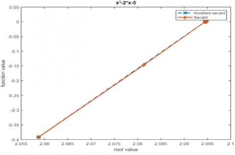
Figure 4 (b) shows comparisons between the Modified Secant method and Standard Secant, Regula Falsi and Newton Raphson method for the lower number of iterations.

Figure 4 (c) shows comparisons between the Modified Secant method and Standard Secant and Regula Falsi method for the lower number of iterations.

Figure 4 (d) shows comparisons between Modified Secant and Standard Secant methods for lower number of iterations.

From the present study, it is concluded that the Modified secant method has only four iterations, which can be easily found in Figures 4 (a), (b), (c) and (d) when compared with standard secant, Regula Falsi, and the Bisection method. In Figure 4 (a), compared to Newton Raphson's method, the Modified Secant method requires fewer iterations, but not as much.

5.2 Comparison and validation 2

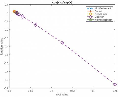
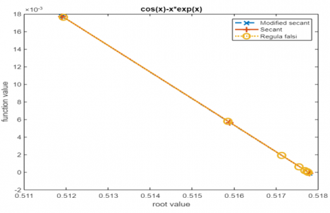
Consider f(x)= cos(x)-x*exp(x)

1^st initial guess = 0.5, 2^nd initial guess = 1

Final root = 0.5178

Modified Secant method = 2 Iteration

Secant method = 3 Iteration

Regula Falsi method = 8 Iteration

Bisection method = 13 Iteration

Newton Raphson method = 2 Iteration

Table 2. Comparison of various methods for a lower number of iterations

The figures below shows the comparison of root finding method.

Figure 4 (e) shows the function value against the root value for the Modified Secant Method, Standard Secant, Regula Falsi, Newton Raphson and Bisection method for the lower number of iterations.

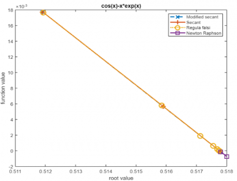
Figure 4 (f) shows function value against root value for Modified Secant method, Standard Secant, Regula Falsi and Newton Raphson method for a lower number of iterations

Figure 4 (g) shows function value against root value for Modified Secant method with Standard Secant and Regula Falsi, the method for a lower number of iterations.

Figure 4 (h) shows function value against root value for the Modified Secant method and Standard Secant method for a lower number of iterations.

It can be seen from Figures below that the modified secant method has two iterations, whereas the standard secant method has three iterations. The same can be seen in Figures 4 (e), 4 (f) and 4 (g). The present study concludes that modified secant method conditions (A and B) work on finding those roots which give solution faster than the standard Secant method.

e.png

(e) Function vs Root value

f.png

(f) Function vs Root value

g.png

(g) Function vs Root value

h.png

(h) Function vs Root value

Figure 4. (e) Function vs Root value; (f) Function vs Root value; (g) Function vs Root value; (h) Function vs Root value