Arief Goeritno*![]() | Muhammad Nanang Prayudyanto
| Muhammad Nanang Prayudyanto![]() | Puspa Eosina
| Puspa Eosina![]() | Tika Hafzara Siregar
| Tika Hafzara Siregar![]() | Roy Waluyo
| Roy Waluyo![]()
© 2023 IIETA. This article is published by IIETA and is licensed under the CC BY 4.0 license (http://creativecommons.org/licenses/by/4.0/).
OPEN ACCESS
The ideas of the studies in this article are back-grounded by the work diligently and carefully to relate the influence of two independent variables, e.g., distance and time on one dependent variable, i.e., temperature changes which are solved by a partial differential equation. In this article, we explain the particular features of a naturally physical system that it seeks to understand. The diagnosis of the temperature changes in a metal rod to consider a conduction phenomenon can be covered by all-natural physical phenomena through conduction. By making the mathematical equations based on partial differential equations (PDEs), it is shown that the temperature change is influenced by distance and time. The objectives of this study are (i) to make a prototype of the problem based on the one-dimensional heat conduction equation, (ii) to process the solution of the mathematical equation based on the parabolic partial differential equation (PDE) using the separation of variables, and (iii) to display the phenomena of the temperature changes as a function of the length in the copper bar and the time. Achieving the research objectives takes several stages in the research methods which include (a) making the prototype of the problem, (b) processing the solution of a mathematical equation, and (c) displaying the temperature changes phenomenon in the form of a curve. The results are (i) a mass balance is developed for a finite segment ![]() along the tank’s longitudinal axis in order to derive a differential equation, (ii) the final complete solution in the form of a Fourier sine series, and (iii) a three-dimensional curve as an indication of the existence of the phenomenon of temperature changes. In general, it can be concluded that the making of a mathematical model based on partial differential equations with the method of separating variables as an analytical solution can be used to diagnose the phenomenon of temperature changes as a function of distance and time.
along the tank’s longitudinal axis in order to derive a differential equation, (ii) the final complete solution in the form of a Fourier sine series, and (iii) a three-dimensional curve as an indication of the existence of the phenomenon of temperature changes. In general, it can be concluded that the making of a mathematical model based on partial differential equations with the method of separating variables as an analytical solution can be used to diagnose the phenomenon of temperature changes as a function of distance and time.
PDE-base mathematical models, diagnose the temperature changes phenomena, single rectangular plate-fin
Physics is a science that studies the order of the universe and as much as possible uses that order for two important things [1, 2], namely (i) discovering other regularities in the universe that have not been discovered and (ii) exploiting the order that has been found to be useful for human life [3]. Physics complements the existence of the trinity of the original hard sciences, in addition to the other two, i.e., chemistry and biology [4, 5]. In physical phenomena, the term “mathematical model” or to be known as a “model” is going to refer to a set of consistent equations intended to explain the particular features or behavior of a naturally physical system that it seeks to understand [6, 7]. The dynamics of a physical system are often described by differential equations, therefore the performance of physical systems is obtained by utilizing the physical laws of mechanical, electrical, fluid, and thermodynamic systems. The formation of mathematical models of physical phenomena of science and engineering models based on partial differential equations can be implemented through the elimination of constants or functions [8]. A diagnosis is an act of identifying a problem by examining something, therefore whatever that problem may be or the identification or naming of it is the diagnosis. The diagnosis of the temperature changes to cover all-natural physical phenomena can be through conduction, convection, or radiation [9, 10]. For the case of temperature change in a metal rod to consider a conduction phenomenon.
Mathematical modeling represents a very effective and powerful instrument to solve complex problems in various sciences, engineering, and technologies for comprehending the world of academic perspectives [11]. The models of equations in mathematics with the widespread use of differential equations, more specifically partial differential equations (abbreviated in the following as PDE in singular usage and PDEs in plural usage) can be found in various fields of natural, life, and social sciences [12]. A number of prominent phenomena in the natural science and particularly in physics can be approximated by PDEs [13-19] in (i) the change of the distance on the dimensions of space (the axes of x, y, and z) and (ii) in the change of the time (t) simultaneously, such as the distribution of heat (H) or temperature (T) in all directions of the axes of x, y, and z [20]. The PDEs describe the change of a system rather than its state over space and time, such changes in more than one independent variable, i.e., the variables of t, x, y, and z. A change in a system in space and time can be described by PDEs [21].
For assuming, knowing the solution at the time and all directions can be used as a PDE and describes a system to analytical and/or numerically estimate the solution after a very small change in time and all directions [21]. The law for energy conservation in solids and fluids can be described as a PDE for expressing the changes in temperature (T) in the space, therefore in this case, the temperature (T) is called the dependent variable [22]. It is can be selected a position in space and time for getting a unique value for the temperature by solving the PDEs, therefore-called the temperature depends on x, y, z, and t. However, a value of the temperature taken from the solution by PDEs, but does not automatically give us the position in time and space. In this sense, the parameters of x, y, z, and t are independent of temperature [20, 23].
The general form of a single rectangular fin is guided by the description in the book entitled "Transport Phenomena" written by Bird et al., in 1962 [23] and in this case specifically a single rectangular plate-fin made of copper metal that refers to the results of dissemination that written by Goeritno [24, 25]. A single rectangular plate-fin with a lengthiness (L) much greater than a thickness (B) [23-25] is shown in Figure 1.
Figure 1. A single rectangular plate-fin with a lengthiness (L) much greater than a thickness (B)
A reasonably good description of the system may be obtained by approximating the realistic situation and just on a model [23-25]. The comparison between the true physical situation and the simplified model [23, 24] is shown in Table 1.
A thermal energy balance on a segment $\Delta z$ of the bar gives the Eq. (1) [23, 24].
$\left.q_z\right|_z \cdot 2 BW -\left.q_z\right|_{z+\Delta z} \cdot 2 BW -h(2 W \cdot \Delta z)\left(T-T_a\right)=0$ (1)
Divided by $2 B W \cdot \Delta z$ and taking the limit $\Delta z$ approaches zero gives as the Eq. (2) $[23,24]$.
$-\frac{d}{d z} q_z=\frac{h_{m e t .}}{ B }\left(T-T_a\right)$ (2)
Assuming PDEs can be used to describe the laws of physics, then the solving of PDEs in a mathematical model makes it possible to predict the outcome of an experiment and helps engineers and scientists understand the phenomena that are described by that mathematical model. By making mathematical equations based on partial differential equations [24], it is shown that temperature change is influenced by time and distance (direction in space) [25]. In general, changes in the value of parameters as a function of the distance and the time through the simulation can be implemented [24]. Once validated, the solution of the PDEs, in combination with methods for varying model parameters, can also be used to optimize the design of a device or the phenomena of processes [13-19].
Making the mathematical models for implementing a single rectangular plate-fin as a passive heat exchanger for a fluid cooling process is an application of PDEs to diagnose the temperature parameter value per unit of distance and time [24, 25]. Several descriptions have become the basis [12-16], therefore the objectives of this study are (i) to make a prototype of the problem based on the one-dimensional (1-dim) heat conduction equation [26-30], (ii) to process the solution of the mathematical equation based on parabolic PDE using the separation of variables [13-19], and (iii) to display the phenomena of the temperature changes as a function of the length in the copper bar and the time [24, 25]. After achieving the objectives in this study, it is hoped that the purposes will be obtained through the procedures, namely (a) for making the 1-dim-based the prototype of problem that used the heat conduction equation for a finite segment in the z-axis, (b) for processing the solution based on the parabolic PDE in the form of a Fourier sine series, and (c) for displaying the temperature changes phenomena in the form of curves that used a three-dimensional curve as an indication of the existence of the phenomenon of temperature changes through the calculation process on the conditions of these physical phenomena [31]. The rest of this article is organized as follows, i.e., chapter 2 presents our proposed materials and methods of the studies, chapter 3 presents the results and discussion, and chapter 4 presents the conclusion.
Table 1. The comparison between true physical situation and the simplified model
|
True Physical Situation |
No. |
The Simplified Model |
|
Temperature (T) is a function of the z-axis, which is more important, although it is actually a function both axes, i.e., axes of x and z. |
#1 |
T is a function of the z-axis alone. |
|
A small quantity of heat is lost from the fin at the end (area of 2BW) and the edges (area of 2BL+2BL). |
#2 |
No heat is lost from the end or the edges. |
|
The coefficient of heat transfer is a function of position. |
#3 |
The heat flux at the surface is given by q=h(T-Ta ), which h is constant, and T=T(z). |
2.1 Materials of the study
As is known, the general solution to the ordinary differential equation (ODE) involves an arbitrary constant, while the general solution to the PDE involves an arbitrary function. The PDE is an equation in which there are two terms of partial differential, i.e., (i) which in mathematics is defined as a relationship that relates to an unknown function, and (ii) which is a function of several independent variables, with their derivatives through variables that meant [13-19]. The PDE is a differential equation in which the unknown function is a function of many independent variables, and the equation also involves partial derivatives [13-19, 12]. The PDE is used to formulate and solve problems involving unknown functions [13-19] which are formed by several variables, such as sound and heat propagation, electrostatics, electrodynamics, fluid flow, elasticity, or more generally all kinds of processes distributed in space, or distributed in space, i.e., one of the directions axes of x, y, or z and the time (t). The order of the equations is defined as in ordinary differential equations, but further classification into elliptic, parabolic, and hyperbolic, especially for second-order linear differential equations is very important [32]. Some PDEs cannot fall into these categories and are called mixed types [12].
The general linear PDEs of the second order in two independent variables are the form as Eq. (3) [33].
$\begin{gathered}A \frac{\partial^2}{\partial y^2} u(y, z)+B \frac{\partial^2}{\partial z \partial y} u(y, z)+C \frac{\partial^2}{\partial z^2} u(y, z) \\ +D\left(y, z, u, \frac{\partial}{\partial y} u, \frac{\partial}{\partial z} u\right)=0\end{gathered}$ (3)
where: A, B, and C are functions of y, z, and u.
The exact transformation to Eq. (3) is the same as transforming an equation of the form as Eq. (4) [33].
$A x^2+B x y+C y^2=0$ (4)
By a rotation of axes regarding the sign of B2-4AC which is called the value of discriminant, therefore the conversion into the standard forms of an elliptic, parabolic, or hyperbolic. Following the nomenclature of the geometrical configuration, if B2-4AC<0 the PDE is to be elliptic, if B2-4AC=0 is the PDE of parabolic type, and if B2-4AC>0 the PDE is called hyperbolic [18, 19, 33]. Each category describes through the different phenomena and mathematical properties that correspond to those phenomena [13-19].
A solution to the differential equation may depend on the time variable t, i.e., when the form of the function at t=0 is known as the initial condition for the differential equation. Likewise, it can be given the values of the functions in the boundary region as boundary conditions [34]. These two conditions can be written as a function with initial and boundary conditions and can be written as (i) ψ(0,t)=0, when t=0, and (ii) ψ(L,t)=1, when t>0. The completion of a PDE cannot be separated from someone's ability to solve an ODE, because the completion of a PDE can be brought into the form of an ODE in a certain way, for example by using a technique or method of variable separation [13-19]. Boundary conditions are certain conditions involved in the partial differential equation, therefore a solution to the partial differential equation can be searched. There are three possible boundary conditions, namely finite intervals, semi-finite intervals, and infinite intervals. For a finite interval, the value of the interval is 0<x<L, therefore it has two boundary conditions, namely at the beginning of x=0 and when x=L. For half-infinite intervals, the value of the interval is 0<x<∞ and is usually written x>0, therefore only the initial conditions are at x>0. For an infinite interval, the value of the interval is -∞<x<∞, therefore there is no boundary condition [13-19].
The form of the boundary condition equation is given by Eq. (5) [18, 19, 33].
$\left(\alpha U+\beta \frac{\partial}{\partial n} U\right)=f(x)$ (5)
where, α and β are constants and $\frac{\partial}{\partial n} U$ defined as shown in Eq. (6) [18].
$\operatorname{grad} . u \cdot n=\left(\frac{\partial}{\partial x_1} U, \cdots, \frac{\partial}{\partial x_n} U\right) \cdot n$ (6)
There are three possible types of boundary conditions for a second-order differential equation [35, 36], namely:
#a) Eq. (5) is called the Dirichlet’s condition, if α≠0 and β=0;
#b) Eq. (5) is called the von Neumann’s condition, if α=0 and β≠0; and
#c) Eq. (5) is called Robin’s condition or also called the mixed condition if α≠0 and β≠0.
Referring to Table 1 that T is a function of the z-axis alone, then the simplification of Eq. (5) is obtained the Eq. (7) [26-30].
$C \frac{\partial^2}{\partial z^2} T(z)+D\left(z, T, \frac{\partial}{\partial z} T\right)=0$ (7)
Eq. (7) is called the one-dimensional (1-dim, 1D) of PDE [26-30].
2.2 Methods of the study
Based on the previous research obtained the results [24, 25], namely (i) the change in temperature value on a copper bar in the form of a single rectangular plate-fin as a function of the length (as a function of the distance) and (ii) the change in temperature value on fluid as a function of the time. The results from the previous research are shown in Eqns. (8) and (9) [24].
$-\frac{d^2}{d z^2} T_{c u}=\frac{h_{c u}}{k_{c u} \cdot B}\left(T_{c u}-T_f\right)$ (8)
$\frac{d}{d t} T_f=-\frac{h_{c u} \cdot{ }^{“A”}{ }_{c u}}{m_f \cdot C_{p_f}} \cdot\left(T_{c u}-T_f\right)+\frac{U_w \cdot “A"{ }_w}{m_f \cdot C_{p_f}} \cdot\left(T_f-T_w\right)$ (9)
Referring to the Eq. (8), in that case of using copper material for the simulation process, then Tcu=T, hcu=hmet., and kcu=kmet., therefore the Eq. (8) transformed into the Eq. (10) [24].
$-\frac{d^2}{d z^2} T=\frac{h_{m e t .}}{k_{m e t .} \cdot \mathrm{B}}\left(T-T_f\right)$ (10)
Eq. (10) is used the plate-fin form in fluid, therefore for implementation in the air, then the Eq. (10) changes to Eq. (11) [24].
$-\frac{d^2}{d z^2} T=\frac{h_{m e t .}}{k_{\text {met. }} \cdot \mathrm{B}}\left(T-T_a\right)$ (11)
In Eq. (11) there is an insertion of Fourier's Law ($\left(q_z=-k \frac{d}{d z} T\right)$) [23, 24] in which the constant kmet. is k (coefficient of thermal conductivity of the metal), therefore Eq. (11) is changed like Eq. (2).
Diagnosing the changes in the value of parameters as a function of the distance or the time can be implemented by making mathematical equations based on the PDE [12-16]. Achieving the research objectives takes a number of stages in the research methods which include (a) making the prototype of the problem, (b) processing the solution of a mathematical equation, and (c) displaying the temperature changes phenomena in the form of the curve. Formatting the PDE can be implemented by eliminating the constant and function. In general, this method is done by eliminating the constants contained in a multi-variable function. Based on Eqns. (8) and (9), a PDE is made to obtain a one-dimensional (1-dim) heat conduction equation or known as the advection-diffusion equation as shown in Eq. (12) [26-30].
$\frac{\partial}{\partial t} T=-\frac{\partial^2}{\partial z^2} T$ (12)
The heat equation is a PDE describing the distribution of heat over time. In one spatial dimension as the temperature obeys the relation through a number of steps of completion according to the research objectives. A number of methods that can be used, especially for analytical solutions to PDEs include (i) separation of variables, (ii) method of characteristics, (iii) integral transform, (iv) change of variables, (v) fundamental solution, (vi) superposition principle, (vii) methods for non-linear equations, (viii) lie group method, and (ix) semi-analytical methods [12-16]. The further steps for solving a 1-dim heat conduction equation are when is used an analytical method [26-30]. Firstly, make the prototype of the problem based on the 1-dim heat conduction equation. Secondly, soluting the PDE when is used the method of separating variables. Thirdly as a final, giving the notation and displaying the curve.
3.1 Prototyping the problem
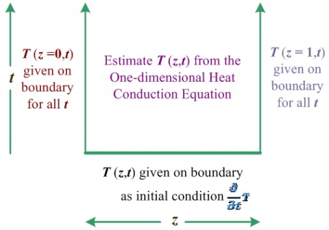
According to Eq. (12) is obtained A=-1, B=0, C=0, therefore by referring to Eq. (4), it is obtained the value of discriminant, i.e., B2-4AC=0 and the PDE is to be parabolic. Making the prototype of the problem based on the 1-dim heat conduction equation is the first stage to solve a problematic in the physic based on the PDE. Forming the PDE as Eq. (12) is typical example of one-dimensional heat conduction equation therefore the solution is done with a depiction or illustration. A depiction to explain the 1-dim heat conduction equation is shown in Figure 2.
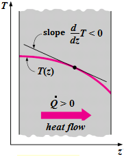
Based on Figure 2, it can be explained that all changes are propagated forward in time, i.e., nothing goes backward in time. The changes are propagated across space at decreasing amplitude. Considering the Figure 2, then a drawing is made for the phenomena of heat conduction. A depiction to explain further the one-dimensional heat conduction equation is shown in Figure 3.
Figure 2. A depiction to explain the 1-dim heat conduction equation
Figure 3. A depiction to explain further the one-dimensional heat conduction equation
Based on Figure 3, it can be explained that an elongated reactor with a single entry and exit point and a uniform cross-section of area “A”. A mass balance is developed for a finite segment.
$\Delta z$ along the tank’s longitudinal axis in order to derive a differential equation for “concentration of the temperature”, $T=A \cdot \Delta z$.
The one-dimensional heat conduction can be illustrated in the form of a diagram. An illustration of the one-dimensional heat conduction is shown in Figure 4.
Figure 4. An illustration of the one-dimensional heat conduction
Based on Figure 4, it can be explained that a diagram has been shown by Cengel's explanation in the reference of 26th.
The phenomenon of one-dimensional heat conduction is described as the simplest state of heat flow, so that heat flows in one face of the object and exits in the opposite face. The one-dimensional heat conduction equation is first used for solutions to homogeneous conditions, then the solution is substituted into one-dimensional non-homogeneous heat conduction. To solve one-dimensional non-homogeneous heat conduction by using Green's function with the result expressed in double integrals, while using the method of separating the variables, the result is expressed in a single integral.
3.2 Processing the solution of the mathematical equation
After obtaining the prototype of the problem based on the one-dimensional heat conduction equation, then further processing is carried out in the form of proceeding to determine the solutions using one of a number of the methods of analytical, i.e., it describes the solution process using the separation of variables. The equation for the energy balance in the heat conduction process is shown in Eq. (13) [18, 19, 33].
$\begin{gathered}V \frac{\Delta}{\Delta t} T=Q \cdot T(z)-Q\left[T(z)+\frac{\partial}{\partial z} T(z) \cdot \Delta z\right] \\ -D \cdot A \cdot \frac{\partial}{\partial z} T(z)+D \cdot A \cdot\left[\frac{\partial}{\partial z} T(z)+\frac{\partial}{\partial z} \cdot \frac{\partial}{\partial z} T(z) \cdot \Delta z\right]-k \cdot V \cdot T(z)\end{gathered}$ (13)
where,
# $Q \cdot T(z)$ is flow in;
# $Q\left[T(z)+\frac{\partial}{\partial z} T(z) \cdot \Delta z\right]$ is a flow out;
# $D \cdot A \cdot \frac{\partial}{\partial z} T(z)$ is dispersion in;
# $D \cdot A \cdot\left[\frac{\partial}{\partial z} T(z)+\frac{\partial}{\partial z} \cdot \frac{\partial}{\partial z} T(z) \cdot \Delta z\right]$ is a dispersion out; and
# $k \cdot V \cdot T(z)$ is decay reaction.
As is well known, when $\Delta t$ and $\Delta z$ are close to zero, consider the $T \in \mathbb{R}^{(n)}$ which is open and can be founded set, therefore the temperature change in the heat equation is given as shown in Eq. (14) [18, 19, 33].
$\frac{\Delta}{\Delta t} T=\frac{\partial}{\partial t} T$ (14)
where, T is a function of z, (one of the three spatial vectors), and t which is denoted as the time. The coefficient of thermal diffusivity is not considered, it can be set to 1. On the right side of Eq. (12) is the Laplacian equation which is defined as the second derivative, whereas the t takes value in the interval of 0 to ∞, and z is within the area of T, therefore is obtained the following boundary condition as shown in Eqns. (15) and (16) [18, 19].
$\left.T\right|_{t=0}=T(z, 0)=f(z)$ (15)
$T=0$ on the boundary of $T$ (16)
It means on the edge of the object, the temperature, in the beginning, is zero, and the temperature at each point is given by function f: $T \rightarrow \mathbb{R}$.
Substituting Eq. (14) into Eq. (13), then Eq. (13) changes to Eq. (17) [18, 19].
$\frac{\partial}{\partial t} T=D \cdot A \cdot \frac{\partial^2}{\partial z^2} T-\frac{Q}{A} \cdot \frac{\partial}{\partial z} T-k \cdot T$ (17)
As the name suggests, this method is a way of separating x and t variables and placing them on different sides of the equation. This is possible because z and t are independent variables meaning that z is a function of t or vice versa. The first step in this method is to assume that the solution has the following form as shown in Eq. (18) [18].
$T(z, t)=\delta(z) \cdot \theta(t)$ (18)
Substituting Eq. (18) into Eq. (12) obtained an equation as shown in the Eq. (19) [18].
$\frac{\partial}{\partial t}[\delta(z) \cdot \theta(t)]=\frac{\partial^2}{\partial z^2}[\delta(z) \cdot \theta(t)]$ (19)
Eq. (19) is simplified to be shown as Eq. (20) [18].
$\delta(z) \cdot \frac{\partial}{\partial t} \theta=\frac{\partial^2}{\partial z^2} \delta \cdot \theta$ (20)
Further simplification of Eq. (20) is obtained as Eq. (21) [18].
$\frac{\partial^2}{\partial z^2} \delta \cdot \frac{1}{\delta(z)}=\frac{\partial}{\partial t} \theta \cdot \frac{1}{\theta(t)}$ (21)
Changes to the left and right sides of Eq. (19) are obtained in a simpler form such as Eq. (23) [18].
$\frac{\Delta \delta}{\delta(z)}=\frac{\theta^{\prime}}{\theta(t)}$ (22)
Now the two variables are separated, i.e., on the left side, there is only variable z, while on the right side, there is only variable t. The only condition with possible equations in Eq. (22), is that both the left and right sides have the same constant as shown in Eq. (23) [18].
$\frac{\Delta \delta}{\delta(z)}=\frac{\theta^{\prime}}{\theta(t)}=\mu$ (23)
Referring to Eq. (23) has gotten two ODE, but only one variable is considered in the equation, i.e., as shown in Eq. (24) or Eq. (25) [18, 19].
$\Delta \delta=\mu \cdot \delta(z)$ (24)
$\theta^{\prime}=\mu \cdot \theta(t)$ (25)
The general solution to Eq. (25) as shown in Eq. (26) [18].
$\theta(t)=c \cdot e^{\mu \cdot t} ; \quad c \in \mathbb{R}$ (26)
The solution to Eq. (24) cannot be considered trivial, therefore it is necessary to solve the following differential equation as shown in Eq. (27) [18, 37].
$\left.\begin{array}{c}\Delta \partial(z)=\lambda \cdot \delta(z)=0 \\ \delta(z)=0 \text { on the boundary of } T \\ \delta(z, 0)=f(z)\end{array}\right\}$ (27)
where,
# δ(z) is defined for all T;
# λ=μ∙δ(z)=0 is a boundary condition that the heat at the edges is zero and the heat at each point in T is given by f(z), the same as in Eq. (15) [18, 19].
The problem stated in Eq. (27) is known as the Sturm-Liouville problem, but with the additional note, that it is not necessary to know this for a solution to Eq. (27) which has a solution of the general form as shown in Eq. (28) [18, 37].
$\mathcal{L}[y]+\lambda \cdot r(z) \cdot y=0$ (28)
where:
$\mathcal{L}[y]=\frac{d}{d z}\left[p(z) \cdot \frac{d}{d z} y\right]+q(z) \cdot y$
The functions of p, q, and r are continuous functions on [a, b] and p and r are non-negative functions with boundary conditions as shown in Eqns. (29) and (30) [18, 37].
$a_1 y(a)+a_2 p(a) \cdot y^{\prime}(a)=0$ (29)
$a_1 y(a)+a_2 p(a) \cdot y^{\prime}(a)=0$ (30)
where, $a_1^2+a_2^2 \neq 0 \quad$ and $b_1^2+b_2^2 \neq 0$ are boundary conditions of the Sturm-Liouville problem.
The Sturm-Liouville problem does not always have a non-trivial solution. If the non-trivial solution persists, then the λ is the eigenvalue of the boundary-value problem, and the solution is the eigenfunction. Returning to the heat equation, the characteristic function of Eq. (27) and the solution is Eq. (31) [18, 37].
$r^2+\lambda=0$ or $r=\pm \sqrt{\lambda}$ (31)
Solutions of the differential equations that fit characteristic roots, e.g., the roots of different, repeated, and imaginary are absolutely understood.
Keep in mind, that the limit value which has been talked about is δ(z)=0 at the boundary T, if consider the simplest case of the thermal conduction in a one-dimensional bar, therefore T can be an interval for example [0, L], therefore there are three cases for λ, i.e. when the λ<0, λ=0, and λ>0.
#Case-1, the λ<0
In this case, both the roots are real numbers and the solution is of the form shown in Eq. (32) [18, 37].
$\delta(z)=A e^{\sqrt{-\lambda} \cdot z}+B e^{-\sqrt{-\lambda} \cdot z}$ (32)
When plugged δ(0) = δ(L)= 0 into the boundary conditions, it is shown that A and B must be zero, because the number e to the power of something is always positive, and then positive is not an eigenvalue.
#Case-2, the λ=0
This is the simplest case, therefore a solution for Eq. (27) in the form δ(z)=Az+B [18, 37]. After substituting into the boundary conditions, it has gotten the result, that in this case there is only a trivial solution, then zero is not an eigenvalue.
#Case-3, the λ>0
In this case, there is no real root and the solution looks like Eq. (33) [18, 37].
$\delta(z)=A \cos \sqrt{\lambda} \cdot z+B \sin \sqrt{\lambda} \cdot z$ (33)
Plugging δ(0)=0 into Eq. (33), it is immediately apparent that the constant of A must be zero. Then we put δ(L)=0, now it has the form of Eq. (34) [18, 37].
$B \sin \sqrt{\lambda} \cdot L=0$ (34)
Keep in mind, that $\sqrt{\lambda} \cdot L=n \cdot \pi$, where $n=1,2,3, \cdots$, then simplification of the equation $\sqrt{\lambda} \cdot L=n \cdot \pi$ is carried out, it becomes $\sqrt{\lambda}=\frac{n \cdot \pi}{I}$, therefore obtained Eq. (35) $[18,37]$.
$\lambda=\left(\frac{n \cdot \pi}{L}\right)^2$ (35)
So δ(z) is given by Eq. (36) [18, 37].
$\delta(z)=\sin \left(\frac{n \cdot \pi \cdot z}{L}\right)$ (36)
A number of these are eigenfunctions and the conclusion stage has been reached that there is only a positive eigenvalue. This indicates that the condition is very close to the final settlement. By combining with the solution of θ(t) which has been obtained previously as Eqns. (18) and (26), also the value of μ=-λ. It can write the nth solution as shown in Eq. (37) [18].
$T_n(z, t)=\delta(z) \cdot \theta(t)=G_n \cdot \sin \left(\frac{n \cdot \pi \cdot z}{L}\right) \cdot e^{-\left(\frac{n \cdot \pi}{L}\right)^2 \cdot t}$ (37)
Referring to the principle of superposition, the linear combination of all the solutions described in Eq. (37) is also a solution. This means if sum it up as shown in Eq. (38) [18].
$T_n(z, t)=\sum_{n=1}^{\infty} G_n \cdot \sin \left(\frac{n \cdot \pi \cdot z}{L}\right) \cdot e^{-\left(\frac{n \cdot \pi}{L}\right)^2 \cdot t}$ (38)
Eq. (38) is the final complete solution, and it is in the form of a Fourier sine series, where finding the constant Gn is a simple problem in finding a coefficient in the Fourier series. It can be found with the help of an equation as shown in Eq. (39) [18].
$G_n=\frac{2}{L} \int_0^L f(z) \cdot \sin \left(\frac{n \cdot \pi \cdot z}{L}\right) \cdot d z$ (39)
The final stage is an indication of the phenomenon of temperature changes based on Eqns. (38) and (39). First, the solution to Eq. (39) [18] is carried out, where: n, L, and π are constants, with the stages, i.e.,
$G_n=\frac{2}{L} \int_0^L z \cdot \sin \left(\frac{n \cdot \pi \cdot z}{L}\right) \cdot d z$
$G_n=\left.\frac{2}{L}\left(\frac{L}{n^2 \cdot \pi^2}\right) \cdot\left[L \sin \left(\frac{n \cdot \pi \cdot z}{L}\right)-n \pi z \cos \left(\frac{n \cdot \pi \cdot z}{L}\right)\right]\right|_0 ^L$
so that the solution is obtained as shown in Eq. (40) [18].
$G_n=\frac{2}{n^2 \cdot \pi^2} \cdot[L \sin (n \cdot \pi)-n \pi L \cos (n \cdot \pi)]$ (40)
These integrals can on occasion, be somewhat messy especially when it used a general L for the endpoints of the interval instead of a specific number. Now, taking advantage of the fact that n is an integer it knows that sin(n∙π)=0 and cos(n∙π)=(-1)n. It is obtained in the form of an equation, i.e.,
$G_n=\frac{2}{n^2 \cdot \pi^2} \cdot\left[-n \pi L(-1)^n\right]$.
Obtained further results such as Eq. (41) [18].
$G_n=\frac{(-1)^{n+1} \cdot 2 L}{n \pi} v$ (41)
where n=1,2,3, ⋯.
Based on this, a Fourier sine series is obtained, i.e.,
$z=\sum_{n=1}^{\infty} \frac{(-1)^{n+1} \cdot 2 L}{n \pi} \cdot \sin \left(\frac{n \cdot \pi \cdot z}{L}\right)$ .
The final form of a Fourier sine series is shown in Eq. (42) [18].
$z=\frac{2 L}{\pi} \cdot \sum_{n=1}^{\infty} \frac{(-1)^{n+1}}{n} \cdot \sin \left(\frac{n \cdot \pi \cdot z}{L}\right)$ (42)
3.3 Displaying the phenomena of the temperature changes
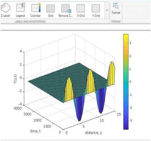
Referring to previous research related to a single rectangular plate-fin which Goeritno has implemented for making assumptions and according to a number of mathematical equations that have been obtained to diagnose the existence of the phenomenon of temperature changes, application-based simulations can be carried out. MATLAB application with an online facility is used for simulation purposes. A three-dimensional curve as an indication of the existence of the phenomenon of temperature changes is shown in Figure 5.
Based on Figure 5, it can be explained that the formation of the three-dimensional curve is based on the arrangement of syntax lines that are carried out in the command window of the MATLAB application which is accessed online.
A phenomenon of temperature change that occurs is observed along the length of the copper rod which is assumed to be 15 cm long in the form of a sinusoidal curve with the selected observation time range of up to 3,600 seconds. The assumption of the length of the copper rod for a single rectangular plate-fin and the assumption of the time span is based on previous studies by Goeritno [reference of 24th]. Based on this, it can be determined that the creation of a PDE-based mathematical model for observing the phenomenon of temperature changes that are influenced by distance and time variables based on the form of the one-dimensional heat conduction equation can be solved by the method of separating variables.
The syntax structure of the program for the formation of the three-dimensional curve is shown in Figure 6.
Figure 5. A three-dimensional curve as an indication of the existence of the phenomenon of temperature changes
Figure 6. The syntax structure of the program for the formation of the three-dimensional curve
Based on Figure 6, it can be explained that the syntax structure for programming based on MATLAB application consists of (i) initial condition, (ii) boundary condition, (iii) solving the equations, and (iv) plotting the 1-dim heat conduction equation.
Based on results and discussions can be concluded according to the research objectives. Making the prototype of the problem based on the one-dimensional heat conduction equation obtained a mass balance that developed for a finite segment $\Delta z$ along the tank’s longitudinal axis in order to derive a differential equation. Processing the solution of the mathematical equation based on parabolic PDE using the separation of variables obtained the final complete solution in the form of a Fourier sine series. Displaying the temperature changes phenomena in the form of curves is obtained as a three-dimensional curve as an indication of the existence of the phenomenon of temperature changes.
The research contribution is presented in this article explained by a clear description of the phenomenon of temperature change based on differences, that the phenomena observed through the use of the same materials and basic equations, also the observed phenomena are the same, namely observations of changes in temperature but solved in a different way. The previous solutions are based on ordinary differential equations because each independent variable is solved independently. This research is based on partial differential equations because the two independent variables are solved simultaneously by the method of separating the variables.
Suggestions for further research in the future can be used in several methods grouped in analytical methods for solving parabolic type partial differential equations in one-dimensional heat conduction cases, including the use of several methods grouped in numerical methods, especially the method of finite difference or grid.
|
PDE |
partial differential equation |
|
PDEs |
partial differential equations |
|
ODEs |
ordinary differential equations |
|
x |
independent variable; x-axis; the interval value of the lengthiness |
|
y |
independent variable; y-axis |
|
z |
independent variable; z-axis |
|
t |
time |
|
H |
heat |
|
T |
temperature |
|
B |
fin thickness |
|
L |
fin lengthiness |
|
W |
fin widths |
|
d |
differentiating with one variable |
|
$\Delta$ |
the segment of a |
|
$\Delta z$ |
distance between zi and zi+1 |
|
q |
heat flux at the surface |
|
h |
heat transfer coefficient |
|
A, B, C, D, V |
constants |
|
∂ |
differentiating with two or more variables |
|
u,f |
functions |
|
L |
lengthiness |
|
α,β |
constants of the boundary condition |
|
U |
variable of the boundary condition; over-all heat transfer coefficient |
|
h |
heat transfer coefficient |
|
k |
thermal conductivity, W.m-1. K-1 |
|
Cp |
specific heat, J. kg-1. K-1 |
|
Q |
the energy balance in the heat conduction process |
|
$\mathbb{R}$ |
the set of real numbers |
|
$\in$ |
a member of |
|
$\rightarrow$ |
implies |
|
δ |
variable of distance |
|
θ |
variable of temperature |
|
p, q, r |
continuous functions |
|
a1,a2,c,n |
contants |
|
e |
exponential number = 2.71828… |
|
G |
a coefficient in the Fourier series |
|
“A” |
area, m2 |
|
IC |
initial conditions |
|
BC |
boundary conditions |
|
Greek symbols |
|
|
ψ |
function |
|
μ |
the same constant |
|
λ |
interval of temperature |
|
π |
pi number |
|
Superscripts |
|
|
1, 2, n |
sequence to |
|
(n) |
n-th derivative |
|
Subscripts |
|
|
1, 2, n |
sequence to |
|
met. |
metal |
|
cu |
copper |
|
a |
air |
|
f |
fluid |
|
w |
wall |
|
z |
in z-axis |
[1] Cole, S. (1983). The hierarchy of the sciences? American Journal of Sociology, 89(1): 111-139. https://dx.doi.org/10.1086/227835
[2] Smith, L.D., Best, L.A., Stubbs, A., Johnston, J., Archibald, A.B. (2000). Scientific graphs and the hierarchy of the sciences. Social Studies of Science, 30(1): 73-94. https://dx.doi.org/10.1177/030631200030001003
[3] Ledoux, S.F. (2002). Defining natural sciences. Behaviorology Today, 5(1): 34-36. https://behaviorology.org/oldsite/pdf/DefineNatlSciences.pdf.
[4] Hedges, L.V. (1987). How hard is hard science, how soft is soft science? The empirical cumulativeness of research. American Psychologist, 42(5): 443-455. https://dx.doi.org/10.1037/0003-066X.42.5.443
[5] Mason, M.G. Physics: The Science of the Universe and Everything in It. Wiley University Services. https://www.environmentalscience.org/physics, accessed on March 17, 2022.
[6] Adomian, G. (1994). On Modelling Physical Phenomena. Solving Frontier Problems of Physics: The Decomposition Method. https://dx.doi.org/10.1007/978-94-015-8289-6
[7] Bueno, O., French, S. (2012). Can mathematics explain physical phenomena? The British Journal for the Philosophy of Science, 63(1): 85-113. https://www.jstor.org/stable/41410128.
[8] Ray, S.S., Bera, R.K., Kılıçman, A., Agrawal, O.P., Khan, Y. (2015). Analytical and numerical methods for solving partial differential equations and integral equations arising in physical models. Abstract and Applied Analysis, 2015: 193030. https://dx.doi.org/10.1155/2015/193030
[9] Abderezzak, B. (2018). Heat Transfer Phenomena. Introduction to Transfer Phenomena in PEM Fuel Cell. London, UK: ISTE Press - Elsevier, 125-153. htpps://dx.doi.org/10.1016/b978-1-78548-291-5.50004-4
[10] Laloui, L., Loria, A.F.R. (2020). Analytical modelling of transient heat transfer. Analysis and Design of Energy Geostructures, 409-456. htpps://dx.doi.org/10.1016/b978-0-12-816223-1.00009-6
[11] Soldatenko, S., Bogomolov, A., Ronzhin, A. (2021). Mathematical modelling of climate change and variability in the context of outdoor ergonomics. Mathematics, 9(22): 2920. https://dx.doi.org/10.3390/math9222920
[12] Choksi, R., Gonzlez, M.D.M., Gualdani, M., Schonbek, M.E. (2013). Partial differential equations in the social and life science: Emergent challenges in modeling, analysis, and computations. https://www.birs.ca/workshops/2013/13w5106/report13w5106.pdf.
[13] Pinky, M.A., (2003). Boundary-value problems in rectangular coordinates. Partial Differential Equations and Boundary-value Problems with Applications, 3rd ed. American Mathematical Society, Providence, RI, Waveland Prees, Inc., Long Grove, IL, 99-170.
[14] Zill, D.G., and Cullen, M.R. (2005). Introduction to differetial equations. Differential Equations with Boundary-Value Problems, 7th ed. Brooks/Cole, Cengage Learning, Belmont, CA, 1-34.
[15] Strauss, W.A. (2008). Partial Differential Equations: An Introduction. John Wiley & Sons, Inc., Hoboken, NJ, 1-32.
[16] Powers, D.L. (2009). The Heat Equation. Boundary Value Problems and Partial Differential Equations, 6th ed. Elsevier Academic Press, Cambridge, MA, 135-214.
[17] Boyce, W.E., and DiPrima, R.C. (2009). Partial differential equations and Fourier series. Elementary Differential Equations and Boundary Value Problems. 9th ed. John Wiley & Sons, Inc., Hoboken, NJ, 577-664.
[18] Dawkins, P. (2011). Partial Differential Equation. Differential Equation. Beaumont, TX: Lamar University, 497-554, https://tutorial.math.lamar.edu/GetFile.aspx?file=B,1,N.
[19] Yang, X.S. (2017). Partial differential equations. Engineering Mathematics with Examples and Applications. San Diego, CA, Academic Press is an imprint of Elsevier, Inc., 287-299, https://dx.doi.org/10.1016/b978-0-12-809730-4.00033-1
[20] Yu, X. (2017). Research on separation variable method in mathematical physics equation. Advances in Engineering Research, 123: 62-65.
[21] Multiphysics Cyclopedia. (2019). The laws of physics, mathematical models, and PDEs. Physics, PDEs, Mathematical and Numerical Modeling. https://www.comsol.com/multiphysics/introduction-to-physics-pdes-and-numerical-modeling, accessed on Jan. 20, 2020.
[22] Toth, A., Bobok, E. (2017). Basic equations of fluid mechanics and thermodynamics. Flow and Heat Transfer in Geothermal Systems, 21-55. https://dx.doi.org/10.1016/b978-0-12-800277-3.00002-5
[23] Bird, R.B., Stewart, W.E., Lightfoot, E.N. (1960). Transport Phenomena. John Wiley & Sons, New York, 288.
[24] Goeritno, A. (2021). Ordinary differential equations models for observing the phenomena of temperature changes on a single rectangular plate fin. Mathematical Modelling of Engineering Problems, 8(1): 89-94. https://dx.doi.org/10.18280/mmep.080111
[25] Goeritno, A. (2022). Analytical and numerical simulations to observe the seawater cooling phenomena through a single rectangular plate-fin. Mathematical Modelling of Engineering Problems, 9(1): 159-167. https://dx.doi.org/10.18280/mmep.090120
[26] Cengel, Y.A. (2007). Heat conduction equation. Heat and Mass Transfer, 3rd ed. New York City, NY: McGraw-Hill, 63-133.
[27] Krivtsov, A.M., Sokolov, A.A., Müller, W.H., Freidin, A.B. (2018). One-Dimensional Heat Conduction and Entropy Production. In: dell'Isola, F., Eremeyev, V., Porubov, A. (eds) Advances in Mechanics of Microstructured Media and Structures. Advanced Structured Materials, vol 87. Springer, Cham. https://doi.org/10.1007/978-3-319-73694-5_12
[28] Al-Mamun, A., Ali, Md.S., Miah, Md.M. (2018). A study on an analytic solution 1D heat equation of a parabolic partial differential equation and implement in computer programming. International Journal of Scientific and Engineering Research, 9(9): 913-921.
[29] Subani, N., Jamaluddin, F., Mohamed, M.A.H., Badrolhisam, A.D.H. (2020). Analytical solution of homogeneous one-dimensional heat equation with neumann boundary conditions. Journal of Physics: Conference Series, 1551: 012002. https://dx.doi.org/10.1088/1742-6596/1551/1/012002
[30] Vaidya, N.V., Deshpande, A.A., Pidurkar, S.R. (2021). Solution of heat equation (Partial Differential Equation) by various methods. International Conference on Research Frontiers in Sciences (ICRFS 2021), Nagpur, India. https://dx.doi.org/10.1088/1742-6596/1913/1/012144
[31] Bar-Sinai, Y., Hoyer, S., Hickey, J., Brenner, M.P. (2019). Learning data-driven discretizations for partial differential equations. Proceedings of the National Academy of Sciences, 116(31): 15344-15349. https://dx.doi.org/10.1073/pnas.1814058116
[32] Salih, A. (2014). Classification of partial differential equations and canonical forms. https://www.iist.ac.in/sites/default/files/people/Canonical_form.pdf, accessed on Jan. 30, 2021.
[33] Kirkwood, J. (2018). Three important equations. Mathematical Physics with Partial Differential Equations, 217-236. https://dx.doi.org/10.1016/b978-0-12-814759-7.00005-3
[34] Nordström, J., Hagstrom, T.M. (2020). The number of boundary conditions for initial boundary value problems. SIAM Journal on Numerical Analysis, 58(5): 2818-2828. https://dx.doi.org/10.1137/20m1322571
[35] Arfken, G. (1985). Mathematical Methods for Physicists, 3rd ed. Academic Press, Orlando, FL, pp. 502-504.
[36] Walet, N. (2022). Boundary and Initial Conditions. Libretexts. https://batch.libretexts.org/print/Letter/Finished/math-8309/Full.pdf, accessed on Aug. 17, 2022. [37] Asmar, N.H., (2005). Sturm-Liouville Theory with Engineering Applications. Partial Differential Equations with Fourier Series and Boundary Value Problems, 2nd ed. Prentice Hall, Upper Saddle River, NJ, 326-289.