Habiba A. Ibrahim | Hossam Hassan Ammar* | Raafat Shalaby
© 2022 IIETA. This article is published by IIETA and is licensed under the CC BY 4.0 license (http://creativecommons.org/licenses/by/4.0/).
OPEN ACCESS
The field of rehabilitation robotics for upper limb assistance has grown rapidly in the past few years. Rehabilitation robots have direct contact with human joints, which presents a serious safety concern. In this paper, a novel design for a series elastic actuator (SEA) is presented for upper limb rehabilitation of sensorimotor dysfunctions. The proposed SEA ensures safety and robust torque control under various disturbances. The proposed SEA is modeled and simulated using MATLAB Simulink to obtain Input/Output driven data. For the proposed system, two modeling approaches, ARMAX and NN, are used along with comparative analysis for each model fitting. After SEA dynamic modeling, the PSO-tuned LQR controller is designed and implemented. Comparison parameters are then chosen to test the controller behavior during different applied disturbances. The chosen controller showed optimum set-point tracking performance, which is equivalent to upper limb movement. This research can be extended to develop and implement a test bench for upper limb rehabilitation.
series elastic actuator (SEA), ARMAX, neural network (NN), LQR controller, particle swarm optimization (PSO), upper limb rehabilitation
Robots are considered as potential assistants to humans in many life aspects. The need to recruit robots in many sensitive environments that require direct interaction with humans has increased dramatically in the last few years [1]. One of the emerging fields to use robotics is the medical field, specifically where robots are used to assist the patient recovery process [2]. Recovery assisting robots fall into three main categories: end-effector manipulators assisting in hand and wrist functions, cable driven robot that mobilizes the targeted limb through cables driven via motors, and exoskeleton that acts parallel to the moving limb [3]. Each of these architectures involves direct contact to a human body part that does not tolerate any unexpected motion error. Different approaches were followed to apply the optimum actuation technique that ensure safe human-robot interaction [4]. Regarding exoskeleton robots, research aimed to minimize the weight and the bulkiness of the device attached to the affected limb. One of the solutions was to use soft pneumatic powered muscles instead of rigid motors. Pneumatic muscle actuators (PAM) are considered as compliance actuators as it contains soft elements, as well as having high power-to-weight ratio [5, 6].
In rehabilitation field, the continuous research aims to enhance the reaction of the used robotic assisting devices with the motion of human joints [7]. Elastic actuators provide the compliance concept that ensures high safety measures and comfort functionalities [8]. Series Elastic Actuator (SEA) is a type of Variable Impedance Actuator (VIA) and was first introduced in 1995 [9]. SEA is recognized as high-performance torque control as well as high force generation [10]. Unlike rigid actuators, SEA uses the deflection of the elastic element as the spring to generate the required torque instead of being transmitted through the gearbox [11]. The structure of SEA offers precise force and velocity controls; however, the elastic element cause lack of position accuracy.
The complexity of such system can be in choosing an accurate modeling technique that will capture the system non-linearities and uncertainties. One of the powerful models is Artificial Neural Network (ANN) which is designed to simulate the working mechanism of the human brain in analyzing data. ANN is one technique of Artificial Intelligence (AI) that has the capability of self-learning and predicting the behavior of the system. ANN has become useful in multiple fields such as health care professions in which ANN has been used to predict certain diseases. Also, in fields such as predicting the behavior and efficiency of electromechanical system that are non-linear systems.
Improvements done to SEA by Sensinger and Weir included having precise force control to increase safety while interacting with humans. This could be achieved by various methods such as using inertia reduction, joint torque control, and passive impedance modulations [12]. Another trial for the accurate controller on SEA was done by Wyeth. He introduced using the motor as a velocity source instead of being a torque source, this will allow having an internal velocity feedback loop. The experiments showed improvements in SEA performance while using cascaded Proportional Integral (PI) controllers. This method was also used to control the haptic manipulators by having accurate force control with high safety [13]. The same cascaded controller was used in addition to an inner velocity loop to control haptic manipulators [14]. The approach resulted in more accurate force tracking.
Due to the existence of elastic elements in series with the rigid motor, system behavior includes uncertainties and oscillations. Considering the sensitivity of SEA applications, designing a robust controller is crucial. Obtaining an accurate dynamic model is the initial step to design the desired controller. An adaptive controller enables the system to update the corresponding parameters online based on the changes in the operating conditions [15]. For SEA, the conventional controllers such as Proportional Integral Derivative (PID) fail to achieve accurate trajectory for dynamic joints, an adaptive controller using Radial basis function (RBF) neural network is proposed by Shao et al. [16]. A similar algorithm was used in Ref. [17] to predict and model muscle behavior to ensure safe interaction between the artificial joint and the human body. In [15], adaptive immersion and invariance (I\&I) are used to control the system relative to the varying operating parameters. Another technique is presented by Fotuhi and Bingul [18] to use feedforward PID controller, feedforward fuzzy controller, and fuzzy torque controller with friction compensation with an illustrative comparison.
For the proposed SEA, two modeling techniques are presented along with a comparative analysis for the accuracy of system identification. System identification is conducted using Auto-Regressive Moving Average eXogenous model (ARMAX) for linear modeling, and for nonlinear modeling an Artificial Neural Network (ANN) technique is used. ARMAX model is mainly defined as a Single Input Single Output (SISO) model as it can be used to control single oscillation mode, yet it is used to model Multi Input Multi Output (MIMO) systems containing disturbances [19, 20]. Following the system modeling, a controller design phase took place. The proposed system controller is based on initially using Linear Quadratic Regulator (LQR) controller, then parameters' refinement is done using Particle Swarm Optimization (PSO) algorithm.
This paper is organized as follows: the proposed SEA design and system dynamic modeling are illustrated in section 2. Sections 3 and 4 present the followed techniques of linear and non-linear modeling, along with comparative analysis of the three techniques. After system modeling, section 5 illustrates the designed controller for the system. The reached results were discussed in section 6.
2.1 Design of series elastic actuator
SEA is a rigid actuator that includes an elastic element at the output side of the motor. Reducing the stiffness of the actuator helps solve several problems such as backlash, and friction. There are various types of SEA, categorized based on the location of the elastic element within the actuation system. SEA configurations include the force sensing type (FSEA), the transmission force-sensing type (TFSEA), and the reaction force-sensing type (RSEA) [21].
The FSEA categorization has the elastic element directly before the load side. The proposed model includes elastic elements as four springs with equal coefficients connected to a movable arm. The arm with the elastic elements is moved by the motor through a lead screw. The load then can act on the other side of the system and the deflection in the springs will happen accordingly. Table 1 shows a comparative study conducted on different SEA designs regarding the main design characteristics.
Table 1. Characteristic features of selected robotic devices
|
Published study |
Range of motion restriction |
Mechanical impedance |
Power transmission |
Joint misalignment |
Total weight |
|
[22] |
The device does not interfere with the natural range of motion. |
Mechanical impedance is kept to the minimum due to the DC motor and the compliant element stiffness. |
The torque is transmitted through a cable to relocate the motor away from the joint. |
Due to the relocation of the motor, no misalignment has occurred. |
Not specified |
|
[23] |
The system allows range of rotation equal to 93 for elbow joint. |
The stiffness of the linear spring reduces the mechanical impedance of the system. |
The torque is transmitted from the motor to a linear guide and to the joint via slider crank mechanism. |
The motor is attached to the joint, so there is misalignment. |
1.7 kg. |
|
[24] |
No interference with the natural range of motion. |
The cable selection provides low friction and minimized impedance. |
Torque is transmitted via flexible cable due to relocation away from the joint. |
No misalignment as the motor is not fixed on the joint. |
Not specified. |
|
[25] |
The SEA provides enough frequency to assist the movement of human joint. |
The usage of DC servo motor decreases the movement inertia to the minimum. |
The torque is transmitted through Bowden cable. |
No experiment on human joint was conducted. |
0.95 kg. |
|
[26] |
The design allows up to 180 degrees for the elbow joint rotation. |
The non-linearity of the designed stiffness is very low at the natural position, so the mechanical impedance is low. |
The torque of each motor is transmitted to the end effector through a flexible Bowden cable. |
The system is attached parallel to the elbow joint, so no misalignment occurred. |
0.9 kg. |
|
[27] |
No restriction on the movement were mentioned. |
The selected motor free shaft rotation during the Free Motion. |
Power is transmitted through gearbox and belt. |
No misalignment as the motor is not fixed on the joint. |
Not specified. |
2.2 Dynamic model
The dynamics of the actuator are derived to simulate the model and study its behavior. The dynamic model of the system consists of three main parts; the stepper motor model, the lead screw transmitting the torque, and the mechanical system attached to the motor.
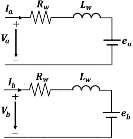
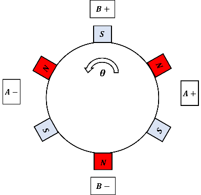
The 2-phase stepper motor dynamic model consists of mechanical equations and electrical equations. The electrical circuit diagram for each phase is shown in Figure 1. Each phase can be solved using RL circuit in addition to a back electromotive force (emf) representing phase one as a and phase two as b. The working principle of a two-phase motor can be described as if the rotor in Figure 2 is not magnetized. whenever one phase is energized, the rotor will rotate either clockwise or counterclockwise to align with the rotor teeth with the energized phase.
Figure 1. Schematic view of motor winding circuits
Figure 2. Phase distribution of a two-phase stepper motor
The mathematical model for the electrical part of the stepper motor is derived based on the following equations:
$e_{a}=-k_{m} \omega \sin \left(\theta N_{r}\right)$ (1)
$e_{b}=k_{m} \omega \cos \left(\theta N_{r}\right)$ (2)
$\frac{d i_{a}(t)}{d t}=\left(k_{m} \omega \sin (\theta p)+V_{a}-R_{w} i_{a}\right) / L_{w}$ (3)
where, ea and eb are the emf values for each phase winding, ia and ib are the phases current, km is motor torque constant, ω is the angular speed of the rotor, θ is the mechanical angle of the motor, p is the number of rotor teeth, R is the rotor resistance, and L is rotor inductance.
$\frac{d}{d t} i_{b}(t)=\left(k_{m} \omega \sin (\theta p)+V_{b}-R_{w} i_{a}\right) / L_{w}$ (4)
$V_{a}=V_{m} \sin \left(\theta p+\lambda+\frac{\pi}{2}\right)$ (5)
where, Va is the phase voltage, Vm is the input voltage, and λ is phase shifts.
$V_{b}=V_{m} \sin (\theta p+\lambda)$ (6)
For the mechanical equations:
$J \frac{d}{d t} \omega(t)=-T_{l}+i_{a} k_{m} \sin (\theta p)-i_{b} k_{m} \cos (\theta p)$ (7)
where, J is the moment of inertia, and Tl is the load torque amplitude. Each phase in Figure 2 has a corresponding static torque represented by Ta and Tb. Each torque component has a contribution in the average torque value Tavr. The torque generated from each phase is calculated as follows:
$T_{a}=k i_{a} \cos (\theta p)$ (8)
$T_{b}=-k i_{b} \cos (\theta p)$ (9)
The average torque generated by the motor is calculated as follows:
$T_{a v r}=\frac{T_{a}+T_{b}}{2}$ (10)
The next part of the system is the lead screw attached to the motor shaft. Using the result of Eq. (10), the moving force Fm acting on the middle plate M2 is calculated as follows:
$F_{m}=\frac{2 \pi n 1000 T_{a v r}}{N}$ (11)
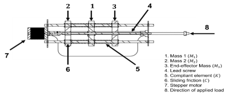
where, n is the speed in (rpm), and N is the lead screw pitch in (mm). The physical model for the proposed system is modeled as a mass-spring system and the acting forces are shown in Figure 3.
The equation of motion for both masses are calculated as follows:
$\left(M_{2}+M_{3}\right) \ddot{x}_{2}-2 C_{1} \dot{x}_{1}+\left(2 C_{1}+C_{2}\right) \dot{x}_{2}$
$-4 k\left(x_{1}-x_{2}\right)=F_{\text {load }}$ (12)
where, Mi is the mass for the corresponding plate, $\ddot{x}_{i}, \dot{x}_{i}$ and xi are respectively the acceleration, speed, and displacement of each mass, C3 is the friction coefficient from the moving rods, K is the spring stiffness, and Fload is the force from the applied load. As shown, M1 is the middle plate on which Fm acts directly. The equation of motion for both masses are calculated as follows:
$M_{1} \ddot{x}_{1}+2 C_{1}\left(\dot{x}_{1}-\dot{x}_{2}\right)+4 k\left(x_{1}-x_{2}\right)=F_{m}$ (13)
where, Fm is the moving force acting on the middle plate. This force is calculated based on the parameters of the motor and the lead screw. C1 and C2 are the friction coefficients from the rod movement that acts as dampers in the system.
Figure 3. Schematic view of the proposed SEA design
As the proposed system has multiple inputs and outputs, it is required to minimize the order of the system’s differential equations using state-space representation. Eq. (14) shows the genral form of state-space representation. To derive the state-space model, the variables can be defined in more subtle representation as follows:
$\dot{x}(t)=A x(t)+B u(t)$
$y(t)=C x(t)+D u(t)$ (14)
where, A is the state matrix, B is the input matrix, y is the system output, C is the output matrix, and D is the direct transition matrix.
To derive the state-space model, define the state vector $z=\left[\begin{array}{llll}x_{1} & v_{1} & x_{2} & v_{2}\end{array}\right]^{T}$ where, $v_{1}=\dot{x}_{1}$ and $v_{2}=\dot{x}_{2}$.
Rearranging Eqns. (12) and (13), we obtain:
$\dot{v}_{1}=-\frac{4 k}{M_{1}} x_{1}-\frac{2 C_{1}}{M_{1}} v_{1}+\frac{4 k}{M_{1}} x_{2}+\frac{2 C_{1}}{M_{1}} v_{2}+\frac{1}{M_{1}} F_{m}$ (15)
$\begin{aligned} \dot{v}_{2}=\frac{4 k}{M_{2}+M_{3}} x_{1} &+\frac{2 C_{1}}{M_{2}+M_{3}} v_{1}-\frac{4 k}{M_{2}+M_{3}} x_{2} \\ &-\frac{2 C_{1}-C_{2}}{M_{2}+M_{3}} v_{2}+\frac{1}{M_{2}+M_{3}} F_{l o a d} \end{aligned}$ (16)
State-space representation for a system is given by the following equations. Forming the state-space equations for the proposed system is shown in Eq. (19) and Eq. (20).
where, the state matrix A and the input matrix B will be as follows:
$A=\left[\begin{array}{llll}0 & 1 & 0 & 0 \\ \frac{-4 k}{M_{1}} & \frac{-2 C_{1}}{M_{1}} & \frac{4 k}{M_{1}} & \frac{2 C_{1}}{M_{1}} \\ 0 & 0 & 0 & 1 \\ \frac{4 k}{M_{2}+M_{3}} & \frac{2 C_{1}}{M_{2}+M_{3}} & \frac{-4 k}{M_{2}+M_{3}} & \frac{C_{2}-2 C_{1}}{M_{2}+M_{3}}\end{array}\right]$ (17)
$B=\left[\begin{array}{lll}0 & 0 & \\ \frac{1}{M_{1}} & 0 & \\ 0 & 0 & \\ 0 & \frac{1}{M_{2}+M_{3}}\end{array}\right]$ (18)
$\left[\begin{array}{l}\dot{x}_{1} \\ \dot{v}_{1} \\ \dot{x}_{2} \\ \dot{v}_{2}\end{array}\right]=\left[\begin{array}{llll}0 & 1 & 0 & 0 \\ \frac{-4 k}{M_{1}} & \frac{-2 C_{1}}{M_{1}} & \frac{4 k}{M_{1}} & \frac{2 C_{1}}{M_{1}} \\ 0 & 0 & 0 & 1 \\ \frac{4 k}{M_{2}+M_{3}} & \frac{2 C_{1}}{M_{2}+M_{3}} & \frac{-4 k}{M_{2}+M_{3}} & \frac{C_{2}-2 C_{1}}{M_{2}+M_{3}}\end{array}\right]\left[\begin{array}{l}x_{1} \\ v_{1} \\ x_{2} \\ v_{2}\end{array}\right]+\left[\begin{array}{ll}0 & 0 \\ \frac{1}{M_{1}} & 0 \\ 0 & 0 \\ 0 & \frac{1}{M_{2}+M_{3}}\end{array}\right]\left[\begin{array}{l}F_{m} \\ F_{l o a d}\end{array}\right]$ (19)
$y=\left[\begin{array}{llll}1 & 0 & 0 & 0 \\ 0 & 1 & 0 & 0 \\ 0 & 0 & 1 & 0 \\ 0 & 0 & 0 & 1\end{array}\right]\left[\begin{array}{l}x_{1} \\ v_{1} \\ x_{2} \\ v_{2}\end{array}\right]$ (20)
as xi and vi is the displacement and velocity corresponding to each mass, respectively.
2.3 Motion analysis
To study the actuator behavior under various cases, the CAD model shown in Figure 4 is tested and simulated under different constraints and conditions. SolidWorks is used to create a motion study that includes motor rotational speed, values for stiffness coefficients, and the applied load. As the proposed actuator is mainly designed to be used in upper limb rehabilitation robotics, the acting force on the actuator is calculated as follows:
$F_{\text {load }}=m_{\text {arm }} g \sin \theta$ (21)
where, marm is the forearm mass, g is the gravitational acceleration, $\theta$ is the elbow angle ranging from 30° to 150°.
Regarding the spring coefficients, different random spring constants were chosen to study the effect of relatively high and low stiffness on the system behavior. Taking in consideration the standard vale ranges available in the local market. Similarly, a set of values regarding the motor rotational speed were used, and the system response was recorded for each trial.
As the proposed actuator is mainly designed to be used in upper limb rehabilitation robotics, the actuator has to perform passive and active motion assisting the elbow joint. Upper limb muscles act in pairs as flexors and extensors.
Figure 4. CAD model for the proposed SEA
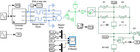
Figure 5. Schematic overview for the proposed system structure
The flexor is the biceps muscle that moves to close the upper limb, and the extensor is the triceps muscle that opens the upper limb [28]. The actuator will operate while taking into consideration the angle of the elbow joint only. The angle of the shoulder complex will not affect the operation of the actuator, as the motion will be either flexion or extension of the elbow joint. According to the study [29], the average forearm mass range is 2.1 kg if the average mass of a whole body is 70 kg as the mass of the arm represents about 2.2% of the total body mass. As the arm will not be holding any other object, so the weight of the forearm itself is the only force acting on the actuator. Eq. (21) represents the load force caused by forearm movement.
Figure 6 shows the total stroke length while changing the values of both stiffness coefficients and motor angular velocity. In the figure, the chosen values are shown in Table 2.
Figure 6. Displacement of actuator stroke
Table 2. Motion analysis trials
|
Test values |
Trial no. |
|||
|
Trial 1 |
Trial 2 |
Trial 3 |
Trial 4 |
|
|
Stiffness Coefficients (N/mm) |
50 |
50 |
100 |
100 |
|
Motor Velocity (rpm) |
150 |
350 |
350 |
150 |
3.1 System identification
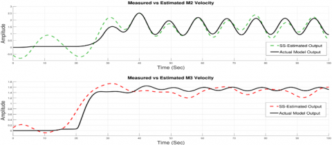
System identification is an engineering method that helps to determine and derive the mathematical model for a system using the measured data. Using the system representation in Figure 5 the needed data for identification was generated. Table 3 shows the applied simulation parameters. The whole system is considered a Multiple Input Multiple Output (MIMO) system as it has two inputs and two outputs. The inputs for the system are the motor speed and PWM and the outputs are the velocity of M2 and M3. System state space is estimated based on imported inputs and outputs. The unknown variables and parameters of the analytical state-space with step input are estimated to be as follows:
$A=\left[\begin{array}{llll}0.982 & 0.01388 & -0.01608 & -0.05286 \\ -0.01316 & 0.7825 & -0.05617 & 0.06703 \\ 0.06557 & 0.07432 & 0.9877 & 0.01564 \\ 0.02461 & -0.2487 & 0.0568 & 0.813\end{array}\right]$
$B=\left[\begin{array}{ll}0 & 0 \\ 0.1918 & 0 \\ 0 & 0 \\ 0 & 0.000223\end{array}\right]$
$C=\left[\begin{array}{llll}4.849 & 0.2082 & -0.05421 & -0.1429 \\ 3.352 & 3.409 & -0.1902 & 0.0202\end{array}\right]$
$K=\left[\begin{array}{ll}0.1609 & -0.02134 \\ -0.1962 & 0.2114 \\ -0.1063 & -0.4791 \\ -1.165 & 0.4828\end{array}\right]$
The estimated model resulted in fitting accuracy equals 0.530 for the first output and 0.728 for the second output, as shown in Figure 7. The graph shows the agreement between validation outputs and model outputs.
Table 3. Simulation parameters for simulink model
|
Parameters |
Value |
|
M1, M2, M3 |
0.2 kg |
|
C |
0.01 N/(m/s) |
|
K |
0.01 N/m |
|
Rotor inertia |
0.45 g*m2 |
|
Maximum step rate |
50 Hz |
|
Full step size |
1.8 deg |
Figure 7. Measured and simulated system outputs of state space model
4.1 ARMAX
System modeling is defined in terms of transfer functions and differential equations. A generic linear model is represented in Eq. (22):
$y(t)=G(q) u(t)+H(q) v(t)$ (22)
where, G(q) is the input function, u(t) relates the input to the output y(t), and H(q) is the noise function which relates the noise signal v(t) to the output y(t).
ARMAX is one of the simpler models for parametric model estimation. ARMAX is an extension of Autoregressive with exogenous input (ARX) as it includes disturbance dynamics. ARMAX model is useful in cases when noises enter the system at the input [30]. The system model is described in ARMAX form as follows:
$A(q) y(t)=B(q) u(t)+C(q) e(t)$ (23)
where, y(t) is the measured system output; u(t) represents the exogenous system input; e(t) is the disturbance or noises on the system; q-1 is the shift operator.
The polynomial in Eq. (23) are defined as follows [31]:
$A_{a}\left(q^{-1}\right)=1+a_{1} q^{-1}+\cdots+a_{n_{a}} q^{-n_{a}}$
$B_{b}\left(q^{-1}\right)=b_{0}+b_{1} q^{-1}+\cdots+b_{n_{b}} q^{-n_{b}}$
$C_{c}\left(q^{-1}\right)=1+c_{1} q^{-1}+\cdots+c_{n_{c}} q^{-n_{c}}$
where, a1, ⋯, an are parameters of the Autoregressive part (AR), and n is the order of AR. The predictor equation for ARMAX is:
$\hat{y}(t \mid t-1)=\frac{B(q)}{C(q)} u(t)+\left(1-\frac{A(q)}{C(q)}\right) y(t)$ (24)
The prediction error is calculated as follows:
$e(t)=\frac{A(q)}{C(q)} y(t)-\frac{B(q)}{C(q)} u(t)$ (25)
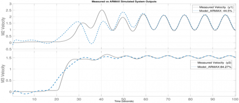
The ARMAX non-linear model is built using MATLAB embedded functions along with the generated data set. Figure 8 shows the fitting accuracy of the ARMAX model compared with the actual measured data.
Figure 8. Measured and simulated system outputs of ARMAX model
4.2 Artificial neural network (ANN)
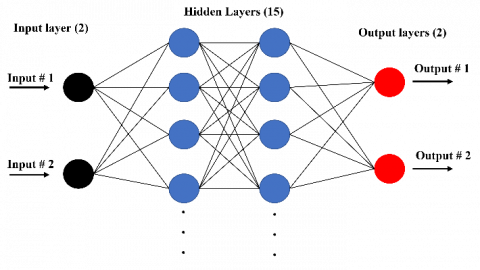
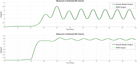
Considering the system to be MIMO system, a suitable Artificial Neural Network (ANN) model is used to capture the system's nonlinearity. The ANN is one of the examples that are capable of estimating the non-linear phenomenon in a generated data set. ANN models are known to be a powerful tool in predicting a large class of nonlinear problems due to the parallel processing. The ANN type used in this application is feedforward netwek with backpropagation. Table 4 shows the paramters of the designed ANN model. A two input layers, two output layers, and 15 hidden layers ANN model has been used as shown in Figure 9. The network is trained using MATLAB with the Levenberg-Marquardt training algorithm. Figure 10 shows the obtained results from the training process on the generated data.
Table 4. ANN design paramters
|
Training algorithm |
Levenberg-Marquardt |
|
Number of input layers |
2 |
|
Number of output layers |
2 |
|
Number of hidden layers |
15 |
|
Number of epochs |
3000 |
|
Training ratio |
70/100 |
|
Validation ratio |
15/100 |
Figure 9. Structure of ANN with two input layers, two output layers, 15 hidden layers
Figure 10. Measured and simulated system outputs of ANN model
Before proceeding with the controller design step, the controllability analysis for the system should be conducted. The rank of the controllability matrix is calculated from system state space as follows:
$\operatorname{rank}(Q)=\left[\begin{array}{llll}B & A B & A^{2} B & A^{3} B\end{array}\right]$ (26)
5.1 Linear quadratic regulator (LQR)
As a result of the analysis, the controllability matrix has full rank, thus, all four states are controllable. The objective of the proposed system is to follow the desired reference input using an appropriate controller. Based on the state space, Eq. (14), the cost function for the system is assumed to be as follows:
$J=\frac{1}{2} \int_{0}^{t}\left(x^{T} Q x+u^{T} R u\right) d t$ (27)
where, Q is the semi-definite weight matrix and R is the symmetric weight matrix of state matrix x(t) and input matrix u(t). Obtaining a solution for the previous cost function is achieved using Riccati’s equation as follows:
$P A+A^{T} P-P B R^{-1} B^{T} P+Q=0$ (28)
As the main objective of LQR control is to obtain values for Q and R weight matrices, the Riccati’s Eq. (28) can be used in the case of having a simple SISO system. For the proposed MIMO system, obtaining the same values for the weighting matrices is challenging task, which may require an optimization algorithm [31].
5.2 Particle swarm optimization (PSO)
The PSO is a simple tuning algorithm that mimics the behavior of living organisms, such as bird flocks. PSO is known for robustness in action, high efficiency that can be achieved with lower computational time compared to other metaheuristic algorithms [32]. The optimization strategy of PSO starts with the population initialization step, then each particle will search for a final solution within the pre-determined range. The next step is to find the best solution, which depends on two factors: the global best and the local best. Calculating the global best with respect to all swarm individuals based on their past success experience is shown in Eq. (29).
Table 5. PSO simulation paramters
|
Parameters |
Value |
|
Swarm size |
10 |
|
Number of iterations |
1000 |
|
Number of dimensions |
2 |
|
Lower band |
[1,1] |
|
Upper band |
[100,100] |
$v_{i}^{k+1}=h \times v_{i}^{k}+c_{1} \times \operatorname{rand} \times\left(x_{i}^{b}-x_{i}^{k}\right) c_{2} \times$rand $\times\left(x_{i}^{g}-x_{i}^{k}\right)$ (29)
The best solution resulted from the optimization process is calculated as follows:
$x_{i}^{k+1}=x_{i}^{k}+v_{i}^{k+1}$ (30)
Table 5 shows the used simulation PSO parameters for applying the optimization algorithm to find the values of Q and R controller values.
To find the optimum modeling approach, a comparative analysis is done for the used linear and non-linear modeling techniques. Figures 8 and 10 show the obtained values from each modeling approach. It is clearly seen that ANN model achieves higher fitting accuracy values for both system outputs. Another comparison approach was to calculate the error or each output for both simulated models. Tables 6 presents the RMSE and other statistical parameters of each output for ANN and ARMAX models, respectively.
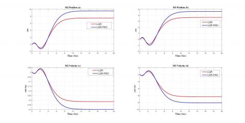
For SEA controller design, Figure 11 shows the results of applying both LQR controller and PSO-tuned LQR controller. A comparative analysis is conducted on both results based on Integral Square Error (ISE) and the weighted sum method is shown in Table 7. Based on the followed control approach, it was noticed that the PSO-tuned LQR controller is more robust as the system reached the set point faster than using only LQR controller.
Table 6. Statistical analysis for ANN and ARMAX models
|
Model Output |
Mean |
SD |
MAE |
RMSE |
NRMSE |
PearsonRp |
SpearmanRs |
|
M2 Velocity (ANN) |
1.1494 |
0.6980 |
0.1882 |
0.2684 |
0.2376 |
0.9330 |
0.8881 |
|
M3 Velocity (ANN) |
1.1737 |
0.6242 |
0.0335 |
0.0612 |
0.0612 |
0.9952 |
0.8929 |
|
M2 Velocity (ARMAX) |
1.1298 |
0.7449 |
0.2762 |
0.3689 |
0.3242 |
0.8686 |
0.6797 |
|
M3 Velocity (ARMAX) |
1.1745 |
0.6183 |
0.0422 |
0.0603 |
0.0511 |
0.9953 |
0.8197 |
Figure 11. Results of applying PSO tuned LQR controller on: (a) center mass position, (b) end-effector position, (c) center mass velocity, and (d) end-effector velocity
Table 7. Comparison between LQR and LQR-PSO
|
Controller |
ISE |
Weighted Sum Method |
|
LQR |
1539.6 |
352.79 |
|
LQR-PSO |
1695.3 |
355.07 |
An innovative SEA for upper limb rehabilitation was introduced in this research work. The proposed actuator design consists of linear springs utilized with a stepper motor to provide more precise position and velocity control. The proposed design is categorized as FSEA based on the spring placement between the motor and the applied load. The system was simulated while applying various load signals to study the system behavior. For the proposed SEA, three different modeling techniques were used based on input/output-driven data. A robust controller was designed to control the proposed SEA motion relative to the applied load signal. The controller was then tuned using PSO to obtain optimum values for LQR weight matrices. For future work, an optimization on the overall design to minimize the total weight of the system. An experimental setup will be developed for the optimized design to test the system behavior for further research.
[1] Iyer, S.S. (2012). Modeling and testing of a series elastic actuator with controllable damping. Ph.D. dissertation, Worcester Polytechnic Institute. http://dx.doi.org/10.5772/63573
[2] Wu, K.Y., Su, Y.Y., Yu, Y.L., Lin, K.Y., Lan, C.C. (2017). Series elastic actuation of an elbow rehabilitation exoskeleton with axis misalignment adaptation. In 2017 International Conference on Rehabilitation Robotics (ICORR), London, UK, pp. 567-572. http://dx.doi.org/10.1109/ICORR.2017.8009308
[3] Trigili, E., Crea, S., Moisè, M., Baldoni, A., Cempini, M., Ercolini, G., Marconi, D., Posteraro, F., Carrozza, M.C., Vitiello, N. (2019). Design and experimental characterization of a shoulder-elbow exoskeleton with compliant joints for post-stroke rehabilitation. IEEE/ASME Transactions on Mechatronics, 24(4): 1485-1496. http://dx.doi.org/10.1109/TMECH.2019.2907465
[4] Yu, H., Huang, S., Chen, G., Pan, Y., Guo, Z. (2015). Human–robot interaction control of rehabilitation robots with series elastic actuators. IEEE Transactions on Robotics, 31(5): 1089-1100. https://doi.org/10.1109/TRO.2015.2457314
[5] Chen, C.T., Lien, W.Y., Chen, C.T., Wu, Y.C. (2020). Implementation of an upper-limb exoskeleton robot driven by pneumatic muscle actuators for rehabilitation. Actuators, 9(4): 106. http://dx.doi.org/10.3390/act9040106
[6] Andrikopoulos, G., Nikolakopoulos, G., Manesis, S. (2011). A survey on applications of pneumatic artificial muscles. In 2011 19th Mediterranean Conference on Control & Automation (MED), Corfu, Greece, pp. 1439-1446. http://dx.doi.org/10.1109/MED.2011.5982983
[7] Zhang, Q., Kim, K., Sharma, N. (2019). Prediction of ankle dorsiflexion moment by combined ultrasound sonography and electromyography. IEEE Transactions on Neural Systems and Rehabilitation Engineering, 28(1): 318-327. http://dx.doi.org/10.1109/TNSRE.2019.2953588
[8] Zhang, Q., Sun, D., Qian, W., Xiao, X., Guo, Z. (2020). Modeling and control of a cable-driven rotary series elastic actuator for an upper limb rehabilitation robot. Frontiers in Neurorobotics, 14: 13. http://dx.doi.org/10.3389/fnbot.2020.00013
[9] Vanderborght, B., Albu-Schäffer, A., Bicchi, A., et al. (2013). Variable impedance actuators: A review. Robotics and Autonomous Systems, 61(12): 1601-1614. http://dx.doi.org/10.1016/j.robot.2013.06.009
[10] Lee, C., Kwak, S., Kwak, J., Oh, S. (2017). Generalization of series elastic actuator configurations and dynamic behavior comparison. Actuators, 6(3): 26. http://dx.doi.org/10.3390/act6030026
[11] Li, X., Pan, Y., Chen, G., Yu, H. (2016). Adaptive human–robot interaction control for robots driven by series elastic actuators. IEEE Transactions on Robotics, 33(1): 169-182. http://dx.doi.org/10.1109/TRO.2016.2626479
[12] Robinson, D.W. (2000). Design and analysis of series elasticity in closed-loop actuator force control. Ph.D. dissertation, Massachusetts Institute of Technology.
[13] Wyeth, G. (2006). Control issues for velocity sourced series elastic actuators. In Proceedings of the 2006 Australasian Conference on Robotics and Automation. Australian Robotics and Automation Association, pp. 1–6.
[14] Vallery, H., Ekkelenkamp, R., Van Der Kooij, H., Buss, M. (2007). Passive and accurate torque control of series elastic actuators. In 2007 IEEE/RSJ International Conference on Intelligent Robots and Systems, San Diego, CA, USA, pp. 3534-3538. http://dx.doi.org/10.1109/IROS.2007.4399172
[15] Chen, K., Astolfi, A. (2018). I&I adaptive control for systems with varying parameters. In 2018 IEEE Conference on Decision and Control (CDC), Miami, FL, USA, pp. 2205-2210. http://dx.doi.org/10.1109/CDC.2018.8619564
[16] Shao, N., Zhou, Q., Shao, C., Zhao, Y. (2021). Adaptive control of robot series elastic drive joint based on optimized radial basis function neural network. International Journal of Social Robotics, 13(7): 1823-1832. https://doi.org/10.1007/s12369-021-00762-0
[17] Liao, C., Ma, H., Wu, H. (2019). Adaptive Control of Series Elastic Actuator Based on RBF Neural Network. In 2019 Chinese Automation Congress (CAC), Hangzhou, China, pp. 4365-4369. http://dx.doi.org/10.1109/CAC48633.2019.8996349
[18] Fotuhi, M.J., Bingul, Z. (2021). Fuzzy torque trajectory control of a rotary series elastic actuator with nonlinear friction compensation. ISA Transactions, 115: 206-217. https://doi.org/10.1016/j.isatra.2021.01.020
[19] Moore, S.M., Lai, J.C.S., Shankar, K. (2007). ARMAX modal parameter identification in the presence of unmeasured excitation—I: Theoretical background. Mechanical Systems and Signal Processing, 21(4): 1601-1615. http://dx.doi.org/10.1016/j.ymssp.2006.07.003
[20] Chen, T., Lou, J., Yang, Y., Ma, J., Li, G., Wei, Y. (2018). Auto-regressive moving average with exogenous excitation model based experimental identification and optimal discrete multi-poles shifting control of a flexible piezoelectric manipulator. Journal of Vibration and Control, 24(24): 5707-5725. http://dx.doi.org/10.1177/1077546318790866
[21] Lee, C., Oh, S. (2016). Configuration and performance analysis of a compact planetary geared elastic actuator. In IECON 2016-42nd Annual Conference of the IEEE Industrial Electronics Society, Florence, Italy, pp. 6391-6396. http://dx.doi.org/10.1109/IECON.2016.7793816
[22] Blumenschein, L.H., McDonald, C.G., O'Malley, M.K. (2017). A cable-based series elastic actuator with conduit sensor for wearable exoskeletons. In 2017 IEEE International Conference on Robotics and Automation (ICRA), pp. 6687-6693. http://dx.doi.org/10.1109/ICRA.2017.7989790
[23] Wu, K.Y., Su, Y.Y., Yu, Y.L., Lin, K.Y., Lan, C.C. (2017). Series elastic actuation of an elbow rehabilitation exoskeleton with axis misalignment adaptation. In 2017 International Conference on Rehabilitation Robotics (ICORR), London, UK, pp. 567-572. http://dx.doi.org/10.1109/ICORR.2017.8009308
[24] Zhang, Q., Sun, D., Qian, W., Xiao, X., Guo, Z. (2020). Modeling and control of a cable-driven rotary series elastic actuator for an upper limb rehabilitation robot. Frontiers in Neurorobotics, 14: 13. http://dx.doi.org/10.3389/fnbot.2020.00013
[25] Zhang, Q., Xu, B., Guo, Z., Xiao, X. (2017). Design and modeling of a compact rotary series elastic actuator for an elbow rehabilitation robot. In International Conference on Intelligent Robotics and Applications, pp. 44-56. http://dx.doi.org/10.1007/978-3-319-65298-6_5
[26] Chen, T., Casas, R., Lum, P.S. (2019). An elbow exoskeleton for upper limb rehabilitation with series elastic actuator and cable-driven differential. IEEE Transactions on Robotics, 35(6): 1464-1474. http://dx.doi.org/10.1109/TRO.2019.2930915
[27] DeBoon, B., Nokleby, S., La Delfa, N., Rossa, C. (2019). Differentially-clutched series elastic actuator for robot-aided musculoskeletal rehabilitation. In 2019 International Conference on Robotics and Automation (ICRA), Montreal, QC, Canada, pp. 1507-1513. http://dx.doi.org/10.1109/ICRA.2019.8793586
[28] Erdemir, A., McLean, S., Herzog, W., van den Bogert, A.J. (2007). Model-based estimation of muscle forces exerted during movements. Clinical Biomechanics, 22(2): 131-154. http://dx.doi.org/10.1016/j.clinbiomech.2006.09.005
[29] Raikova, R. (1992). A general approach for modelling and mathematical investigation of the human upper limb. Journal of Biomechanics, 25(8): 857-867. http://dx.doi.org/10.1016/0021-9290(92)90226-Q
[30] Rangasamy, K. (2014). System identification for SISO systems. Universiti Teknologi PETRONAS. http://utpedia.utp.edu.my/id/eprint/14190.
[31] Hasan, N.S., Rosmin, N., Khalid, S., Osman, D.A.A., Ishak, B., Mustaamal, A.H. (2017). Harmonic suppression of shunt hybrid filter using LQR-PSO based. International Journal of Electrical and Computer Engineering (IJECE), 7(2): 869-876. http://dx.doi.org/10.11591/ijece.v7i2.pp869-876
[32] Azar, A.T., Ammar, H.H., Ibrahim, Z.F., Ibrahim, H.A., Mohamed, N.A., Taha, M.A. (2019). Implementation of PID controller with PSO tuning for autonomous vehicle. In International Conference on Advanced Intelligent Systems and Informatics, pp. 288-299. https://doi.org/10.1007/978-3-030-31129-2_27