Isti Fadah* | Anis Elliyana | Yudha Alif Auliya | Yustri Baihaqi | Muhammad Haidar | Dhea Milinia Sefira
© 2022 IIETA. This article is published by IIETA and is licensed under the CC BY 4.0 license (http://creativecommons.org/licenses/by/4.0/).
OPEN ACCESS
Companies engaged in agro-industry, such as rice seed companies, depend on an efficient distribution process because of the characteristics of rice seed products that are easily damaged and do not last long. The distribution and delivery of goods from the production plant to reach consumers must go through several local distributors in several areas (multi-level) such as distributor centers, retailers, and agents spread across several cities in East Java Province. Determining the distribution network will be more complex when a company produces more than one type of product (multiproduct). Based on previous research, the genetic algorithm (GA) has been proven to provide the best solution for various optimization and combinatorial problems. However, the application of classical GA has the drawback that it has not yet reached the optimum global point, so it needs to be hybridized using a variable neighborhood search (VNS) algorithm. VNS was chosen because it can find solutions globally and find solutions locally to cover the shortcomings of GA. Using hybridization of GA-VNS, the cost obtained is 32392960, as evidenced by the cost savings of 323190 compared to the classic GA of 32716150. GA-VNS takes relatively the same time as classic GA.
distribution, rice seeds, genetic algorithm, variable neighborhood search
The foresight of entrepreneurs in the agro-industry is highly tested in processing company strategies amidst global competition in this decade. This is intended so that the company can compete with competitors and be able to streamline business processes. The distribution process, especially for agro-industrial products, is crucial because it requires special handling compared to non-agro-industrial products. The distribution process for agro-industrial products, especially rice seeds, requires special handling to be efficient in terms of time and cost. As part of the supply chain, minimizing the costs of the distribution process is crucial. For rice seed companies, it is very dependent on an efficient distribution process because of the characteristics of rice seed products that are easily damaged and do not last long. Distribution costs are strongly influenced by the coverage area and the number of multilevel distributors such as centers, retailers, agents, etc. [1]. The number of possible distribution networks formed to obtain minimal costs is a problem that needs to be solved.
The number of possible distribution networks that are formed to obtain minimal costs is a problem that needs to be considered. Determining the distribution network will be more complex when a company has more than one type of product (Multi products) [2, 3]. The distribution process is also greatly influenced by the number of uncertain requests with different types of products [4].
Several ways have been done to solve distribution problems: mathematical programming by modeling the problem into an integer [5]. In this study, the distribution model used was at two levels: the center and the retailer. Cost optimization is carried out using LINGO and CPLEX applications so that the distribution stream that is sought can be found, which is indicated by several variables from the application output. Another advantage is that it provides several possible combinations of the analysis of available capacity at the distributor and the number of transportation units to support the right decisions in distribution problems. However, the drawback is that it cannot be done in a natural process because of the standard form of linear programming and the model's size implemented in this study. Another weakness is that this approach does not support rational reasoning processes.
Various combinatorial problems with the complexity of the constraints used have been proven to be able to be solved using genetic algorithms, including distribution problems [6, 7]. In the previous research, the distribution problem raised was multi-level distribution with one type of product. Some of the main constraints are compared with the random search output to get the right distribution network with minimal costs. The results of the genetic algorithm solution obtained are close to optimal.
Further research from GA tests the same distribution problem by implementing different genetic algorithm operator models using one-cut-point crossover, swap mutation, and elitism selection [8]. The results can be seen from the execution carried out ten times to determine how far the randomization is carried out by the genetic algorithm with random search results. Based on the fitness value of 10 executions, it is found that GA compared to random search, has a final result that is not too much of a difference. This is because the operator model used in the genetic algorithm gives early convergence results so that there is less exploration in finding solutions, while the AG results compared to random search show significant differences. Overall results of the GA solution obtained good results, so it can be concluded that genetic algorithms with one-cut-point crossover operators, swap mutation, and elitism selection are highly recommended based on the distribution problems in both studies.
In previous studies, the GA algorithm used a different operator model. A genetic algorithm that was still basic gave a significant difference in the ten execution results [9]. This shows that the GA algorithm is not completely stuck in early convergence because it can still explore further in finding solutions. The results obtained can be improved until the results given by each execution have a difference that is not too significant. To improve the results of the GA algorithm, it is necessary to hybridize it with global search algorithms and local search algorithms such as neighborhood search variables in order to provide better results [10].
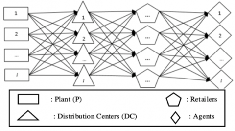
The distribution process from the production plant to consumers must go through several local distributors in several areas (multi-level) such as distributor centers, retailers, and agents [1]. The number of possible distribution networks that are formed to obtain minimal costs is a problem that needs to be considered. Determining the distribution network will be more complex when a company produces more than one type of product (multi-product) [2-4].
Figure 1. Multi-level distribution model
Based on Figure 1, the multi-level distribution model has many possible solutions to form the right distribution network, characterized by minimal costs [5, 8]. To minimize distribution costs, it is necessary to formulate a mathematical formulation in several variables to search for minimal costs and several main constraints that will affect the distribution network [5].
The data in this study are obtained through an interview process at a rice seed company. The data is adjusted to the problems in this study so that the data used are data on the stock capacity of each product for each level, vehicle capacity, number of vehicles, vehicle fixed costs, and costs of several products for each level of a distributor [8]. So the distribution problem can be adequately solved, and it is necessary to form a mathematical formulation for both the objective function and the constraints that follow it. The first is to form a formulation to describe the objective function of the distribution, which is the most minimal cost, so that to search for costs, the function used is in Eq. (1) which consists of several variables.
$z=\sum_{i=0}^{I}\left[\sum_{j=0}^{J} \sum_{k=0}^{K j} \sum_{r=0}^{R} \sum_{p=0}^{P j}\left(\left(X_{i j k r p} C_{i j p}\right)+C f_{i j k r}\right) S t_{i j k r}\right]$ (1)
i $\in$ {1, 2,..., I} is the level of distribution delivery, j $\in$ {1, 2,..., J} is the distributor unit that acts as the sender while r {1, 2,..., R} as order. P $\in$ {1, 2,..., P} is the type of product ordered, and k $\in$ {1, 2,..., K} is the vehicle owned by the distributor unit sending j to distribute its products. Xijkrp represents the number of units of goods to be shipped, Cvbijp is a variable cost for each product, Cfijkr is the fixed cost of delivery, and Stijkr is the status that the distributor at level i is shipping or not with his k vehicles {0,1}. After knowing the mathematical formulation of the following distribution problem is to form a mathematical formulation for the constraints that must be met so that the resulting solution is minimal in cost and meets the existing constraints so that the distribution problem can be solved correctly.
The demand constraint function is related to the limit on the number of orders from the customer so that the number of goods ordered by the customer (Oirp) must be the same as the goods sent later to the customer. The constraint function for the number of orders is shown in Eq. (2).
$\sum_{j=0}^{J} \sum_{k=0}^{K j} \sum_{r=0}^{R} \sum_{p=0}^{P j} X_{i j k r p}=O r_{i r p}$ (2)
The function of the vehicle capacity constraint for each distributor unit is the capacity of the vehicle used. An item is sent to the customer or the level below then the goods will be transported by the vehicle. The problem is that the vehicle capacity of each sending distributor (Cpijp) has a capacity limit that should not be violated. The constraint function for vehicle capacity is shown in Eq. (3).
$\sum_{j=0}^{J} \sum_{k=0}^{K j} \sum_{r=0}^{R} \sum_{p=0}^{P j} X_{i j k r p} \leq C p_{i j p}$ (3)
The inventory constraint function for each product at the distributor unit (Kcpijkp). Each distribution always has stock availability of goods. When a distributor acts as a sender, a stock check is carried out, the number of goods to be sent must not exceed the stock. The constraint function for the distribution unit stock of the sender is shown in Eq. (4).
$\sum_{j=0}^{J} \sum_{k=0}^{K j} \sum_{r=0}^{R} \sum_{p=0}^{P j} X_{i j k r p} \leq K c p_{i j k p}$ (4)
The search for solutions in distant neighbors is defined as a search with a random system so that it can reach a wide range of problems. After randomization and finding a solution in a specific area, it is continually searching for close neighbors, which is commonly known as a local search [11]. With this local search, the most superior solution will be found with VNS's ability to find the solution, so it is not trapped in a local optimum solution and can achieve a global optimum solution which is its advantage [12]. This algorithm is considered because it has been applied to solve transportation problems [13].
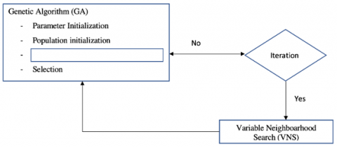
GA is a method that adopts individual biological traits in natural selection [14]. There are several steps in solving problems using GA, namely starting from chromosomal representation, reproduction, evaluation, and selection. The evaluation process in GA is used to measure how well an individual can provide a solution by considering the fitness value. The higher the fitness value produced by an individual in the next generation, the higher the probability of being selected as a solution [15]. Pseudocode hybrid GA-VNS is show in Figure 2. The GA-VNS hybridization process begins by running the GA algorithm until a certain iteration and then running the VNS algorithm to obtain the optimal fitness value. The GA-VNS hybridization architecture is shown in Figure 3.
Figure 2. Pseudocode VNS algorithm
Figure 3. GA-VNS hybridization architecture
The proportion of genetic algorithm hybridization is done with a percentage of 50 percent of iterations. The hybridization scenario of genetic algorithms and VNS to improve reproductive outcomes was carried out in the mid to late generation.
4.1 Chromosome representation and population initialization
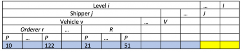
Chromosome representation is a process for modeling the solution of a problem. Chromosome representation is the initial and most important process to provide a solution to a problem. There are various kinds of coding in genetic algorithms, in this study using real-coded. The structure of the chromosomes in the genetic algorithm has a solution structure, as shown in Figure 4.
Figure 4. GA-VNS hybridization architecture
Each column contained in the solution represents the number of units of goods that will be sent to the ordering distributor. Each chromosome is also divided into segments. The number of segments depends on the number of levels required based on the order. Each segment has several subsegments. A subsegment of the "i" level segment is the sending distributor unit "j". The sending distributor sub-segment has a vehicle sub-segment that is used to make deliveries. Vehicle sub-segment is a distributor unit that places an order. The type of product ordered "p" becomes a sub-segment of the ordering distributor
4.2 Fitness function
A chromosome in the genetic algorithm has a function value used to measure the quality of the resulting solution. The function used is the fitness function. In the selection process, the fitness value is used to determine the selected chromosome. The greater the fitness value on the chromosome, the more likely it is to be selected as a solution. In this study, the fitness function is used to obtain the minimum distribution cost value. The formula used to find the fitness value is shown in Eq. (5).
fitness $=\frac{1}{Z}$ (5)
Z is the distribution cost shown in Eq. (1) which is owned by each chromosome.
4.3 Reproduction
The reproduction stage is a unique process owned by genetic algorithms to produce new individuals. Each new individual represents the solution to a problem. The reproduction process has two operators, namely crossover and mutation, which aim to explore further and deeper to find new individuals. Both operators aim to find new individuals who are better at solving problems [16]. There is a crossover rate (cr), and in the mutation operator, there is a mutation rate (Mr). The crossover rate and mutation rate function determine the number of new individuals produced in each process in one generation.
4.4 Crossover
One of the operators forming new individuals in the reproduction process is crossover. Crossover forms a new individual from two parents. The results obtained will vary because it inherits the properties of its two parents. The number of new individuals is obtained by multiplying the population size (Pop size) and the crossover rate (Cr). The crossover operator has various models that can be used, including one-cut-point, two-cut-point, and extended intermediate.
4.4.1 One-cut-point crossover
One-cut-point is a crossover model with one cut-off point for each gen. The mechanism is to cut the position of the gen in the two-parent individuals that have been randomly selected. Each parent was crossed until the cutting point between the first parent and the second parent [17]. An illustration of the crossover process with a one-cut-point model is shown in Figure 5.
Figure 5. One-cut-point crossover Mechanism
where, {x1, ..., } and yε{y1, ..., yn} are two randomly selected parent individuals and {z1, ..., } is the result of a crossover process called a new individual / child.
4.4.2 Two-cut-point crossover
Two-cut-point is developing the one-cut-point model that applies a cut point at two random gene positions on the chromosome. The new individual in this model results from the exchange of gene values between the two selected positions to the second individual [17]. An overview of the two-cut-point model at the second and sixth gene positions is illustrated in Figure 6.
Figure 6. Two-cut-point crossover mechanism
4.4.3 Extended intermediate
Extended intermediate crossover is a model that aims to change gene values based on a random number "α" with the difference in gene values in both individuals [18]. Eq. (6) is the result search function with an extended intermediate model.
$Z_{i}=x_{i}+a\left(y_{i}-x_{i}\right)$ (6)
4.5 Mutation
The second operator in the reproduction process that characterizes the genetic algorithm is mutation. Unlike the crossover operator, which must use two parents, the mutation operator only uses one parent to generate new individuals. The number of new individuals resulting from the multiplication of population size (pop size) and mutation rate (Mr). The mutation operator has several models, including: swap, insertion and simple random.
4.5.1 Swap
One of the mutation operator models is swap. This mutation operator model is to exchange values between two randomly selected gene positions [19].
4.5.2 Insertion
The insertion model is inserting the value of a particular position gene into another gene position. Gene values are generated randomly. The genes included in the insertion range will be shifted until they occupy the correct position with the number of genes [19, 20].
4.5.3 Simple random
Simple random is a mutation operator model that generates a random number (r) to increase or decrease the value of each gene after being added to 1. Variable Range (r) has a value of -0.1 to 0.1. Eq. (7) is a mathematical formulation on simple random mutation.
$x_{i}=x_{i}(1+r) \quad i=1, \ldots, n$ (7)
The reproductive process will be decided whether it needs to be repaired. If the reproduction results still reach the optimum local value, it will proceed to the hybridization process using variable neighborhood search (VNS). The hybridization process is carried out based on the generation parameters. In this mechanism, the percentage of hybridization is 50%. The hybridization process is carried out when the number of generations reaches half of the generations. For example, if the initially declared generation is 1000, then hybridization to improve reproduction results starts from the 500th generation. This reproduction will enter the selection process.
4.6 Selection
The selection process is to choose several chromosomes of population size (pop size) that will survive to become a new population in the following generation process based on the fitness value obtained. Several types of selection models in genetic algorithms, such as the roulette wheel, consider the cumulative probability of each individual's fitness value and elitism used in solving multi-level distribution problems [8]. The elitism selection model is to sort in descending order. In addition to the roulette wheel and elitism, there is also a binary tournament selection model. The binary tournament selection model compares the fitness value between two randomly selected individuals, and the individual with the most excellent fitness will be selected in the new population in the next generation.
At this stage, several tests were carried out to find the optimal genetic algorithm parameter values. Parameter testing carried out includes pop size, number of generations, Cr, and Mr. Each test scenario was carried out ten times and took the best fitness average value obtained. The next test is testing the best genetic operator model for optimizing the distribution of rice seeds. After testing the parameters and testing the reproductive operator model, an analysis is carried out on how well the model proposed in this study solves the problem of optimizing the distribution of rice seeds.
5.1 Parameter testing on GA
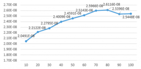
The application of multi-population in offering various solutions makes genetic algorithms able to solve optimization problems in several fields. Population size testing aims to determine the right population size in offering solutions so as to get optimal results. Figure 7 is the result of the population size test. The parameters used are the number of generations of 300, the value of Cr 0.5, and Mr 0.5. This combination of parameter values was chosen because it has been tested in previous distribution studies, and the crossover, mutation, and selection models were used [8].
Figure 7. Population size tests
The determination of the pop size is seen from the starting point of the convergence condition based on the graph of the average fitness value in Figure 6. Convergent conditions are conditions when on a more extensive test, the results shown have relatively minor differences so that Based on Figure 7, pop size 60 is the starting point for convergence.
At the pop size value below 60, the average fitness results on the graph show a significant increase in results. The smaller the pop size value means fewer solutions are offered, making it challenging to find the optimal solution. While the pop size value is more than 60, the average fitness result also increases to 80, although the difference is not significant. When the pop size value is more than 90, there is a decrease in the results, which indicates the optimal solution has been obtained. If the popo size test is continued, the results obtained will not be better. When the pop size value of 90 and 100, the fitness value decreased, but the decrease would not differ much from the selected pop size result of 60.
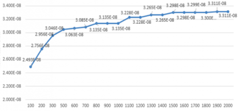
5.2 Generations testing
Determination of the optimal number of generations is chosen from the point of convergence. Convergence is a condition when the solutions offered have insignificant differences. Figure 7 results from testing the number of generations with the best population size from the previous test, 60. The combination of cr and Mr used is still the same as the previous test.
The test of the number of generations in Figure 8 shows that the best average of each experiment is unstable due to the high level of problem complexity. Based on the best fitness value, the fitness convergence point is at the 1100th generation. This point was chosen because the change in the best fitness value in the larger generation did not have a significant difference.
Figure 8. Results number of generations testings
5.3 Combination of crossover rate (Cr) and Mutation Rate (Mr)
Parameter testing of the combination of Cr and Mr values was carried out to maintain the diversity of the solutions produced by the reproduction process. Figure 8 is the average fitness value of the test results for the Cr and Mr values with the pop size value and the number of generations of previous test results.
Figure 9. Fitness value of the test results for the Cr and Mr
The test results in Figure 9 show that the values of Cr 0.8 and Mr 0.2 are the right combinations for multi-level multi-product distribution problems. In this combination, the resulting solution shows the best results with more individual diversity from the mutation process.
5.4 Crossover model testing
Table 1. Crossover model results
|
No |
Crossover Model |
Average Fitness |
Average Costs |
|
1 |
Crossover One-Cut-Point |
2.54088E-8 |
39583805 |
|
2 |
Crossover Two-Cut-Point |
3.07092E-8 |
32679440 |
|
3 |
Crossover Extended Intermediate |
2.49052E-8 |
40537165 |
In this test, the three crossover models will be compared, namely: one-cut-point, two-cut-point, and extended intermediate. Table 1 is the testing process carried out using the genetic algorithm parameters selected from the previous test results, namely population size 80, number of generations 800, Cr 0.3, and Mr 0.7. Based on the testing of the crossover model in Table 1, it can be concluded that the best crossover model is a two-cut point. The two-cut point model obtains the most extensive average fitness.
Mutation model test results done by comparing swap, insertion, and simple random. Based on the average fitness and the resulting average cost, swap mutation provides a better solution than other methods. The results of testing the mutation model can be seen in Table 2.
Table 2. Mutation model results
|
No |
Model Selection |
Average Fitness |
Average Costs |
|
1 |
Swap Mutation |
3.18331E-8 |
31484625 |
|
2 |
Insertion Mutation |
2.83421E-8 |
35348305 |
|
3 |
Simple Random Mutation |
2.36457E-8 |
42419490 |
5.5 Selection model testings
Selection model testing aims to find the selection model that produces the best fitness value. Three selection models will be compared in this test, namely elitism, roulette wheel, and binary tournament. Table 3 is the result of the average fitness with the cost of each model. Based on the test results, the elitism selection model gets the best average fitness value and the most negligible distribution cost.
Table 3. Selection model results
|
No |
Model Selection |
Average Fitness |
Average Costs |
|
1 |
Elitism Selection |
3.13905E-8 |
31994380 |
|
2 |
Roulette-wheel Selection |
1.15668E-8 |
86463140 |
|
3 |
Binary Tournament Selection |
2.81680E-8 |
94982361 |
The next stage is to test the quality of the proposed GA-VNS algorithm. In this test, a combination of optimal parameter values is used based on the results of previous tests. A comparison was made of three algorithms: random search (RS), genetic algorithm (GA), and GA-VNS hybridization.
Table 4. Overall algorithm results
|
No |
Algorithm |
Average Fitness |
Average Costs |
|
1 |
RS |
2.05077E-8 |
48784775 |
|
2 |
GA |
3.06647E-8 |
32716150 |
|
3 |
GA-VNS |
3.09724E-8 |
32392960 |
Based on the test results in Table 4. each algorithm obtains a different average computation time. The random search algorithm takes the fastest time based on the computational time, but the resulting fitness results are still low. The time required for the GA and hybrid GA-VNS algorithms is relatively the same, but the hybrid GA-VNS algorithm provides the best average fitness results and minimal distribution costs.
The multi-level and multi-product distribution problem in this research is solved by forming a mathematical model of several variables whose goal is to get the minimum cost. The variables used are the number of products, variable costs, vehicles used, fixed costs, and delivery status. The variables used to resolve some of the constraints that occur in the distribution process, such as the number of products distributed, must be the same as the number of orders and do not exceed the vehicle's maximum capacity or the amount of stock owned.
Based on the mathematical model compiled, the solution to the problem of rice seed distribution consists of a series of genes. Each gene of the chromosome contains an actual number indicating the number of products to be distributed. The best solution is selected based on the resulting fitness value. The greater the fitness value indicates the minimal cost of the distribution process.
Based on the test results of several selection models, the elitism model obtains the best fitness value. Based on testing the parameter values and the production operator model on the GA-VNS algorithm, the GA-VNS algorithm provides a solution with near-optimal results with relatively the same computational time compared to the GA algorithm, namely 279332 ms and 265091 ms. The fitness results obtained from the GA-VNS algorithm are also better, namely 32392960 and the classic GA, which is 32716150. The fitness results generated by the GA-VNS algorithm provide the most minimal cost with a savings of 16391815.8.
The authors would like to thank the University of Jember and Airlangga University for their assistance in carrying out this research. This work is supported by Islamic Development Bank (IDB).
[1] Guo, H., Wang, X., Zhou, S. (2015). A transportation problem with uncertain costs and random supplies. International Journal of E-Navigation and Maritime Economy, 2: 1-11. https://doi.org/10.1016/j.enavi.2015.06.001
[2] Gicquel, C., Minoux, M. (2015). Multi-product valid inequalities for the discrete lot- sizing and scheduling problem. Computers and Operation Research, 54: 12-20. http://dx.doi.org/10.1016/j.cor.2014.08.022
[3] Kim, S.H., Lee, Y.H. (2016). Synchronized production planning and scheduling in semiconductor fabrication. Computers & Industrial Engineering, 96: 72-85. http://dx.doi.org/10.1016/j.cie.2016.03.019
[4] Langroodi, R.R.P., Amiri, M. (2016). A system dynamics modeling approach for a multi-level, multi-product, multi-region supply chain under demand uncertainty. Expert Systems with Applications, 51: 231-244. http://dx.doi.org/10.1016/j.eswa.2015.12.043
[5] Sitek, P., Wikarek, J. (2012). Mathematical programming model of cost optimization for supply chain from perspective of logistics provider. Management and Production Engineering Review, 3: 49-61.
[6] Gupta, A., Narayan, V., Raj, A., Nagaraju, D. (2012). A comparative study of three echelon inventory optimization using genetic algorithm and particle swarm optimization. International Journal of Trade, Economics and Finance, 3(3): 205-208.
[7] Chen, Z.Q., Wang, R.L. (2011). Solving the m‐way graph partitioning problem using a genetic algorithm. IEEJ Transactions on Electrical and Electronic Engineering, 6(5): 483-489. https://doi.org/10.1002/tee.20685
[8] Sarwani, M.Z., Rahmi, A., Mahmudy, W.F. (2017). An adaptive genetic algorithm for cost optimization of multi-stage supply chain. Journal of Telecommunication, Electronic and Computer Engineering (JTEC), 9(2-7): 155-160.
[9] Behera, S.K., Parhi, D.R., Das, H.C. (2018). A hybrid intelligent model for crack diagnosis in a free-free aluminium beam structure. Modelling, Measurement and Control B, 87(2): 68-77. https://doi.org/10.18280/mmc_b.870202
[10] Zhu, Y.X., Wang, J.J., Li, M.Y. (2020). Collaborative distribution in the soft time window of agricultural-means supply chain based on simulated annealing-genetic algorithm. Journal Européen des Systèmes Automatisés, 53(6): 835-844. https://doi.org/10.18280/jesa.530609
[11] Cheikh, M., Ratli, M., Mkaouar, O., Jarboui, B. (2015). A variable neighborhood search algorithm for the vehicle routing problem with multiple trips. Electronic Notes in Discrete Mathematics, 47: 277-284. http://dx.doi.org/10.1016/j.endm.2014.11.036
[12] Castelli, M., Vanneschi, L. (2014). Genetic algorithm with variable neighborhood search for the optimal allocation of goods in shop shelves. Operations Research Letters, 42(5): 355-360. http://dx.doi.org/10.1016/j.orl.2014.06.002
[13] Ziebuhr, M., Kopfer, H. (2016). Solving an integrated operational transportation planning problem with forwarding limitations. Transportation Research Part E: Logistics and Transportation Review, 87: 149-166. http://dx.doi.org/10.1016/j.tre.2016.01.006
[14] Qiongbing, Z., Lixin, D. (2016). A new crossover mechanism for genetic algorithms with variable-length chromosomes for path optimization problems. Expert Systems with Applications, 60: 183-189. http://dx.doi.org/10.1016/j.eswa.2016.04.005
[15] Thakur, M., Kumar, A. (2016). Optimal coordination of directional over current relays using a modified real coded genetic algorithm: A comparative study. International Journal of Electrical Power & Energy Systems, 82: 484-495. http://dx.doi.org/10.1016/j.ijepes.2016.03.036
[16] Jiao, R., Yang, Z., Shi, R., Lin, B. (2014). A multistage multiobjective substation siting and sizing model based on operator–repair genetic algorithm. IEEJ Transactions on Electrical and Electronic Engineering, 9(S1): S28-S36. https://doi.org/10.1002/tee.22042
[17] Arora, J.S., Arora, J.S. (2012). Chapter 16 – Genetic Algorithms for Optimum Design, Elsevier Inc.
[18] Mahmudy, W.F. (2015). Optimization of part type selection and machine loading problems in flexible manufacturing system using variable neighborhood search. IAENG Int. J. Comput. Sci, 42(3): 254-264.
[19] Soni, N., Kumar, T. (2014). Study of various mutation operators in genetic algorithms. International Journal of Computer Science and Information Technologies, 5(3): 4519-4521.
[20] Mladenovic, N., Urosevic, D., Perez-Brit, D. (2016). Variable neighborhood search for minimum linear arrangement problem. Yugoslav Journal of Operations Research, 26(1): 3-16. https://doi.org/10.2298/YJOR140928038M