Meshal Harbi Odah
© 2021 IIETA. This article is published by IIETA and is licensed under the CC BY 4.0 license (http://creativecommons.org/licenses/by/4.0/).
OPEN ACCESS
Financial time series are defined by their fluctuations, which are characterized by instability or uncertainty, implying that there are periods of volatility followed by periods of relative calm. Therefore, time series analysis requires homogeneity of variance. In this paper, some models used in time series analysis have been studied and applied. Comparison between Autoregressive Moving Average (ARMA) and Generalized Autoregressive Conditionally Heteroscedastic (GARCH) models to identify the efficient model through (MAE, MASE) measures to determine the best forecasting model is studied. The findings show that the models of Generalised Autoregressive Conditional Heteroscedastic are more efficient in forecasting time series of financial. In addition, the GARCH model (1,1) is the best to forecasting exchange rate.
GARCH, ARMA, financial time series, heteroskedasticity
Interest in using time-series models has grown widely in many areas, the most important of which is the economic field, in particular, the financial data. Recent years witnessed rapid development in the study of financial time series, which are characterized by instability or uncertainty. In this respect, there are periods of volatility followed by periods of relative calm, which necessitates the use of analytical models that can be formulated for those periods with mathematical models that allow for future planning and correct decision-making.
To achieve high-efficiency results, the process of predicting the future behavior of the studied phenomenon is important in many fields such as commercial, industrial, and government. There are several studies investigating Forecasting in the previous literature forecasting models have been employed.
For example, Odah [1] used the Autoregressive Integrated Moving Average model (ARIMA) method to model the prediction of the urban population growth rate. Various approaches were applied by Sun et al. [2] to model solar radiation series with ARMA–GARCH models in climate stations/ China. The authors claimed that the ARMA–GARCH(-M) models were the best method for modeling solar radiation series. Mohammed [3] employed ARCH, GARCH models in prediction at the daily closing price for the Iraqi stock exchange index. The study uncovered the accuracy of forecasting was depend on forecasting accuracy criterion. Similarly, Liu and Shi [4] used ARMA–GARCH approaches to forecast short-term electricity prices. The results demonstrated that the employed model was a useful tool for modeling and forecasting the mean and volatility of electricity prices.
Ghani and Rahim [5] conducted research to present the best ARMA-GARCH model using various specification formats. In their emphasis, they used the Generalized Autoregressive Conditional Heteroscedasticity (GARCH) model. They argued that the ARMA-GARCH model is superior to others in terms of volatility modeling. Goh et al. [6] investigated the characteristics of price volatility in the Malaysian market using ARCH-type models and Rubber Grade 20 (SMR 20). The authors have claimed that the FIGARCH model is the best for both short- and long-term forecasting. In another respect, Rahmadayanti et al. [7] employed Autoregressive (AR) and Generalized Autoregressive Conditional Heteroskedasticity (GARCH) models to calculate VaR for two stock indexes with normal distributions. According to the study, the GARCH model with a normal distribution has better performance with a total error rate of 26. In order to examine the behavior of the exchange rate in Tanzania, Epaphra [8] employed univariate nonlinear time series analysis of the daily exchange rate data. According to the findings of the study, the GARCH model can accurately model the volatility of currency rates. El Jebari and Hakmaoui [9] carried out a comparison study of univariate nonlinear time series analysis of daily exchange rate data to investigate the behavior of Tanzania's exchange rate. According to the findings of the study, the GARCH model can accurately model the volatility of currency rates. In another respect and using various GARCH-class models, Ulussever et al. [10] carried out an estimation study to investigate electricity market volatility in Turkey.
According to the above Previous literature did not compare autoregressive moving average (ARMA) and conditional autoregressive models (GARCH) for exchange rate forecasting during past periods, many models were used to predict the exchange rate, and due to its importance being one of the factors affecting economic growth, it is difficult to forecast the realistic exchange rate. On the other hand, as it is known that forecasting financial time series is a complex process because it is a non-stationary time series and is characterized by volatility, it is necessary to choose forecasting models to be applicable in the Iraqi market, especially after the Central Bank of Iraq’s decision to raise the exchange rate at the end of 2020.
The aim of this paper is to compare the Autoregressive Moving Average (ARMA) and Generalized Autoregressive Conditionally Heteroscedastic (GARCH) models to identify the most efficient model through (MAE, MASE) measures that can predict the exchange rate.
Forecasting the fluctuations of time series of financial variables is of particular importance due to its impact on decision-making and with regard to the exchange rate in particular, it is one of the important variables affecting the management of macroeconomic policy, especially monetary policy the past. In this paper, Autoregressive Moving Average (ARMA) models are employed to forecast the exchange rate this methodology is based on a consolidating between autoregressive model and the moving average model, Generalized Autoregressive Conditional Heteroscedasticity (GARCH) models are applied when the data is characterized by uncertainty and heterogeneity. In the following subsections, the ARMA and GARCH models are described.
2.1 ARMA models
The AR (p) model is expressed as follows:
$y_{t}=\alpha+\delta_{1} y_{t-1}+\delta_{2} y_{t-2}+\cdots+\delta_{p} y_{t-p}+\varepsilon_{t}$ (1)
$y_{t}=\alpha+\sum_{i=1}^{p} \delta_{i} y_{t-i}+\varepsilon_{t}$ (2)
where, yt is the actual value at current period t, εt random error at current period t, δi (i=1, 2..., p) are the model parameters and α is a constant. Then, the MA (q) is expressed as follows:
$y_{t}=\alpha+\eta_{1} \varepsilon_{t-1}+\eta_{2} \varepsilon_{t-2}+\cdots+\eta_{q} \varepsilon_{t-q}+\varepsilon_{t}$ (3)
$y_{t}=\alpha+\sum_{i=1}^{q} \eta_{i} \varepsilon_{t-i}+\varepsilon_{t}$ (4)
where, α is a constant and (ηi, i=1, 2..., q) are the model parameters and q is the order of the model. Shumway and Stoffer [11] showed that the combination of (AR (P), MA (q)) processes is the mixed autoregressive – moving average process. Therefore, ARMA (p, q) can be formulated as follows:
$\begin{aligned} \mathrm{y}_{\mathrm{t}}=\alpha+\delta_{1} \mathrm{y}_{\mathrm{t}-1} &+\delta_{2} \mathrm{y}_{\mathrm{t}-2}+\cdots+\delta_{\mathrm{p}} \mathrm{y}_{\mathrm{t}-\mathrm{p}}+\varepsilon_{\mathrm{t}} -\eta_{1} \varepsilon_{\mathrm{t}-1}-\eta_{2} \varepsilon_{\mathrm{t}-2}-\cdots-\eta_{\mathrm{q}} \varepsilon_{\mathrm{t}-\mathrm{q}} \end{aligned}$ (5)
$\mathrm{y}_{\mathrm{t}}=\alpha+\sum_{\mathrm{i}=1}^{\mathrm{p}} \delta_{\mathrm{i}} \mathrm{y}_{\mathrm{t}-\mathrm{i}}+\varepsilon_{\mathrm{t}}-\sum_{\mathrm{i}=1}^{\mathrm{q}} \eta_{\mathrm{j}} \varepsilon_{\mathrm{t}-\mathrm{j}}$ (6)
2.2 GARCH models
The ARCH models are statistical techniques are used to study and forecast the conditional variances [12]. According to these models, the variance of the time series is not constant and can be expressed as:
$\sigma_{t}^{2}=\alpha+\theta_{1} \varepsilon_{t-1}^{2}+\theta_{2} \varepsilon_{t-2}^{2}+\cdots+\theta_{q} \varepsilon_{t-q}^{2}$ (7)
$\sigma_{t}^{2}=\alpha+\sum_{i=1}^{q} \theta_{i} \varepsilon_{t-i}^{2}$ (8)
where, $\sigma_{t}^{2}$ conditional variance of random error εt and θ is the parameter of the model. Generalized Autoregressive Conditional Heteroscedastic models seek to simulate the path of financial time series by via statistical processing of the proposed model from by Bollerslev [13]. It is defined as an equation of volatility and can be shown as:
$\sigma_{t}^{2}=\alpha+\theta_{1} \varepsilon_{t-1}^{2}+\theta_{2} \varepsilon_{t-2}^{2}+\cdots+\theta_{q} \varepsilon_{t-q}^{2}+\beta_{1} \sigma_{t-1}^{2}$$+\beta_{2} \sigma_{t-2}^{2}+\cdots+\beta_{p} \sigma_{t-p}^{2}$ (9)
$\sigma_{t}^{2}=\alpha+\sum_{i=1}^{q} \theta_{i} \varepsilon_{t-i}^{2}+\sum_{j=1}^{p} \beta_{j} \sigma_{t-j}^{2}$ (10)
The best model for forecasting financial time series will be applied in the fourth section through several steps, including identification, parameters estimation, model diagnostic, and forecasting.
The best model will be determined by the smaller the forecast error. By applying the standards below:
3.1 Mean Absolute Error (MAE)
We will use a standard mean absolute error (MAE) is in assessing average model performance and can be expressed as [14]:
$\mathrm{MAE}=\frac{1}{n} \sum_{i=1}^{n}\left|f_{i}-y_{i}\right|=\frac{1}{n}\left|\varepsilon_{i}\right|$ (11)
3.2 Mean Absolute Scaled Error Measurement (MASE)
We will use a standard Mean Absolute Scaled Error (MASE) is determine the criterion of the accuracy of forecasts and can be expressed as [15]:
MASE $=\frac{1}{n} \sum_{i=1}^{n}\left(\frac{\left|\varepsilon_{t}\right|}{\frac{1}{n-1} \sum_{i=2}^{n}\left|y_{i}-y_{i-1}\right|}\right)=\frac{\sum_{t-1}^{n}\left|\varepsilon_{t}\right|}{\frac{n}{n-1} \sum_{i=2}^{n}\left|y_{i}-y_{i-1}\right|}$ (12)
Data on the exchange rate of the Iraqi dinar against the USD was collected daily, except for non-trading days. The data was the rate of (1490) observed by the Central Bank of Iraq for the period from 4.1.2015 to 17.3.2021. This period was chosen due to the economic instability of the cohttps://www.iieta.org/node/10299/edituntry.
Figure 1. The plot of time series for the exchange rate of the Iraqi dinar against USD ($) for the period (4.1.2015 to 17.3.2021) (S1)
Figure 1 shows that the exchange rate time series is unstable and has high volatility, which indicates the presence of variability in variability. The reason for this is that the Central Bank of Iraq raised the exchange rate, which led to market instability. We note from the Figure 1 that the exchange rate increased in the last months of the years 2020 and 2021.
4.1 Time series stability tests
The time series stability tests unity root s is examined using KPSS and Philips-Perron tests for time series data to detect the unstable String data as shown in Table 1 (S1).
Table 1. The outcomes of the tests for the time series (S1)
|
Model test |
Intercept |
Trend & Intercept |
None |
|
ADF |
-0.538 |
-0.217 |
-0.507 |
|
Philips-Perron |
-0.624 |
-0.295 |
-0.497 |
|
KPSS |
0.976 |
0.809 |
|
Table 2 shows the outcomes of the model tests after taking the first-order difference the results indicate the time series does not include a unit root after taking the first difference for series (∆S1).
Table 2. The outcomes of the model tests after taking the first-order difference (∆S1)
|
Model test |
Intercept |
Trend & Intercept |
None |
|
ADF |
-34.048 |
-34.158 |
-34.058 |
|
Philips- Perron |
-34.337 |
-34.359 |
-34.346 |
|
KPSS |
0.634 |
0.160 |
|
The Figure 2 shows the stability of the exchange rate series after taking the first difference of the data, which means that there is no false forecasting to the instability of the time series.
Figure 2. The plot of time series for exchange rate after taken the first-order difference (∆S1)
Figure 3. The Descriptive statistics and basic tests for time series data after taken the first-order difference (∆S1)
According to Figure 3, the value of the skewness coefficient was (6.882443), which indicates that the error distribution is skewed to the right (positive skewed). Furthermore, the kurtosis coefficient value is (196.5858), indicating that the time series (EX) is dispersed and thus deviates from the normal distribution. Result is shown by the Jarque-Bera statistics, which indicate the exchange rate time series does not follow the normal distribution at a significant level (0.05).
4.2 Model analysis
The results of the analysis models are compared to ARAM and GARCH in this section using forecasting accuracy, Test Mean Absolute Error, and Mean Absolute Scaled Error. The following measurements are shown in the Tables 3, 4, 5 and 6.
Based on an examination of Table ARAM, we identified the model (2, 2) that provided the best representation of the time series of the exchange rate, as shown in Table 3.
Table 3. The results of estimating tests ARAM models
|
ARAM |
||||
|
Variable |
Coefficient |
Std. Error |
t-Statistic |
Prob. |
|
C |
0.162283 |
0.176855 |
0.917603 |
0.3590 |
|
AR (1) |
-1.206784 |
0.066254 |
-18.21464 |
0.0000 |
|
AR (2) |
-0.498167 |
0.080795 |
-6.165821 |
0.0000 |
|
MA (1) |
1.305468 |
0.067093 |
19.45773 |
0.0000 |
|
MA (2) |
0.634162 |
0.080006 |
7.926427 |
0.0000 |
|
Akaike |
6.230145 |
|||
|
Schwarz |
6.251525 |
|||
|
Hannan-Quinn |
6.238113 |
|||
|
Durbin-Watson |
2.011268 |
|||
It was an ARCH test effect is clear in the residues series, which necessitated us to analyze the series with GARCH models this is a general feature of the time series of financial.
Table 4. The results of the ARCH test for the time series
|
Heteroskedasticity Test: ARCH MODEL |
|||
|
F-statistic |
20.60731 |
Prob.F(1,1486) |
0.0000 |
|
Obs*R-squared |
20.35280 |
Prob.Chi-Square (1) |
0.0000 |
Via Table 4, results of the table show out that the value Obs*R-squared=20.35280 value Prob Chi-Square (1) less than 0.05. This indicates that the error variance is not constant over time, meaning that the residuals are influenced by the ARCH model.
Table 5. The forecasting accuracy test for GARCH and ARMA models
|
|
GARCH (1,1) |
ARAM (2,2) |
|
MAE |
0.003158 |
0.002856 |
|
MASE |
0.006345 |
0.006561 |
Table 5 assesses the validity of forecasting the exchange rate through the study models. The MAE, MASE is compared with each other for estimated models where the GARCH model (1,1) the best to forecasting exchange rate.
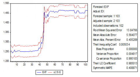
According to Figure 4, the forecasting of the exchange rate within the sample for the last three months, using a model, GARCH (1, 1) for forecasting, shows that the exchange rate of the Iraqi dinar against the US dollar will rise in the coming days, indicating an increase in the goods and services provided.
Table 6. The estimating GARCH model for the time series
|
GARCH (1,1) |
||||
|
Variable |
Coefficient |
Std. Error |
Z-Statistic |
Prob |
|
C |
0.0158821 |
1.756928 |
9.247501 |
0.0000 |
|
Variance Equation |
||||
|
ARCH (1) |
0.052401 |
0.007066 |
10.69343 |
0.0000 |
|
GARCH (1) |
0.924291 |
0.002311 |
154.7974 |
0.0000 |
|
Akaike |
5.262808 |
|||
|
Schwarz |
5.280625 |
|||
|
Hannan- Quinn |
5.269448 |
|||
|
Durbin- Watson |
1.839777 |
|||
Figure 4. Forecasting exchange rate for last three months within the sample
In this paper, time series analysis requires homogeneity of variance. Some models used in time series analysis have been studied and applied. Comparison between Autoregressive Moving Average (ARMA) and Generalized Autoregressive Conditionally Heteroscedastic (GARCH) models to identify the efficient model.
The results showed that the financial chain of the exchange rate is characterized by an unstable series after performing unit root tests, taken the first-order difference for the string to be stable the study also showed that forecasting the exchange rate through the study models, the MAE, MASE is compared with each other for estimated models where GARCH model (1,1) the best to forecasting exchange rate, from the Figure 4 for forecast it shows the rise in the exchange rate of the Iraqi dinar against the US dollar for the coming days, which indicates an increase in the goods and services provided. Finally, the models of Generalised Autoregressive Conditional Heteroscedastic are more efficient in forecasting time series of financial.
|
ARMA |
Autoregressive Moving Average |
|
GARCH |
Generalized Autoregressive Conditionally Heteroscedastic |
|
MAE |
Mean Absolute Error |
|
MASE |
Mean Absolute Scaled Error Measurement |
|
AR |
Autoregressive |
|
MA |
Moving Average |
|
ARCH |
Autoregressive Conditional Heteroskedasticity |
|
EX |
Exchange rate |
|
EX1 |
Exchange rate after taken the first-order difference |
|
S1 |
Time Series |
[1] Odah, M.H. (2020). Comparison of Box-Jenkins models predicting Iraq’s population growth rate. In IOP Conference Series: Materials Science and Engineering, 928(4): 042045. https://doi.org/10.1088/1757-899X/928/4/042045
[2] Sun, H., Yan, D., Zhao, N., Zhou, J. (2015). Empirical investigation on modeling solar radiation series with ARMA–GARCH models. Energy Conversion and Management, 92: 385-395. https://doi.org/10.1016/j.enconman.2014.12.072
[3] Mohammed, M.A. (2015). Using ARCH, GARCH models in prediction at daily closing price for Iraqi stock exchange index. Journal of Kirkuk University for Administrative and Economic Sciences, 5(2): 237-266. https://www.iasj.net/iasj/article/106691
[4] Liu, H., Shi, J. (2013). Applying ARMA–GARCH approaches to forecasting short-term electricity prices. Energy Economics, 37: 152-166. https://doi.org/10.1016/j.eneco.2013.02.006
[5] Ghani, I.M., Rahim, H.A. (2019). Modeling and forecasting of volatility using ARMA-GARCH: Case study on Malaysia natural rubber prices. In IOP Conference Series: Materials Science and Engineering, 548(1): 012023. https://doi.org/10.1088/1757-899X/548/1/012023
[6] Goh, H.H., Tan, K.L., Khor, C.Y., Ng, S.L. (2016). Volatility and market risk of rubber price in Malaysia: Pre-and Post-global financial crisis. Journal of Quantitative Economics, 14(2): 323-344. https://doi.org/10.1007/s40953-016-0037-4
[7] Rahmadayanti, C., Umbara, R.F., Rohmawati, A.A. (2018). Prediksi value-at-risk dengan efek autoregressive conditional heteroskedasticity (ARCH). E-Proceedings of Engineering, 5(2): 3846.
[8] Epaphra, M. (2016). Modeling exchange rate volatility: Application of the GARCH and EGARCH models. Journal of Mathematical Finance, 7(1): 121-143. https://doi.org/10.4236/jmf.2017.71007
[9] El Jebari, O., Hakmaoui, A. (2018). Forecasting the volatility of the Moroccan financial market: A comparison between the models of GARCH family and EWMA. Journal of Insurance and Financial Management, 3(5): 1-17.
[10] Ulussever, T., Soytaş, M.A., Ertuğrul, H.M. (2017). Modelling price dynamics in Turkish electricity market: lessons from GARCH estimates. Marmara Üniversitesi İktisadi ve İdari Bilimler Dergisi, 39(2): 621-638. https://doi.org/10.14780/muiibd.384221
[11] Shumway, R.H., Stoffer, D.S. (2017). ARIMA models. In Time Series Analysis and Its Applications, pp. 75-163.
[12] Engle, R.F. (1982). Autoregressive conditional heteroscedasticity with estimates of the variance of United Kingdom inflation. Econometrica: Journal of the Econometric Society, 50(4): 987-1007. https://doi.org/10.2307/1912773
[13] Bollerslev, T. (1986). Generalized autoregressive conditional heteroskedasticity. Journal of Econometrics, 31(3): 307-327.
[14] Willmott, C.J., Matsuura, K. (2005). Advantages of the mean absolute error (MAE) over the root mean square error (RMSE) in assessing average model performance. Climate Research, 30(1): 79-82.
[15] Hyndman, R.J. (2006). Another look at forecast-accuracy metrics for intermittent demand. Foresight: The International Journal of Applied Forecasting, 4(4): 43-46.