Collins Olusola Akeremale* | Oluwasegun Adeyemi Olaiju | Su Hoe Yeak
© 2021 IIETA. This article is published by IIETA and is licensed under the CC BY 4.0 license (http://creativecommons.org/licenses/by/4.0/).
OPEN ACCESS
This article considered the traditional finite element method (FEM) and adaptive finite element method (FEM) for the numerical solution of the one-dimensional boundary value problems. We established the preference or the superiority of the h-adaptive FEM to traditional FEM in high gradient problems in terms of accuracy and cost of computation. Numerical examples which confirm the performance and adaptability of the h-adaptive method over the traditional finite element method and the high accuracy of the numerical solution are presented. Detailed error analysis of linear elements was also discussed. In conclusion, h-adaptive FEM is recommended for complex systems with high gradient problems.
adaptivity, advection, fine region, finite element method, high-gradient
Most natural phenomena are characterized by high gradients where a rapid change in the solution of the model occurs. Using global or uniform refinement may resolve the issue at a very high computational cost and time since these high gradients are normally localised [1, 2]. It is essential to accurately solve such models (problems) as it helps to make appropriate decisions and to predict future occurrences. Though there are different numerical methods for the solution of such models (differential equations) [3, 4] in this article, the finite element method is adopted because it is efficient, accurate, easy to code and able to handle irregular geometry [5]. The finite element method is one of the numerical approaches to boundary value problems. The method concerns partitioning the domain of the solution into a finite number of essential subdomains and using the variational approach to create an estimate of the solution over the set of finite elements. In general, the underlying idea of this method had been used with impressive accomplishment in solving problems, virtually in all fields of mathematical physics and engineering [6, 7].
The (FEM) has been used extensively to approximate the solution of partial differential equations [8, 9]. To give a smooth solution, the FEM has been improved upon in many ways. However, applications of this technique to high gradient boundary value problems are not trivial. For high gradients and singularities problems, mesh refinement is needed.
Moreover, for any discontinuous or high gradient problem, uniform refinement may be extremely expensive for these classes of problems. This is because many elements that are not in the high gradient region and do not require refinement will be refined thereby resulting in serious oscillation in the solution [10-12]. Thus, using local refinement that selectively refines only the elements within the high gradient region seems to be a better choice [13-16]. The adaptive finite element method [9, 17-19] has the potential to overcome this problem and produce accurate results without refining the mesh of the whole domain.
High gradients, as often found in engineering applications, such as fluid, turbulence, shocks, often affect the optimal performance, tolerance, and physical behaviour of such applications. Therefore, effective, and efficient advanced numerical methods in modelling such behaviours are essential in the scientific community [19, 20].
This article employs the adaptive FEM to approximate the high gradient problems to establish the superiority of the adaptive FEM over FEM. It was observed from the given examples in this work that adaptive finite element performs better in term accuracy and computational time compared to traditional finite element method. In section two, the methodology is discussed, section three discusses the results and finally, section four discusses the conclusion and recommendations. Figure 1 and Figure 2 below shows a linear adaptive geometry and geometry with six degrees of polynomial without adaptive respectively
Figure 1. A linear polynomial adaptive FE geometry for second elements (h-adaptive)
Figure 2. Galerkin FE with six degrees of polynomial interpolation in each element
Consider the general steady one-dimensional second-order ordinary differential advection-dominated equation with two boundary conditions below:
$D \frac{\partial^{2} u}{\partial x^{2}}-v \frac{\partial u}{\partial x}+c(x) u(x)=f(x), \quad 0<x<1$ (1)
where, v and D are the known constant velocity (advection) and diffusivity, respectively.
With the boundary conditions u(0)=u0, u(L)=un, where u is an unknown scalar function of x on the interval [xL, xR], f and c are given functions of x. The function f(x) is the known source function.
The finite element method (FEM) is a numerical approach for partial differential equations with boundary conditions. It subdivides the domain of the problem into simpler parts, called elements, and adopts a residual approach for the solution of the problem through minimization of the error function associated with the discretized problem [6, 7].
The main task in the finite element method is finding approximate solution u such that.
$u^{e}=\sum_{i=1}^{n} N_{i} u_{i}$
where, n is the total number of nodes in the domain and Ni is the basis function corresponding to the nodes in each element, as shown in Figure 3. A system of equations is generated and solved. The solution of FEM in its weak form is C0 continuous, and it includes boundary conditions in its formulation.
Eq. (1) is converted to weak form by integration over the domain as:
$\int_{\Omega}\left[D \frac{\partial^{2} u}{\partial x^{2}}-v \frac{\partial u}{\partial x}+c(x) u(x)\right] d x=\int_{\Omega}(w \cdot f) d x$ (2)
Eq. (2) becomes,
$\begin{aligned}\left.w \cdot D \frac{\partial u}{\partial x}\right|_{0} ^{L}-\int_{0}^{L} w & \cdot v \frac{\partial u}{\partial x} d x \\ &=\int_{0}^{L} w \cdot f d x-\int_{0}^{L} w \cdot c(x) u(x) d x \end{aligned}$ (3)
where, w is any weight function.
Let, w(0)=0, and $\frac{\partial u}{\partial x}=u_{n}$, we get from Eq. (3),
$w(L) \cdot D \cdot u_{n}-\int_{0}^{L} D \frac{\partial w}{\partial x} \frac{\partial u}{\partial x} d x-\int_{0}^{L} w \cdot v \frac{\partial u}{\partial x}$
$=\int_{0}^{L} w \cdot f d x-\int_{0}^{L} w \cdot c(x) u(x) d x$ (4)
$w(L) \cdot D \cdot u_{n}-\sum_{i=1}^{n-1} \int_{x_{i}}^{x_{i-1}} D \frac{\partial w}{\partial x} \frac{\partial u}{\partial x} d x$
$-\sum_{i=1}^{n-1} \int_{x_{i}}^{x_{i-1}} w \cdot v \frac{\partial w}{\partial x} d x$
$=\sum_{i=1}^{n-1} \int_{x_{i}}^{x_{i-1}} w \cdot f d x-\sum_{i=1}^{n-1} \int_{x_{i}}^{x_{i-1}} w \cdot c(x) u(x) d x$ (5)
Let,
$u_{a}=\sum_{j}^{n} N_{j}(x) u_{j}, w=\sum_{i}^{n} N_{i} \phi_{i}$
where, ua is the approximate solution, uj are the unknown nodal values and Ni, Nj are the essential functions needed to obtain the approximate solution. w is the weight function, and it is a scalar quantity, ϕ is a virtual constant.
2.1 Shape function
In the study of the finite element method, the basis function is the connection between nodes while discretizing the domain problem. Also, the basis function must comply with the continuity conditions associated with the underlying PDE and the finite element formulation. The basis functions must satisfy the following properties:
2.1.1 Partition of unity
$\sum_{k=1}^{n} N_{k}=1$ (6)
2.1.2 Kronecker delta property
$N_{i}\left(x_{k}\right)=\delta_{i k}$ (7)
Linear shape functions for linear elements are given as:
$N=\left[\frac{1-\xi}{2}, \frac{1+\xi}{2}\right]$.
Similarly, we get,
$x=\left[N_{1}, N_{2}\right]\left[\begin{array}{l}x_{1} \\ x_{2}\end{array}\right], \frac{\partial x}{\partial \xi}=\frac{x_{1}-x_{2}}{2}, \frac{\partial x}{\partial \xi}=\frac{l}{2} d \xi$. (8)
Therefore, Eq. (5) can be expanded as:
$w(L) \cdot D \cdot u_{n}-\sum_{e} \frac{l_{e}}{2} \int_{-1}^{1} D \frac{\partial w}{\partial x} \frac{\partial u^{e}}{\partial x} d \xi$
$-\sum_{e} \frac{l_{e}}{2} \int_{-1}^{1} w \cdot v \frac{\partial u^{e}}{\partial x}$
$=\sum_{e} \frac{l_{e}}{2} \int_{-1}^{1} w \cdot f d \xi+\sum_{e} \frac{l e}{2} \int_{-1}^{1} w \cdot c(x) u(x) d \xi$ (9)
Using the general property of matrix Transpose, we have,
$\frac{\partial w}{\partial x} \frac{\partial u}{\partial x}=\left(B_{T} \phi\right)\left(B_{T} u^{e}\right)=\left(B_{T} \phi\right)^{T}\left(B_{T} u^{e}\right)$, $=\phi^{T}\left(B_{T}^{T} B_{T}\right) u^{e}$
where,
$B_{T}=\frac{\partial N}{\partial x}$,
$w \cdot v \frac{\partial u}{\partial x}=\phi \cdot v(\xi) B_{T} u^{e}$, (10)
$w \cdot v \frac{\partial u}{\partial x}=\phi^{T} v(\xi) B_{T} u^{e}$
Eq. (5) becomes,
$w(L) \cdot D \cdot u_{n}-\sum_{i=1}^{n-1} \int_{x_{i}}^{x_{i+1}} D \frac{\partial w}{\partial x} \frac{\partial u}{\partial x} d x-\sum_{i=1}^{n-1} \int_{x_{i}}^{x_{i+1}} w \cdot v \frac{\partial u}{\partial x} d x$ $=\sum_{i=1}^{n-1} \int_{x_{i}}^{x_{i+1}}(w \cdot f) d x-\sum_{i=1}^{n-1} \int_{x_{i}}^{x_{i+1}} w \cdot c(x) u(x) d x \cdot c(x) u(x) d x$.
After re-arrangement, we have,
$\begin{aligned} w(L) \cdot D \cdot u_{n}-\sum_{e} \frac{l_{e}}{2} \phi^{T} \int_{-1}^{1} D \cdot\left(B_{T}^{T} B_{T}\right) u^{e} d \xi & \\ &-\sum_{e} \frac{l_{e}}{2} \phi^{T} \int_{-1}^{1} N^{T} \cdot v \cdot B_{T} u^{e} d \xi \\ &-\sum_{e}^{1} \frac{l_{e}}{2} \phi^{T} \int_{-1}^{1} N^{T} f(\xi) d \xi \\ &-\sum_{e}^{1} \frac{l_{e}}{2} \phi^{T} \int_{-1}^{1} c(\xi) N^{T} N u^{e} d \xi=0 \end{aligned}$ (11)
$\begin{aligned} w(L) \cdot D \cdot u_{n}-\sum_{e} & \frac{l_{e}}{2} \phi^{T} \int_{-1}^{1}\left(D\left(B_{T}^{T} B_{T}\right)+N^{T} v B_{T}\right.\\ &\left.+c(\xi) N^{T} N\right) u^{e} d \xi \\ &-\sum_{e} \frac{l_{e}}{2} \int_{-1}^{1} \phi^{T} N^{T} d \xi=0 \end{aligned}$ (12)
$-\sum_{e} \frac{l_{e}}{2} \phi^{T} \int_{-1}^{1}\left(D\left(B_{T}^{T} B_{T}\right)+N^{T} v B_{T}+c(\xi) N^{T} N\right) u^{e} d \xi$
$=\sum_{e} \frac{l_{e}}{2} \int_{-1}^{1} \phi^{T} N^{T} d \xi-w(L) \cdot D \cdot u_{n}$ (13)
The integral equation above, upon evaluation, gives a linear system of algebraic equations for n unknowns of the problem.
In this section, two high gradient problems are considered, and their results are presented which show the superiority of the adaptive finite element method over the traditional finite element method.
Example 1.
Given the following exact solution (refer to Eq. (1)),
$u=\tan ^{-1}\left(\frac{x-0.5}{\alpha}\right), f=\frac{2 \alpha(x-0.5)}{\left(\alpha^{2}+(x-0.5)^{2}\right)^{2}}$,
$D=1, v=0, c=0, \alpha=0.01$.
$u(0)=\tan ^{-1}\left(-\frac{0.5}{\alpha}\right), u(1)=\tan ^{-1}\left(\frac{0.5}{\alpha}\right)$.
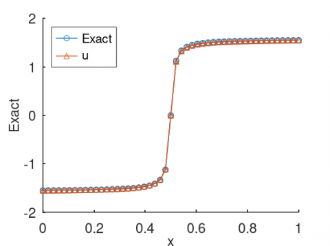
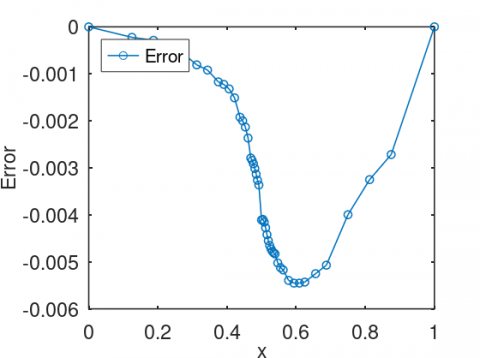
Table 1 shows the result of the analysis. From this table, it takes forty-eight elements for traditional FEM to arrive at an error value of 0.042372 while it takes h-adaptive FEM, forty-eight elements with four parental elements to arrive at an error value of 0.007007. It clearly shows that h-adaptive FEM is better compared to traditional FEM. Figures 3 and 4 shows the error graph of adaptive FEM and traditional linear FEM respectively. Figure 5 and Figure 6 shows the comparison of the exact solution and the numerical solution for the adaptive FEM and traditional FEM respectively.
Table 1. Comparison of the error of the two methods
|
Methods |
Error |
|
h-adaptive FEM with 48-elements |
0.007007 |
|
FEM with 48-elements |
0.042372 |
Figure 3. h-adaptive FEM error
Figure 4. Linear FEM error
Figure 5. h-adaptive FEM solution
Figure 6. Linear FEM solution
Example 2.
Given the following exact solution (refer to Eq. (1)),
$T=(1-x)\left(\tan ^{-1}\left(k\left(x-x_{0}\right)\right)+\tan ^{-1}\left(k x_{0}\right)\right)$,
$T(0)=0, T(1)=1, v=0, c=0, D=\frac{1}{a}+a\left(x-x_{0}\right)$
$f=2\left\{1+k\left(x-x_{0}\right)\left[\tan ^{-1}\left(x-x_{0}\right)+\tan ^{-1}\left(k x_{0}\right)\right]\right\}$,
Both the h-adaptive finite element method and the traditional finite method are also considered for this question to compare their error. Table 2 shows the result of the analysis, taking k=50 and x0=0.5.
Table 2. Comparison of the error of the two methods
|
Methods |
Error |
|
h-adaptive FEM with 44-elements |
0.001740 |
|
FEM with 44-elements |
0.017763 |
Figure 7. h-adaptive FEM error
Figure 8. Linear FEM error
Figure 9. h-adaptive FEM solution
Figure 10. Linear FEM solution (h=1/20)
Table 2 above shows that it takes forty-four elements for traditional FEM to arrive at an error value of 0.017763 while it takes h-adaptive FEM, forty-eight elements with four parental elements to arrive at an error value of 0.001740. It clearly shows that h-adaptive FEM is better compared to traditional FEM. Figures 7 and 8 above shows the error graph of adaptive FEM and traditional linear FEM respectively. Figure 9 and Figure 10 above shows the comparison of the exact solution and the numerical solution for the adaptive FEM and traditional FEM respectively.
3.1 Error analysis
This section focuses on the truncation error of the displacement. The error of the finite element method with constant mesh is considered. Truncation error through Taylor series expansion is expressed as shown below.
From Eq. (3) above, we have,
$\left.w \cdot D \frac{\partial u}{\partial x}\right|_{0} ^{L}-\int_{0}^{L} D \frac{\partial w}{\partial x} \frac{\partial u}{\partial x} d x-\int_{0}^{L} w \cdot v \frac{\partial u}{\partial x} d x$
$+\int_{0}^{L} w \cdot c(x) u(x) d x=\int_{0}^{L}(w \cdot f) d x$ (14)
substitute for:
$u=u_{h}+\frac{h^{2}}{2 !} u^{\prime \prime}\left(x^{*}\right), u^{\prime}=u_{h}^{\prime}+\frac{h^{2}}{2 !} u^{\prime \prime \prime}\left(x^{*}\right), \quad x^{*} \in(0, L)$
in Eq. (14) above gives,
$\left.w \cdot D\left(\frac{\partial}{\partial x} u_{h}+\frac{h^{2}}{2} u^{\prime \prime \prime}\left(x^{*}\right)\right)\right|_{0} ^{L}-\int_{0}^{L} D \cdot \frac{\partial w}{\partial x}$$\cdot\left(\frac{\partial}{\partial x} u_{h}+\frac{h^{2}}{2} u^{\prime \prime \prime}\left(x^{*}\right)\right) d x$$-\int_{0}^{L} w \cdot v \cdot\left(\frac{\partial}{\partial x} u_{h}+\frac{h^{2}}{2} u^{\prime \prime \prime}\left(x^{*}\right)\right) d x$$+\int_{0}^{L} w \cdot c(x) \cdot\left(u_{h}+\frac{h^{2}}{2} u^{\prime \prime}\left(x^{*}\right)\right) d x$ $=\int_{0}^{L}(w \cdot f) d x$ (15)
$w=N \phi \equiv N_{i}, \quad i \in I N, \quad w(0)=0$
where, IN represents internal and Neuman boundary nodes.
$\left.w(L) \cdot D \cdot \frac{\partial u_{h}}{\partial x}\right|_{0} ^{L}+w(L) \cdot D \cdot \frac{h^{2}}{2} u^{\prime \prime \prime}\left(x^{*}\right)$
$-\int_{0}^{L} D \cdot \frac{\partial w}{\partial x} \frac{\partial u_{h}}{\partial x} d x-\int_{0}^{L} D \cdot \frac{\partial w}{\partial x} \cdot \frac{h^{2}}{2} u^{\prime \prime \prime}\left(x^{*}\right) d x$
$-\int_{0}^{L} w \cdot v \frac{\partial u_{h}}{\partial x} d x-\int_{0}^{L} w \cdot v \cdot \frac{h^{2}}{2} u^{\prime \prime \prime}\left(x^{*}\right) d x$
$+\int_{0}^{L} w \cdot c(x) \cdot u_{h} d x+\int_{0}^{L} w \cdot c(x) \cdot \frac{h^{2}}{2} u^{\prime \prime}\left(x^{*}\right) d x=\int_{0}^{L}(w \cdot f) d x$
Re-arrange, we have,
$-\int_{0}^{L} D \cdot \frac{\partial N_{i}}{\partial x} \cdot \frac{\partial u_{h}}{\partial x} d x-\int_{0}^{L} N_{i} \cdot v \frac{\partial u_{h}}{\partial x} d x+\int_{0}^{L} N_{i} \cdot c(x) u_{h} d x$
$=\int_{0}^{L} N_{i} \cdot f d x+\int_{0}^{L} D \cdot \frac{\partial N_{i}}{\partial x} \cdot \frac{h^{2}}{2} u^{\prime \prime \prime}\left(x^{*}\right) d x$
$+\int_{0}^{L} N_{i} \cdot v \cdot \frac{h^{2}}{2} u^{\prime \prime \prime}\left(x^{*}\right) d x-\int_{0}^{L} N_{i} \cdot c(x) \cdot \frac{h^{2}}{2} u^{\prime \prime}\left(x^{*}\right) d x$
$-\left.N_{i}(L) \cdot D \cdot \frac{\partial u_{h}}{\partial x}\right|_{L}-N_{i}(L) \cdot D \cdot \frac{h^{2}}{2} u^{\prime \prime \prime}\left(x^{*}\right)$
$-\sum_{j}^{n}\left(\int_{0}^{L} D \cdot \frac{\partial N_{i}}{\partial x} \cdot \frac{\partial N_{j}}{\partial x} d x\right) u_{j}-\sum_{j}^{n}\left(\int_{0}^{L} N_{i} \cdot v \cdot \frac{\partial N_{j}}{\partial x} d x\right) u_{j}$
$+\sum_{j}^{n}\left(\int_{0}^{L} N_{i} \cdot c(x) \cdot N_{j} d x\right) u_{j}$
$=\int_{0}^{L} N_{i} \cdot f d x+\int_{0}^{L} D \cdot \frac{\partial N_{i}}{\partial x} \cdot \frac{h^{2}}{2} u^{\prime \prime \prime}\left(x^{*}\right) d x$
$+\int_{0}^{L} N_{i} \cdot v \cdot \frac{h^{2}}{2} u^{\prime \prime \prime}\left(x^{*}\right) d x-\int_{0}^{L} N_{i} \cdot c(x) \cdot \frac{h^{2}}{2} u^{\prime \prime}\left(x^{*}\right) d x-\left.N_{i}(L) \cdot D \cdot \frac{\partial u_{h}}{\partial x}\right|_{L}-N_{i}(L) \cdot D \cdot \frac{h^{2}}{2} u^{\prime \prime \prime}\left(x^{*}\right)$
Let
$D_{i j}=\int_{0}^{L} D \cdot \frac{\partial N_{i}}{\partial x} \cdot \frac{\partial N_{i}}{\partial x} d x, \quad v_{i j}=\int_{0}^{L} N_{i} \cdot v \cdot \frac{\partial N_{j}}{\partial x} d x$,
$c_{i j}=\int_{0}^{L} N_{i} \cdot c(x) N_{j} d x, \quad k_{i j}=-D_{i j}-v_{i j}+c_{i j}$,
We have,
$\sum_{i=1}^{n} k_{i j} u_{j}=\int_{0}^{L} N_{i} \cdot f d x+\frac{D h^{2}}{2} u^{\prime \prime \prime}\left(x^{*}\right)\left(N_{i}(L)\right)+v$
$\cdot \frac{h^{2}}{2} \int_{0}^{L} u^{\prime \prime \prime}\left(x^{*}\right) N_{i} d x$
$-\frac{h^{2}}{2} \int_{0}^{L} u^{\prime \prime}\left(x^{*}\right) N_{i} \cdot c(x) d x$
$-\left.N_{i}(L) \cdot D \cdot \frac{\partial u_{h}}{\partial x}\right|_{L}$
$-N_{i}(L) \cdot D \cdot \frac{h^{2}}{2} u^{\prime \prime \prime}\left(x^{*}\right)$ (16)
$N_{a}=\left[\left.N_{i}\right|_{0} ^{L}\right]=N_{i}(L), \quad N_{b}=\left[\int_{0}^{L} N_{i} \cdot f d x\right]$,
$N_{c}=\left[\int_{o}^{L} u^{\prime \prime}\left(x^{*}\right) N_{i} \cdot c(x) d x\right], \quad i \in I N(i \neq 0)$
Therefore,
$N_{a}=\left[\begin{array}{c}0 \\ \vdots \\ 1\end{array}\right]$
$K u=f+\frac{D h^{2}}{2} u^{\prime \prime \prime}\left(x^{*}\right)\left[\begin{array}{c}0 \\ \vdots \\ 1\end{array}\right]+v \frac{h^{2}}{2} u^{\prime \prime \prime}\left(x^{*}\right) N_{b}-\frac{h^{2}}{2} N_{c}$
$-\frac{D h^{2}}{2}\left[\begin{array}{c}0 \\ \vdots \\ u^{\prime \prime \prime}\left(x^{*}\right)\end{array}\right]$ (17)
$K u=f+\Delta f$
where,
$\Delta f=\frac{D h^{2}}{2} u^{\prime \prime \prime}\left(x^{*}\right)\left[\begin{array}{c}0 \\ \vdots \\ 1\end{array}\right]+v \frac{h^{2}}{2} u^{\prime \prime \prime}\left(x^{*}\right) N_{b}-\frac{h^{2}}{2} N_{c}$
$-D \frac{h^{2}}{2}\left[\begin{array}{c}0 \\ \vdots \\ u^{\prime \prime \prime}\left(x^{*}\right)\end{array}\right]$ (18)
||$\Delta f|| \leq h^{2}\left|u^{\prime \prime \prime}\left(x^{*}\right)\right|\left(D+\frac{v}{2}|| N_{b}||\right)+\frac{h^{2}}{2}\left|u^{\prime \prime}\left(x^{*}\right)\right||| N_{c}||$ (19)
Theorem 1:
Given a linear system $A x=$ b where $A \in R^{n \times n}, b \in R^{n}$ and $x \in R^{n}$ With condition number given as $k(A)$. Let $\delta b \in R^{n}$ be a small perturbation of $b$ and define $x+\delta x \in R^{n}$ as the solution of the system:
$A(x+\delta x)=(b+\delta b)$,
Then,
$\frac{|| \delta x||}{|| x||} \leq k(A) \leq \frac{|| \delta b||}{|| b||}$
This can be written as,
$\frac{|| \delta b||}{k(A)|| b||} \leq \frac{|| \delta x||}{|| x||} \leq \frac{k(A)|| \delta b||}{|| b||}$
Apply the theorem above to Equation (19), we have,
$\frac{|| \delta f||}{k(A)|| f||} \leq \frac{|| \delta u||}{|| u||} \leq \frac{k(A)|| \delta f||}{|| f||}$
where, $k(A)$ is the condition number.
The error analysis is performed in the post-processing stage. For the simplicity of the calculation, it is assumed that:
$\left|u^{\prime \prime \prime}\left(x^{*}\right)\right| \overrightarrow{\max }\left|u^{\prime \prime \prime}(x)\right|$
Table 3. Error analysis for linear elements
|
|
$\frac{|| \delta f||}{k(A)|| f \|}$ |
$\frac{|| \delta x||}{|| x||}$ |
$\frac{k(A)\|\delta f\|}{\|f\|}$ |
$k(A)$ |
|
Ex 1. |
6.8341e-08 |
3.0954e-04 |
0.23353 |
584.56 |
|
Ex 2. |
7.1111e-07 |
0.030277 |
0.1481 |
456.35 |
From Table 3 above, it is evident that when the condition number of matrix $K$ is increased, then the relative error increases. In conclusion, two factors affect the error accuracy, which is $\Delta x$ and condition number of matrix $K$.
In this study, h-adaptive and traditional finite element method that enables high accurate approximations of high gradient advection-dominated problems have been proposed. The h-adaptive quickly identifies the fine region and concentrates in that region by further subdivide the area without further increase the elements to get better accuracy. This has also saved time and computational stress and minimizes error compared to the traditional finite element method, which requires more time and computational stress to deal with the generated algebraic equation due to the many elements involved. This approach is recommended for general differential equations with high gradients.
|
k |
condition number |
|
f |
load vector |
|
K |
stiffness matrix |
|
h |
mesh |
|
D |
conductivity |
|
w |
weight function |
|
N |
shape function |
|
Greek symbols |
|
|
$\alpha$ |
high-gradient value |
|
$\delta$ |
change |
[1] Lin, J., Xu, Y., Zhang, Y. (2020). Simulation of linear and nonlinear advection–diffusion–reaction problems by a novel localized scheme. Applied Mathematics Letters, 99: 106005. https://doi.org/10.1016/j.aml.2019.106005
[2] Bachini, E., Farthing, M.W., Putti, M. (2021). Intrinsic finite element method for advection-diffusion-reaction equations on surfaces. Journal of Computational Physics, 424: 109827. https://doi.org/10.1016/j.jcp.2020.109827
[3] Arqub, O.A. (2018). Numerical solutions for the Robin time-fractional partial differential equations of heat and fluid flows based on the reproducing kernel algorithm. International Journal of Numerical Methods for Heat & Fluid Flow, 28(4). https://doi.org/10.1108/HFF-07-2016-0278
[4] Li, C., Chen, A. (2018). Numerical methods for fractional partial differential equations. International Journal of Computer Mathematics, 95(6-7): 1048-1099. https://doi.org/10.1080/00207160.2017.1343941
[5] Li, J., Chen, Y.T. (2019). Computational Partial Differential Equations Using MATLAB®. CRC Press.
[6] Jeong, S., Kim, M.Y. (2021). Computational aspects of the multiscale discontinuous Galerkin method for convection-diffusion-reaction problems. Electronic Research Archive, 29(2): 1991-2006. http://dx.doi.org/10.3934/era.2020101
[7] Bischoff, M., Bletzinger, K.U., Wall, W.A., Ramm, E. (2004). Models and finite elements for thin-walled structures. Encyclopedia of Computational Mechanics, 1-86. https://doi.org/10.1002/0470091355.ecm026
[8] Abbas, S., Alizada, A., Fries, T.P. (2010). The XFEM for high-gradient solutions in convection-dominated problems. International Journal for Numerical Methods in Engineering, 82(8): 1044-1072. https://doi.org/10.1002/nme.2815
[9] Zhao, X., Hu, X., Cai, W., Karniadakis, G.E. (2017). Adaptive finite element method for fractional differential equations using hierarchical matrices. Computer Methods in Applied Mechanics and Engineering, 325: 56-76. https://doi.org/10.1016/j.cma.2017.06.017
[10] Giere, S., Iliescu, T., John, V., Wells, D. (2015). SUPG reduced order models for convection-dominated convection–diffusion–reaction equations. Computer Methods in Applied Mechanics and Engineering, 289: 454-474. https://doi.org/10.1016/j.cma.2015.01.020
[11] Antonietti, P.F., Cangiani, A., Collis, J., Dong, Z., Georgoulis, E.H., Giani, S., Houston, P. (2016). Review of discontinuous Galerkin finite element methods for partial differential equations on complicated domains. In Building Bridges: Connections and Challenges in Modern Approaches to Numerical Partial Differential Equations, pp. 281-310. https://doi.org/10.1007/978-3-319-41640-3_9
[12] Burman, E., Hansbo, P., Larson, M.G., Massing, A. (2018). Cut finite element methods for partial differential equations on embedded manifolds of arbitrary codimensions. ESAIM: Mathematical Modelling and Numerical Analysis, 52(6): 2247-2282. https://doi.org/10.1051/m2an/2018038
[13] Ooi, E.T., Man, H., Natarajan, S., Song, C. (2015). Adaptation of quadtree meshes in the scaled boundary finite element method for crack propagation modelling. Engineering Fracture Mechanics, 144: 101-117. https://doi.org/10.1016/j.engfracmech.2015.06.083
[14] Nguyen-Xuan, H., Nguyen-Hoang, S., Rabczuk, T., Hackl, K. (2017). A polytree-based adaptive approach to limit analysis of cracked structures. Computer Methods in Applied Mechanics and Engineering, 313: 1006-1039. https://doi.org/10.1016/j.cma.2016.09.016
[15] O’Hara, P., Hollkamp, J., Duarte, C.A., Eason, T. (2016). A two-scale generalized finite element method for fatigue crack propagation simulations utilizing a fixed, coarse hexahedral mesh. Computational Mechanics, 57(1): 55-74. https://doi.org/10.1007/s00466-015-1221-7
[16] Mitchell, W.F., McClain, M.A. (2011). A survey of hp-adaptive strategies for elliptic partial differential equations. In Recent Advances in Computational and Applied Mathematics, pp. 227-258. https://doi.org/10.1007/978-90-481-9981-5_10
[17] Morin, P., Nochetto, R.H., Pauletti, M.S., Verani, M. (2012). Adaptive finite element method for shape optimization*. ESAIM: Control, Optimisation and Calculus of Variations, 18(4): 1122-1149. https://doi.org/10.1051/cocv/2011192
[18] Witkowski, T., Ling, S., Praetorius, S., Voigt, A. (2015). Software concepts and numerical algorithms for a scalable adaptive parallel finite element method. Advances in Computational Mathematics, 41(6): 1145-1177. https://doi.org/10.1007/s10444-015-9405-4
[19] Yu, T., Bui, T.Q. (2018). Numerical simulation of 2-D weak and strong discontinuities by a novel approach based on XFEM with local mesh refinement. Computers & Structures, 196: 112-133. https://doi.org/10.1016/j.compstruc.2017.11.007
[20] Saloustros, S., Cervera, M., Pelà, L. (2019). Challenges, tools and applications of tracking algorithms in the numerical modelling of cracks in concrete and masonry structures. Archives of Computational Methods in Engineering, 26(4): 961-1005. https://doi.org/10.1007/s11831-018-9274-3