Khalideh Al Bkoor Alrawashdeh* | Kamel K. Al-Zboon | Zakaria Al Qodah
© 2021 IIETA. This article is published by IIETA and is licensed under the CC BY 4.0 license (http://creativecommons.org/licenses/by/4.0/).
OPEN ACCESS
Desalination processes are considered an essential solution to meet the water scarcity in Jordan. Among the desalination techniques, the multistage flash (MSF) desalination technique has a significant contribution to water budget in many regions around the world. In this paper, MSF with a mixing brine desalination plant was proposed in Aqaba city of Jordan. The plant will consume 5 MW power to produce about 74 Kg/s of freshwater. Different designs are studied to determine the most appropriate design. Also, the effect of feed sea water flow rate, heating steam flow rate and number of stages on the plant performance were evaluated. The optimum layout consists of 24 stages with 3.6 m width, 2.6 m length, and with a recycled brine flow rate of about 651 Kg/s. The expected plant performance is 9.6.
desalination, MSF desalination, mixing brine, desalination plant design, dimension
Jordan is almost an arid country with 89342 km² land area and a population of 10.2 million, which is expected to almost double by 2050 with a recent average growth rate of about 2.08% [1]. Water resources in Jordan are characterized by variability, scarcity, and uncertainty because they depend on rainfall. The per capita share of renewable water resources is 100 m³/capita/year. Therefore, Jordan is listed as the fourth poorest country regarding water resources worldwide [2-4].
The existing water deficit and the scarcity of freshwater resources in Jordan are increasing: as a result of: the fast rate of population increase, the expansion of both the industrial and agricultural sectors, and refugees’ influxes of Palestinians, Iraqis and Syrian’s refugees. This adversely affected Jordan's economy, agricultural activities, agricultural activities and social life. Accordingly, seawater desalination provides a practical solution to water scarcity and may form a very important component of Jordan’s water budget [2].
Seawater desalination has been defined as the removal of dissolved salts from a virtually limitless supply of seawater in order to make it suitable for human consumption as well as industrial and agricultural uses [3-5]. In the desalination process, the saline water is separated into two streams; one that has low salt concentrations (freshwater) and the other with high salt concentrations (brine) [5-7]. Several desalination technologies were used around the world; thermal distillation and membrane separation are the two major types of these technologies [3, 5, 7]. Thermal technology was classified broadly into two subcategories: multistage flash (MSF) and multiple effect distillation (MED) processes [8-12]. Most literature characterized the MSF as high energy consumption technology, in the range of 1.5 – 2 kg/s [ 2, 9-11]. Khoshgoftar Manesh et al. [9] reported that the generated power using MSF plant is lower than MED plant (1.5 kg/s versus 1kg/s).
In MSF distillation plants the distillation process is achieved by using several successive chambers (15- 25 stages) [13]. Through the operation of each successive stage of the plant, the pressure is gradually reduced; hence the temperature is increased. Firstly, the feed water is heated under high pressure and is driven to the first flash chamber at a lower pressure [8-11]. Due to the pressure dropping, the water rapidly boils resulting in sudden evaporation or flashing, each stage pressure is lower than the previous stage, resulting in the continuous flashing process through the stages [14, 15].
The generated vapor is condensed on heat exchanger tubing to convert it into freshwater [5, 8, 16]. The flashing flow system in the MSF process can be either a once-through or with a brine recirculation [12, 14, 15]. The recycled brine MSF system contains three sections: brine heater, heat recovery section, and the brine mixing tank. The recycled brine stream flows in the opposite direction of the distillate product in the flashing stages [17]. The temperature of recycled brine increased in the brine heater by saturated steam to the top brine temperature [17, 18]. The heated brine then passes from the first to the subsequent stages, creating a small amount of freshwater at each stage [16-19]. The flashing process converts the extra sensible heat of the regenerated brine into latent heat for vapor production [19, 20]. The brine salinity rises as the water evaporates, but it is limited to 70,000 ppm to avoid scaling. As the concentrated brine leaves the final stage, part of it is recycled to the sea to control the salinity system, while the rest is recycled for heat recovery, thermal efficiency improvement, and to reduce the feed water flow rate [12-17].
In the literature, many researchers investigate the MSF processes [21, 22]. Said [16] developed a steady-state mathematical model of an MSF desalination plant using gPROMS software to investigate the operation parameters (flow rate of below down brine and brine recycle and steam temperature). He reported that the steam temperature had a great effect on preserving the production rate of freshwater at different seasons. Hanshik et al. [23] evaluated the design fundamentals and performance (Pr) of the MSF distillation plant by varying the operational conditions. The results showed that the Pr increased as the top brine temperature (TBT) increased, and that the energy consumption may be regulated by modifying the operating conditions. Alrawashde et al. [24] also investigated technical and economic issues of a small-scale plant of MSF - Recycle Brine, plant has 24 stages and produces 383 m3/day of distillate water. They stated that as the stage number increases, so would the capital cost and Pr. Hassanean et al. [25] presented a mathematical model and MATLAB code to analyze Pr of MSF system with supporting correlations - physical factors. The software was used to predicate and trace the plant efficiency. Gao et al. [26] presented a simulation study to identify the seawater temperature sensitivity and its effect on the system gain. They concluded that the optimal operation of MSF was studied with two different objective functions. The maximum GOR (Pr) in conjunction with the steam temperature of 97 ℃, and the steam flow rate and temperature increase as the demand for fresh water increases.
Moreover, several researchers discussed a new approach of MSF plant with several power sources [17, 24]. MSF plant powered by solar system were studied [27, 28], Al-Othman et al. [28] established a simulation study for a novel solar-driven MSF desalination plant in UAE. The study aimed to examine the use of parabolic trough collectors (PTC) and a solar pond to fully satisfy the energy requirements for MSF desalination. It was found that the use of two PTCs of a total aperture area of 3160 m2 could provide about 76% of the power requirements. The remaining 24% of these requirements can be obtained by a solar pond of a surface area of 0.53 km2. Furthermore, MSF desalination plant is powered by a biomass plant, where the brine heater is driven by biogas as the main fuel [24]. Also, A MATLAB code was created by Al Ghamdi and Mustafa [29] to analyze exergy destruction in an MSF desalination plant in Saudi Arabia. The major exergy destruction was determined at the heat Recovery Section with very low efficiency. MSF units are generally made up of many flash stages to improve the system's energy efficiency [24, 28-33], with the total number of stages ranging from 15 to 25 [16, 24-29]. This technique can meet a freshwater demand of 4000 to 57,000 m3/day, with heating temperatures ranging from 90 to 110℃ [30]. A few modifications have been made in more recent plants. In instead of the heat rejection section and condenser with 2 to 3 flash stages is added. [15, 22-25]. In some studies, saltwater is utilized as a cooling fluid. After this phase, a portion of the saltwater is discarded, while the remainder is combined with brine recovered during the final flash stage [18, 22, 27]. The salt solution is utilized in the desalination unit's main section. This approach is used to improve the energy efficiency of large desalination scale [31, 32], which are made up of 19–40 stages of heat recovery section and 2–3 stages of heat rejection section [24, 28]. Scaling control (adding chemicals) [11], the development of automation [17, 24] and control systems [22-27], and the use of better materials for the construction of desalination units have all enhanced the system's dependability during the previous two decades [30]. Exergy analysis has recently been presented in a number of studies [33-37] to enhance the energy efficiency of desalination systems. In this light, an effective method for recommending ideas to enhance the energy efficiency of existing desalination devices is an efficiency study done in accordance with the Second Thermodynamic Law [33, 36, 37].
Other researchers focused on MSF with brine mixing system (MSF-M), El-Dessouky et al. [38] proposed this system to reduce the energy losses. The Pr was analyzed as a function of the TBT, the temperature of the unevaporated brine recycle, and the number of stages. Then El-Dessouky et al. [39] provided an overview of the MSF process that aimed to reduce the production cost. Also, a summary of the novel MSF-M system was presented. An analysis of the interactions and functions of various MSF systems was performed. They reported that the MSF-M system showed higher thermal performance ratios compared with conventional MSF. Mussati et al. [40] investigated a design optimization model to improve the structure of an MSF system, and the problem was solved using the GAMS platform's extended gradient method. Lappalainen et al. [41] introduced a new one-dimensional modeling and dynamic simulation approach for MSF-B. The method combines simultaneous mass, momentum, and energy solutions, Rachford-Rice equation local phase equilibrium, and rigorous calculations of seawater characteristics as a function of salinity, pressure, and temperature.
Also, Alhazmy [42] presented a modified MSF- M plant. Part of the leaving brine was mixed with fresh seawater feed and before entering the bottom stage feed heater; it was cooled to low temperature. The results show that distillate yield was improved by 1.18%-1.4% for every 1℃ reduction in the temperature of the plant bottom and the modified MSF-MC demonstrated an expanded evaporation range and preserved the basic advantages of low chemical treatment and feed pumping compared to the conventional MSF plant. In subsequent research, Alhazmy [43] presented a thermal and economic analysis for the modified MSF-MC. The results proved that attaching a cooling unit to the MSF plant is a promising and cost-effective technique.
The installation of a thermal desalination plant is planned to be in Aqaba in Jordan which is the only coastal city. The city has one of the highest population growth rates in Jordan, which is estimated to be 148,398 [44]. Aqaba has a desert climate with a warm winter and a hot dry summer. Moreover, it is the most appropriate city to construct the plant with availability of seawater and less energy consumption due to its location and climate.
This study presents a proposed medium scale MSF-M desalination plant to provide freshwater and serve the residents of Aqaba city. The plant design that is proposed comprises 24 stages (3.6 m of width and 2.6 of length for each stage), brine heater with a high heating steam flow rate and a mixing unit. The feed seawater will be pumped from the Red sea at a rate of 178 Kg/s and salinity concentration of 41,000 ppm. Mathematical model was applied to evaluate the technical characteristics of the plant. Firstly, the modeled desalination plant was divided into module of brine heater, modules of flash stage modules, and module of mixer, and split modules, with equations created and put together to represent the entire process model based on energy and mass conservation principles. Then, it is based on the fundamental rules of mass balance, energy balance, and heat transfer equations, as well as physical property correlations. The performance ratio, heating load, temperature profile, streams flow rate, stage dimensions and distillated capacity were evaluated and obtained. The MSF-M plant is analyzed as a function of number of flashing stages, feed seawater flowrate and heating steam flowrate. Analyses are performed over stages with a temperature range of 34 -110℃. The operation factors were chosen to improve the below down - brine salinity limited to less than 70,000 ppm. The temperature range and energy consumption were executed with different operation factors to optimize the Pr and improve freshwater production up to 70 kg/s.
2.1 Variables and assumptions
Multistage flash with mixing brine (MSF-M) distillation plant is designed to cover the freshwater demand in Aqaba. The proposed MSF-M plant consists of 24 flashing stages and a brine heater. The flashing stages are considered as the heat recovery section while the brine heater is the heat rejection section. The stages shape is selected to be rectangular while the brine heater is shell and tube, heat exchanger. Several constants and assumptions are considered in the design of the MSF-M plant. The plant is designed to be supplied by 5 MW power. The salinity of the feed seawater (Xf) is considered 41,000 ppm salt concentration [44] while the rejected brine salinity (Xb) is 70,000 ppm [44]. The produced distillate flowrate (Md) is assumed to be delivered to the consumers for drinking and industrial purposes. Various temperature values are considered such as top brine temperature (To), temperature of heating stream (Ts), seawater feed temperature (Tf) and the blowdown temperature (Tn), as shown in Table 1 [40].
Table 1. Assumed parameters to evaluate multistage mixing brine plant
|
Parameter |
Value |
Ref |
Parameter |
Value |
Ref |
|
Xf, ppm |
41,000 |
[33] |
Tf, ℃ |
18 |
[33, 34] |
|
Xb, ppm |
70,000 |
[33] |
Tn, ℃ |
40 |
[34] |
|
T0, ℃ |
110 |
[12, 17, 33] |
Vb,kg/m.s |
180 |
[35] |
|
Ts, ℃ |
160 |
[12] |
Cd |
0.2 |
[35] |
|
CP, Kj/kg.K |
4.18 |
[12, 17, 33, 34] |
Vn, m/s |
6 |
[17] |
Also, the brine mass flow rate per stage width (Vb), heat capacity of liquid steam (Cp), the friction coefficient (Cd) and the vapor velocity in the last stage (Vn) are assumed as presented in Table 1 according to the literature. The latent heat of steam (ʎs) and condensing vapor (ʎv) are obtained from steam tables according to the assumed temperature, as mentioned before, which are 2081.86 kJ/kg and 2320.63 kJ/kg, respectively [17].
2.2 Temperature profile of each stage
The average temperature (Tav) and the value of the temperature drop per each stage (∆Ts) are calculated by the following equation [45]:
$T_{A V}=\frac{T_{0}-T_{n}}{2}$ (1)
$\Delta T_{S}=\frac{T_{0}-T_{n}}{n}$ (2)
where, Tn (℃) is brine temperature at last stage, T0 (℃) is the top brine temperature, and n is the stage number.
The specific ratio of sensible heat and latent heat (Y) can be obtained using Eq. (3).
$Y=\frac{C_{P} \cdot \Delta T_{S}}{ʎ_{v}}$ (3)
where, the Cp (Kj/kg.k). is the specific heat value at constant pressure, and ʎv(Kj/kg) is the average latent heat cross the stages.
The seawater temperature which leaves the condenser of the first stage (t1) and the second stage (t2) is determined as the following [44-48]:
$t_{1}=T_{r}+n \cdot \Delta T_{S}$ (4)
$t_{i}=t_{i-1}-\Delta T_{S}$ (5)
This relation shows that the drop in the total temperature of the flashing brine is equivalent to the total temperature gain of the brine recycle flowing inside the tube of the preheater/condenser.
The brine temperature that leaves the stage (brine pool within the stage) can be calculated using Eqns. (6) and (7).
$T_{i}=T_{i-1}-i \cdot \Delta T_{S}$ (6)
$T_{2}=T_{1}+n \cdot \Delta T_{S}$ (7)
$T_{0}-T_{1}=\Delta T_{S}+\Delta T_{\text {loss }}$ (8)
where, i is the stage number, n is the number of the stages and ∆Tloss is the thermodynamic losses, which are the temperature difference between the temperature of the brine leaving the stage, and the temperature of the condensation vapor temperature, which is caused by pressure drop, non-equilibrium allowance and the boiling point elevation.
2.3 Flow rate of streams and the main parameters
The specific steam mass flow rate (Ms) is used to increase the recycle brine which leaves the first condenser at the top brine temperature To, which is required to drive the flashing process across the stages. MS is computed using Eq. (9).
$M_{S}=\frac{Q \cdot \rho}{C_{P} \cdot \Delta T}$ (9)
where, Q is the heat energy supplied to the system by brine heater, KJ, ʎs is the latent heat of the steam which drive MSF-M process and λav is the average latent heat at the average temperature [45].
The value of the recycle brine mass flow (Mr) is determined by the amount of heat added in the brine heater section and the temperature difference between the top brine temperature and the brine temperature that exits the first condenser. The specific flow rate of recycle brine stream can be calculated as Eq. (10) [49].
$M_{r}=\frac{m_{s} \cdot ʎ_{S}}{C_{P} \cdot\left(T_{0}-t_{1}\right)}$ (10)
The flow rate of accumulation distillated Md is based on the flow rate of feed water and recycle brine, this can be calculated by the following equation.
$M_{d i}=M_{r}\left(1-(1-Y)^{i-1}\right)$ (11)
The specific flow rate of the feed water (Mf) and brine flow are determined by Eqns. (12) and (13), respectively.
$M_{f}=\frac{X_{b} \cdot M_{d}}{\left(X_{b}-X_{f}\right)}$ (12)
$M_{b}=M_{r}-\sum M_{d i}$ (13)
where, Xb and Xf are the salt concentration (ppm) of the brine and feed water, respectively.
The performance ratio (Pr) is calculated as the ratio of distillated product to the seam flow rate across the brine heater, the Pr can be calculated by Eq. (14).
$P_{r}=\frac{M_{d}}{M_{S}}$ (14)
The salinity of feed seawater and the salinity of the brine at each stage can be obtained by Eqns. (15) and (16):
$X_{f}=\frac{M_{r} X_{r}-\left(M_{r}-M_{f}\right) X_{n}}{M_{f}}$ (15)
$X_{i}=\frac{M_{r} X_{r}}{M_{b}}$ (16)
where the Xn below down salinity.
2.4 Stage dimensions
The stages width (w) and the stage length (L) are determined by Eqns. (17) and (18), respectively [49].
$\mathrm{W}=\frac{\mathrm{M}_{\mathrm{r}}}{\mathrm{V}_{\mathrm{b}}}$ (17)
$L=\frac{M_{d}}{\rho_{v n} \cdot V_{n} \cdot w}$ (18)
where, w is the stage length (m), the L is the stage length (m), Vb is the brine flow mass per stage width (kg/m.s), Vn is the velocity of the steam produced at the last stage (m.s), and ρvn is the density of the steam in the last stage (kg/m3).
The cross-sectional area (As) for each stage of the plant is calculated using Eq. (19) [10].
$A_{S}=w . L$ (19)
Whereas the cross-sectional area (m2).
Also, the stage dimensions consist of gate height (GH), the height of the brine pool (H), both can be calculated by Eqns. (20) and (21).
$G H_{i}=M_{r}\left(2 \rho_{b i} \cdot \Delta P_{i}\right)^{\frac{-0.5}{w . C_{d}}}$ (20)
$H_{i}=0.2+G H_{i}$ (21)
where, ρbi is the density of brine (kg/m3), Cd is the discharge coefficient of the weir and ∆P is the drop pressure (bar).
The temperature of the vapor produced in each stage can be calculated by the following equation [8, 10].
$T_{V i}=T_{i}-B P E_{i}-N E A_{i}-\Delta T_{d i}$ (22)
where, the ΔTdi is the temperature drop in the demister, which is assumed to be negligible in comparison with the values of NEAi and BPEi.
The non-equilibrium allowance (NEA) and the boiling point elevation (BPE) are necessary to obtain the temperature of the steam condensation for each stage. NEA (℃) and BPE (℃) are calculated using Eqns. (22)-(26) [8, 10, 37, 42].
$N E A_{i}=(0.9784)^{T_{0}}(15.7378)^{H_{i}}(1.3777)^{10^{-6} . v_{b}}$ (23)
$B=\left(6.71+6.34 \times 10^{-2} \times T_{i}+9.74 \times 10^{-5} \times T_{i}^{2}\right) \times 10^{-3}$ (24)
$C=\left(22.238+9.59 \times 10^{-3} \times T_{i}+9.42 \times 10^{-5} \times T_{i}^{2}\right) \times 10^{-3}$ (25)
$B P E_{n}=X_{n}\left(B+X_{n} C\right) \times 10^{-3}$ (26)
where, B and C are constants.
The brine heater (Ab):
$A_{b}=\frac{M_{S} ʎ_{S}}{U_{b} L M T D_{b}}$ (27)
where, Ub is the overall brine heater heat transfer coefficient, this can be calculated using the following equation.
$U_{b}=1.7+3 \times 10^{-3} \times T_{S}-1.99 \times 10^{-7} T^{3}$ (28)
And LMTDb is the log mean temperature difference which can be calculated by Eq. (29).
$L M T D_{b}=\frac{\left(T_{S}-T_{o}\right)-\left(T_{S}-t_{1}\right)}{\ln \left(\frac{T_{S}-T_{0}}{T_{S}-t_{1}}\right)}$ (29)
The condenser heat transfer area (Ac) is obtained using the following equation:
$A_{C}=\frac{M_{r} C_{p}\left(t_{1}-t_{2}\right)}{U_{C} L M T D_{C}}$ (30)
where, Uc is the overall condenser heat transfer coefficient, this can be determined using the following equation:
$U_{c}=1.719+3.2063 \times 10^{-3} \times T_{V}+1.5971 \times 10^{-5} \times T_{V}^{2}-1.9918 \times 10^{-7} \times T_{V}^{3}$ (31)
And the LMTDc is the log mean temperature difference which can be calculated by Eq. (32).
$L M T D_{C}=\frac{\left(T_{V 1}-t_{1}\right)-\left(t_{V}-t_{2}\right)}{\ln \left(\frac{T_{V}-t_{1}}{T_{v}-t_{2}}\right)}$ (32)
The specific heat transfer area and the total specific heat transfer area for the condenser and the brine heater are calculated using the following equations [45, 46].
$A_{c} / M_{d}=\frac{M_{r} C_{p} \Delta T_{s}}{U_{C} L M T D_{C}}$ (33)
$A_{b} / M_{d}=\frac{ʎ_{s}}{P_{r} U_{b} L M T D_{b}}$ (34)
The total specific heat transfer for both brine heater and flashing stages can be obtained as the following:
$S_{A}=A_{b}+n \cdot A_{C}$ (35)
3.1 Stage characteristics
The temperatureinthe1st chamber and the 2nd chamber are determined by using Eqns. (6) and (7) respectively (the temperature depends on the top brine temperature). The resultant temperatures for all stages are shown in Table 2. Table 2 shows the temperature profile of feed water which passes through the condensers, the temperature of brine and the vapor produced inside each stage.
Table 2. Temperature values for the stages and the condenser
|
#n |
T out (℃) |
T in (℃) |
t out (℃) |
t in (℃) |
Tav (℃) |
|
1 |
107.09 |
110 |
103.84 |
100.93 |
105.00 |
|
2 |
104.17 |
107.09 |
100.93 |
98.02 |
102.05 |
|
3 |
101.25 |
104.18 |
98.02 |
95.11 |
99.14 |
|
4 |
98.34 |
101.27 |
95.11 |
92.2 |
96.22 |
|
5 |
95.42 |
98.36 |
92.2 |
89.29 |
93.28 |
|
6 |
92.51 |
95.45 |
89.29 |
86.38 |
90.39 |
|
7 |
89.59 |
92.54 |
86.38 |
83.47 |
87.45 |
|
8 |
86.67 |
89.63 |
83.47 |
80.56 |
84.54 |
|
9 |
83.76 |
86.72 |
80.56 |
77.65 |
81.59 |
|
10 |
80.84 |
83.81 |
77.65 |
74.74 |
78.69 |
|
11 |
77.93 |
80.9 |
74.74 |
71.83 |
75.78 |
|
12 |
75.01 |
77.99 |
71.83 |
68.92 |
72.82 |
|
13 |
72.09 |
75.08 |
68.92 |
66.01 |
69.94 |
|
14 |
69.18 |
72.17 |
66.01 |
63.1 |
66.95 |
|
15 |
66.26 |
69.26 |
63.1 |
60.19 |
64.09 |
|
16 |
63.35 |
66.35 |
60.19 |
57.28 |
61.12 |
|
17 |
60.43 |
63.44 |
57.28 |
54.37 |
58.10 |
|
18 |
57.51 |
60.53 |
54.37 |
51.46 |
55.11 |
|
19 |
54.60 |
57.62 |
51.46 |
48.55 |
52.34 |
|
20 |
51.68 |
54.71 |
48.55 |
45.64 |
49.18 |
|
21 |
48.77 |
51.8 |
45.64 |
42.73 |
46.37 |
|
22 |
45.85 |
48.89 |
42.73 |
39.82 |
43.39 |
|
23 |
42.93 |
45.98 |
39.82 |
36.91 |
40.45 |
|
24 |
40 |
43.07 |
36.91 |
34 |
37.41 |
The temperature of the feed water flowing within the condenser rises from the last stage toward the first stage as the brine temperature declines from the first stage toward the last stage. That is because the latent heat rejected from the brine will be absorbed by the water flow within the condenser. Also, the temperature increment was accompanied by a decrease in pressure.
The results are shown in Table 2, which presents the stages temperature profile and the seawater temperature that leaves the condenser for all stages. The temperature dropped in each stage by 2.91℃. Through the stages, the temperature dropped from 110℃ for the first stage to 43℃ for the 24th stage. Also, the temperature of seawater leaving the condenser dropped from 101℃ for the first stage to 34℃ for the 24th stage.
Table 3 illustrates all the characteristics of each stage and the main parameters that effect on the temperature.
As shown in Table 3, the recycled brine hence to reduce the flow rate of the feed seawater which led to recovering a portion of the heat added to the brine heater of the system. It also improves the efficiency of the process. Across the stages the quantity of the distillated water decreased gradually, and the salinity increased up to 7000 ppm.
Table 3. Distillate flow rate, brine flow rate and salt concentration for all stages
|
#n |
Mdi (kg/s) |
ƩMdi |
Mb (kg/s) |
Xi (ppm) |
|
1 |
3.257 |
3.257 |
648.103 |
61756.25 |
|
2 |
3.241 |
6.497 |
644.863 |
62691.93 |
|
3 |
3.224 |
9.722 |
641.638 |
63006.97 |
|
4 |
3.208 |
12.930 |
638.430 |
63323.58 |
|
5 |
3.192 |
16.122 |
635.238 |
63641.79 |
|
6 |
3.176 |
19.298 |
632.062 |
63961.6 |
|
7 |
3.160 |
22.458 |
628.902 |
64283.02 |
|
8 |
3.145 |
25.603 |
625.757 |
64606.05 |
|
9 |
3.129 |
28.732 |
622.628 |
64930.7 |
|
10 |
3.113 |
31.845 |
619.515 |
65256.99 |
|
11 |
3.098 |
34.942 |
616.418 |
65584.91 |
|
12 |
3.082 |
38.025 |
613.335 |
65914.48 |
|
13 |
3.067 |
41.091 |
610.269 |
66245.71 |
|
14 |
3.051 |
44.143 |
607.217 |
66578.6 |
|
15 |
3.036 |
47.179 |
604.181 |
66913.17 |
|
16 |
3.021 |
50.200 |
601.160 |
67249.42 |
|
17 |
3.006 |
53.205 |
598.155 |
67587.35 |
|
18 |
2.991 |
56.196 |
595.164 |
67926.99 |
|
19 |
2.976 |
59.172 |
592.188 |
68268.33 |
|
20 |
2.961 |
62.133 |
589.227 |
68611.39 |
|
21 |
2.946 |
65.079 |
586.281 |
68956.17 |
|
22 |
2.931 |
68.010 |
583.350 |
69302.68 |
|
23 |
2.917 |
70.927 |
580.433 |
69650.94 |
|
24 |
2.902 |
73.829 |
577.531 |
70000.94 |
Table 4. Pressure, water density and vapor density values for all stages
|
#n |
ρ (Kg/m³) |
p (KPA) |
∆P |
ρv (kg/m³) |
|
1 |
1007.015 |
129 |
13 |
0.9 |
|
2 |
1008.65 |
116 |
11 |
0.862 |
|
3 |
1009.852 |
105 |
11 |
0.823 |
|
4 |
1011.161 |
94 |
10 |
0.785 |
|
5 |
1012.568 |
84 |
7 |
0.746 |
|
6 |
1013.846 |
77 |
9 |
0.708 |
|
7 |
1015.355 |
68 |
7 |
0.669 |
|
8 |
1016.972 |
61 |
7 |
0.631 |
|
9 |
1018.549 |
54 |
5.1 |
0.592 |
|
10 |
1020.264 |
48.9 |
5.4 |
0.554 |
|
11 |
1021.966 |
43.5 |
5.5 |
0.515 |
|
12 |
1023.694 |
38 |
4 |
0.477 |
|
13 |
1025.494 |
34 |
5 |
0.438 |
|
14 |
1027.305 |
29 |
3 |
0.4 |
|
15 |
1029.121 |
26 |
4 |
0.361 |
|
16 |
1030.934 |
22 |
3 |
0.323 |
|
17 |
1032.738 |
19 |
2 |
0.284 |
|
18 |
1034.271 |
17 |
1.6 |
0.246 |
|
19 |
1035.992 |
15.4 |
2.5 |
0.207 |
|
20 |
1037.738 |
12.9 |
1.3 |
0.169 |
|
21 |
1039.372 |
11.6 |
1.61 |
0.06 |
|
22 |
1041.041 |
9.99 |
1.39 |
0.059 |
|
23 |
1042.64 |
8.6 |
1.3 |
0.055 |
|
24 |
1044.199 |
7.3 |
1.1 |
0.051 |
The distillate flow rate, recycled brine flow rate, and brine salt concentration for all stages are shown in Table 3. The results showed that the distillate flow rate decreased through the stages from 3.26 Kg/s for the first stage to 2.9 Kg/s for the 24th stage. The brine flow rate decreased from 648.1 Kg/s to 577.53 Kg/s while the salt concentration increased from 61756 ppm to 70000 ppm for the first stage and 24th stage, respectively.
The pressure, drop pressure between the successive stages, water density and vapor density for all the stages are given in Table 4. As shown, the brine density increases from the first to the last stage by 37 kg/m3, while the vapor density decreases by 0.85 kg/m3 corresponding to the stage salinity and temperature.
As shown, the brine density increases from the first to the last stage by 37 kg/m3, while the vapor density decreases by 0.85 kg/m3 corresponding to the stage salinity and temperature. The drop pressure and the density of vapor and brine were affected by the temperature and flow rate of brine within the stages. The pressure dropped from 129 KPa for the first stage to 7.3 KPa for the last stage. Since the pressure drops, a portion of the brine will evaporate, which leads to an increase in salt concentration.
Table 5 illustrates the main parameters that affect the dimensions of the stages of the desalination plant. The gat height and brine height were calculated for each stage.
Table 5. Gate height, height of the brine pool, the non-equilibrium allowance, the condensing vapor temperature, and the boiling point elevation values for all stages
|
#N |
GHi (m) |
H (m) |
NEA (℃) |
BPE (℃) |
B |
C×E-07 |
|
1 |
0.1759 |
0.3759 |
0.2551 |
1.8312 |
0.0146 |
2.43453 |
|
2 |
0.1911 |
0.3911 |
0.266 |
1.8544 |
0.0144 |
2.42593 |
|
3 |
0.1909 |
0.3909 |
0.2659 |
1.8499 |
0.0141 |
2.41749 |
|
4 |
0.2001 |
0.4001 |
0.2728 |
1.8454 |
0.0139 |
2.40921 |
|
5 |
0.239 |
0.439 |
0.3036 |
1.841 |
0.0136 |
2.40109 |
|
6 |
0.2107 |
0.4107 |
0.2808 |
1.8367 |
0.0134 |
2.39313 |
|
7 |
0.2387 |
0.4387 |
0.3034 |
1.8324 |
0.0132 |
2.38534 |
|
8 |
0.2385 |
0.4385 |
0.3032 |
1.8283 |
0.0129 |
2.3777 |
|
9 |
0.2792 |
0.4792 |
0.3392 |
1.8242 |
0.0127 |
2.37022 |
|
10 |
0.2711 |
0.4711 |
0.3317 |
1.8201 |
0.0125 |
2.3629 |
|
11 |
0.2684 |
0.4684 |
0.3292 |
1.8162 |
0.0122 |
2.35574 |
|
12 |
0.3145 |
0.5145 |
0.3738 |
1.8124 |
0.012 |
2.34875 |
|
13 |
0.281 |
0.481 |
0.3409 |
1.8086 |
0.0118 |
2.34191 |
|
14 |
0.3625 |
0.5625 |
0.4267 |
1.8049 |
0.0116 |
2.33523 |
|
15 |
0.3137 |
0.5137 |
0.373 |
1.8014 |
0.0113 |
2.32871 |
|
16 |
0.3619 |
0.5619 |
0.426 |
1.7979 |
0.0111 |
2.32236 |
|
17 |
0.4428 |
0.6428 |
0.5324 |
1.7945 |
0.0109 |
2.31616 |
|
18 |
0.4947 |
0.6947 |
0.6143 |
1.7913 |
0.0107 |
2.31012 |
|
19 |
0.3954 |
0.5954 |
0.4672 |
1.7881 |
0.0105 |
2.30425 |
|
20 |
0.5479 |
0.7479 |
0.7113 |
1.7851 |
0.0102 |
2.29853 |
|
21 |
0.492 |
0.692 |
0.6096 |
1.7822 |
0.01 |
2.29298 |
|
22 |
0.529 |
0.729 |
0.6752 |
1.7794 |
0.0098 |
2.28758 |
|
23 |
0.5466 |
0.7466 |
0.7088 |
1.7767 |
0.0096 |
2.28234 |
|
24 |
0.5938 |
0.7938 |
0.8072 |
1.774 |
0.0094 |
2.27723 |
The gate height and the height of the brine pool at all stages are calculated and shown in Table 5. Both of stage height and the gate height rise from the first stage toward the last stage which required treating the brine, the stage length was evaluated at 2.619 m. The brine heater and the condenser heat transfer are 170 m2 and 1626 m2, respectively. The specific heat transfer areas of the condenser and brine heater are 22.026 m2/(kg/s) and 2.295 m2/(kg/s), respectively, with a total specific heat transfer area of 530.9 m2/(kg/s) for the condenser and brine heater.
3.2 Factors affecting the design selection
The number of stages, heating steam flow rate (Ms) and feed flow rate (Mf) are studied to explore the main factors that affect the design selection and performance ratio.
3.2.1 The effect of stages number
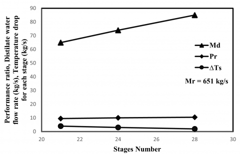
Three modules of 21, 24 and 28 stages plants are tested and the effect of them on the performance ratio, Md and ∆Ts is shown in Figure 1. The results showed that the increase in the stages number increases the performance ratio and the distillate water flow rate while reducing ∆Ts. Also, the increase in stages number increases the capital cost and energy demand.
Figure 1 shows that the specific flow rate of distilled water increases with the increase in the number of the stages (n), while the performance ratio slightly increases with an increment in n. According to this, the distilled water flow rate increases leading to an improvement in the Pr of the system, and the main factor that has a slight impact on the gain of the system. Md increases by 14.7% as the stage number increases from 21 to 24, and by 17.4% as the stage number increases from 24 to 28. While the Pr increment with increasing stage number from 21-24 stages is in the range of 13.4% and 4.5 for stages from 24 to 28 stages. So the preferable system has 24 stages with distilled water up to 73.36 kg/s and Pr in the range of 10. The drop of the temperature is not noticeably affected by the increases of n.
Figure 1. The effect of the stages number on the performance ratio, Md and ∆Ts
3.2.2 The effect of feed seawater flow rate
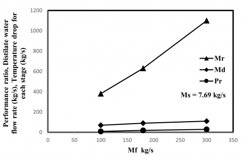
Three amounts of feed seawater flow rate (Mf) are tested and the effect of them on the performance ratio, Md and Mr values are shown in Figure 2. The results showed that the increase of Mf amount increases the performance ratio, recycled flow rate, and the distillate water flow rate. Also, the capital cost and energy demand will increase the heat transfer area.
Figure 2. The effect of the feed flow rate on the performance ratio, Md, and Mr
3.2.3 The effect of heating steam flow rate
As the flow rate of the streams crosses the flashing stages as shown in Figure 2, the brine recycle flow rate (Mr) depends only on the total flashing range (Md), which is independent of the number of stages, as noted in Table 3. While an increase in n causes a decrease in the feed flow of seawater, an increase in the system's thermal performance ratio, Pr, causes a decrease in the feed flow of seawater. Increase of the Pr reduces the heat load which required in the brine heater unit and consequently the quantity of heat removed by the brine recycle flow rate.
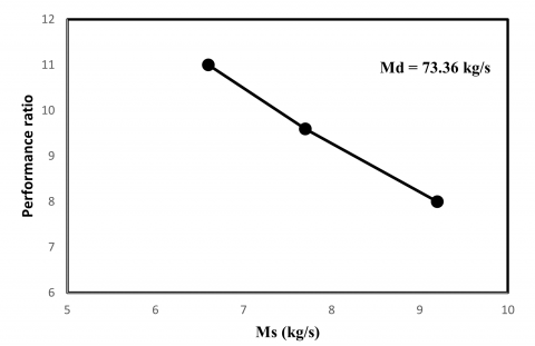
Figure 3. The effect of the heating steam flow rate on the performance ratio
Three different amounts of heating steam flow rate (Ms) are tested, and the effect of each on the performance ratio is shown in Figure 3. The results revealed that increasing Ms increases the performance ratio, capital cost, and energy demand.
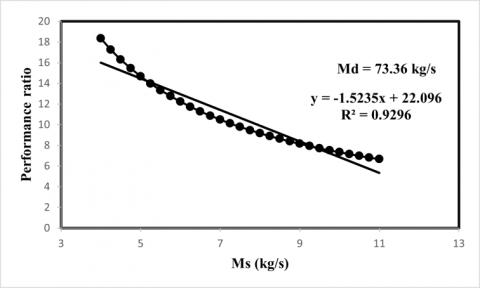
The energy of the steam is consumed to heat the recycle brine Mr to top brine temperature T0 that passes through the first stage. As illustrated in Figure 3, the performance of the system decreases upon an increase in the specific flow rate of the steam Ms in the section of brine heater at constant specific distillate produced across the flashing stages according to Eq. (14). The relation between Pr and Ms is linear if the Ms in the range of 5 – 8 kg/s, while being out of this range the behavior of that relation will be non-linear. In addition, as indicated in Figure 3, the initial interval has a reduction in the system's gain of approximately 24%, but the second interval of Ms rising has a decrement of 3.14% of Pr. That implies the steam flow rate in the heater brine section must be less than 7 kg/s to maintain a high-performance overall system.
Figure 4. The configuration of MSF-M plant design with the main critical parameters
The multistage flash mixing brine distillation plant with 5 MW power is designed to produce about 74 Kg/s of freshwater which is planned to serve Ababa's residents. The plant performance ratio is 9.6 and the design is shown in Figure 4. The feed seawater flow rate, temperature, and salinity are 178 Kg/s, 18℃, and 41000 ppm, respectively. As shown in Figure 4, the plant has 24 stages, each stage has 3.6 m width and 2.6 m length. The brine heater and condenser heat transfer area are 170 m2 and 1626 m2, respectively. The recycled brine characteristics are 651 Kg/s flow rate, 62066 ppm salt concentration, 34℃ temperature, and 110℃ top brine temperature. The brine flow with 40℃ and 70000 ppm salt concentration is rejected to prevent calcium sulfate scaling. The portion of brine flow with 70000 ppm salinity will be discharged to prevent calcium sulfate scaling. The other portion will be recycled to reduce the effect of high salinity and high-temperature flow on the aquatic life and to reduce the energy demand and the cost. Modeling of MSF-M system showed that the operation temperature of the last stage oppositely affects the dimensions of the stage. The heating steam temperature and flow rates are 160℃ and 7.7 Kg/s, respectively.
The effective parameters of MSF-M desalination plant were investigated. The modeling result show that control of the feed seawater temperature is an essential characteristic in the MSF-M process. This is obtained in the mixing tank and in the section of heat rejection of the MSF-M system. Also, it is noted that as the brine temperature in the last stage reduces, which is associated with a great increment in the pressure drop across the stages; it necessitates an extension in the dimensions of the stage to accommodate the sharp development of the vapor-specific volume. These results match with results obtained by modeling the MSF- Brine recirculation MSF-BR) in the study implemented by Manesh [21]. The temperature drop per stage is low at 2.91℃, which increases the temperature driving force for heat transfer and results in a decrease in the heat transfer area of tubes of the preheater/condenser, which agrees with what was reported by Alrawashde [24], Hanshik et al., [23], Gao et al. [12] and Said et al. [20].
In actual operation, the MSF-M system with brine circulation would be preferred, during the winter period. This leads to reducing the quantity of seawater intake and the quantity of chemicals used to control foaming, scaling [23], and corrosion, this matches with results noted by Khashogoftar Manesh et al. [9].
The thermal performance ratio (Pr) declines gradually, and it is necessary to enable the system to run at thermal Pr below 7, where full closedown takes place and cleaning by acid and mechanically might be necessary to recover the unit features to the initial design statuses.
An increase of the salinity in the first stage would cause critical operational problems, because of improved rates of formation for scale and fouling in the tubes of preheater/condenser which cross the stage close to the heater of the brine [23]. Also, leads to an increase in the thermodynamic losses because of the boiling point elevation. That was noted with the MSF- BR system which was modeled by Alrawashdeh et al. [24].
Finally, three main parameters, including the number of stages, heating steam, and feed seawater flow rate are affected the design selection and the performance ratio. As shown in Figures 1, 2 and 3, the design of the plant with 24 stages, 178 Kg/s feed flow rate, and 7.7 Kg/s heating steam flow rate is the most appropriate and cost-effective design. The increase in stages number leads to an increase in the salinity and reduces the temperature through the stages which leads to a partial decrease of specific heat capacity [22]. The capital cost and energy demand increase when the stage number, feed, and steam flow rate increase. On the other hand, the decrease in plant stage number, feed, and steam flow rate will affect plant performance and efficiency.
The MSF-M desalination plant is designed to be supplied by 5 MW power. The designed MSF-M distillation plant has 24 flashing stages with a width of 3.6 m and a length of 2.6 m. The plant performance is 9.6 and freshwater production is 74 Kg/s. Through the operation of this plant, the red sea salinity will increase from 41000 ppm to the maximum allowable value of 70000 ppm in the discharge point. The design of the plant with 24 stages, 178 Kg/s feed flow rate, and 7.7 Kg/s heating steam flow rate is the most appropriate and cost-effective design. The results showed that the gate height increased through the stages from 0.176 m to 0.594 m while the brine pool height increased from 0.376 m to 0.794 m for the first and last stages, respectively. Furthermore, the brine heater and condenser have specific heat transfer areas of 2.295 m2/(Kg/s) and 22 m2/(Kg/s), respectively.
The effective parameters of MSF-M desalination plant were investigated; the modeling results show that the reduction in the brine temperature requires an expansion in the dimensions of the stages. Also, the increment in the salinity causes an incensement of the thermal load. Moreover, the mixing brine technique in order to preheat feed seawater supported the maximization of the system’s performance.
Reductions which are associated with a great increment of the pressure drop across the stages; it necessitates an extension in the dimensions of the stage to accommodate the sharp development of the vapor-specific volume.
Based on the obtained results, the following points could be recommended:
|
Mf |
Feed seawater, kg.s-1 |
|
Cp |
specific heat, J. kg-1. K-1 |
|
Md |
Distillated water, kg.s-1 |
|
X |
Salt concentration, ppm |
|
ʎv |
Vapor enthalpy, kJ.s-1 |
|
Vb |
Brine heater, m.s-1 |
|
ρv |
Vapor density, kg. m-3 |
|
U |
Overall heat transfer coefficient, w.m-2. ℃-1 |
|
Ts |
Steam temperature, ℃ |
|
Tn |
Blow down temperature, ℃ |
|
LMTD |
Logarithmic mean temperature difference, ℃ |
|
BPE |
Boiling point elevation, ℃ |
|
NEA |
Non-equilibrium allowance |
|
A |
Heat transfer temperature, m2 |
|
∆Td |
Temperature drop in demister, ℃ |
|
GH |
Gate height, m |
|
H |
Brine height, m |
|
W |
Width, m |
|
Cd |
Weir fraction coefficient |
|
Subscripts |
|
|
b |
brine |
|
v |
vapor |
|
I |
stage number |
|
s |
steam |
[1] World Bank Group. (2016). Hashemite Kingdom of Jordan Promoting Poverty Reduction and Shared Prosperity: Systmetic Country Diagnostic. World Bank, Washington, DC. https://openknowledge.worldbank.org/handle/10986/23956.
[2] Ministry of Water and Irrigation. (2016). National Water Strategy 2016 - 2025. Jordan. https://www.liportal.de/fileadmin/user_upload/oeffentlich/Jordanien/10_ueberblick/National_Water_Strategy__2016-2025_-25.2.2016.pdf
[3] Elimelech, M., Phillip, W.R. (2011). The future of seawater desalination: Energy, technology, and the environment. Science., 333(6043): 712-717. https://doi.org/10.1126/science.1200488.
[4] Soni, A., Stagner, J.A., Ting, D.S.K. (2017). Adaptable wind/solar powered hybrid system for household wastewater treatment. Sustainable Energy Technologies and Assessments, 24: 8-18. https://doi.org/10.1016/j.seta.2017.02.015
[5] Khawaji, A.D., Kutubkhanah, I.K., Wie, J.M. (2008). Advances in seawater desalination technologies. Desalination, 221(1-3): 47-69. https://doi.org/10.1016/j.desal.2007.01.067
[6] Zhu, Z., Peng, D., Wang, H. (2019). Seawater desalination in China: An overview. Journal of Water Reuse and Desalination, 9(2): 115-132. https://doi.org/10.2166/wrd.2018.034
[7] Navarro, T. (2018). Water reuse and desalination in Spain–challenges and opportunities. Journal of Water Reuse and Desalination, 8(2): 153-168. https://doi.org/10.2166/wrd.2018.043
[8] Krishna, H.J. (2004). Introduction to desalination technologies. Texas Water Dev, 2, 1-7.
[9] Khoshgoftar Manesh, M.H., Kabiri, S., Yazdi, M., Petrakopoulou, F. (2020). Thermodynamic evaluation of a combined-cycle power plant with MSF and MED desalination. Journal of Water Reuse and Desalination, 10(2): 146-157. https://doi.org/10.2166/wrd.2020.025
[10] Raluy, G., Serra, L., Uche, J. (2006). Life cycle assessment of MSF, MED and RO desalination technologies. Energy, 31(13): 2361-2372. https://doi.org/10.1016/j.energy.2006.02.005.
[11] Catrini, P., Cipollina, A., Giorgio, G., Giacalone, F., Micale, G., Piacentino, A., Tamburini, A. (2018). Chapter 12 - Thermodynamic, Exergy, and Thermoeconomic analysis of Multiple Effect Distillation Processes. Renewable Energy Powered Desalination Handbook, Butterworth-Heinemann, 445-489. https://doi.org/10.1016/j.energy.2006.02.005
[12] Gao, H., Jiang, A., Huang, Q., Xia, Y., Gao, F., Wang, J. (2020). Mode-based analysis and optimal operation of MSF desalination system. Processes, 8(7): 794. https://doi.org/10.3390/pr8070794
[13] El-Dessouky, H., Ettouney, H., Al-Juwayhel, F., Al-Fulaij, H. (2004). Analysis of multistage flash desalination flashing chambers. Chemical Engineering Research and Design, 82(8): 967-978. https://doi.org/10.1205/0263876041580668
[14] El-Ghonemy, A.M.K. (2018). Performance test of a sea water multi-stage flash distillation plant: Case study. Alexandria engineering journal, 57(4): 2401-2413. https://doi.org/10.1016/j.aej.2017.08.019
[15] Bodalal, A.S., Abdul_Mounem, S.A., Salama, H.S. (2010). Dynamic modeling and simulation of MSF desalination plants. JJMIE, 4(3): 394-403. http://jjmie.hu.edu.jo/files/v4n3/37-09%20done.pdf
[16] Said, S.A. (2012). MSF process modelling, simulation and optimisation: Impact of noncondensable gases and fouling factor on design and operation. Doctoral dissertation, University of Bradford, Yorkshire, UK. http://hdl.handle.net/10454/5721
[17] El-Dessouky, H.T., Ettouney, H.M. (2002). Fundamentals of Salt Water Desalination. Elsevier. Hamilton, Ontario.
[18] Abduljawad, M., Ezzeghni, U. (2010). Optimization of Tajoura MSF desalination plant. Desalination, 254(1-3): 23-28. https://doi.org/10.1016/j.desal.2009.12.019
[19] Mabrouk, A.N., Fath, H.E. (2015). Technoeconomic study of a novel integrated thermal MSF–MED desalination technology. Desalination, 371: 115-125. https://doi.org/10.1016/j.desal.2015.05.025
[20] Said, S.A., Emtir, M., Mujtaba, I.M. (2013). Flexible design and operation of multi-stage flash (MSF) desalination process subject to variable fouling and variable freshwater demand. Processes, 1(3): 279-295. https://doi.org/10.3390/pr1030279
[21] Manesh, M.H., Kabiri, S., Yazdi, M., Petrakopoulou, F. (2020). Exergoeconomic modeling and evaluation of a combined-cycle plant with MSF and MED desalination. Journal of Water Reuse and Desalination, 10(2): 158-172. https://doi.org/10.2166/wrd.2020.074
[22] Gambier, A., Badreddin, E. (2005). Dynamic modeling of a single-stage MSF plant for advanced control purposes. In Proceedings of 2005 IEEE Conference on Control Applications, 2005. CCA 2005: 681-686. https://doi.org/10.1109/CCA.2005.1507206
[23] Hanshik, C., Jeong, H., Jeong, K.W., Choi, S.H. (2016). Improved productivity of the MSF (multi-stage flashing) desalination plant by increasing the TBT (top brine temperature). Energy, 107: 683-692. https://doi.org/10.1016/j.energy.2016.04.028
[24] Alrawashde, K.A., Talat, N., Alshorman, A. (2017). Multi stage flashing small scale plant combined CHP plant driven by biogas plant. International Journal of Applied, 7(3): 51-59.
[25] Hassanean, M., Nafey, A., El-Maghraby, R., Ayyad, F. (2019). Simulation of multi-stage flash with brine circulating desalination plant. Journal of Petroleum and Mining Engineering, 21(1): 34-42. https://doi.org/10.21608/jpme.2020.73173
[26] Gao, H., Jiang, A., Huang, Q., Xia, Y., Gao, F., Wang, J. (2020). Mode-based analysis and optimal operation of MSF desalination system. Processes, 8(7): 794. https://doi.org/10.3390/pr8070794
[27] Alsehli, M., Choi, J.K., Aljuhan, M. (2017). A novel design for a solar powered multistage flash desalination. Solar Energy, 153: 348-359. https://doi.org/10.1016/j.solener.2017.05.082
[28] Al-Othman, A., Tawalbeh, M., Assad, M.E.H., Alkayyali, T., Eisa, A. (2018). Novel multi-stage flash (MSF) desalination plant driven by parabolic trough collectors and a solar pond: A simulation study in UAE. Desalination, 443: 237-244. https://doi.org/10.1016/j.desal.2018.06.005
[29] Al Ghamdi, A., Mustafa, I. (2016). Exergy analysis of a MSF desalination plant in Yanbu, Saudi Arabia. Desalination, 399: 148-158. https://doi.org/10.1016/j.desal.2016.08.020
[30] Buros, O.K. (2000). The ABCs of Desalting; International Desalination Association: Topsfield, MA, USA.
[31] El-ghonemy, A.M. et al. (2018). Performance test of a sea water multi-stage flash distillation plant: Case study. Alexandria Engineering Journal, 57(4): 2401-2413. https://doi.org/10.1016/J.AEJ.2017.08.019
[32] Al-Karaghouli, A., Kazmerski, L.L. (2013). Energy consumption and water production cost of conventional and renewable-energy-powered desalination processes. Renewable and Sustainable Energy Reviews, 24: 343-356. https://doi.org/10.1016/j.rser.2012.12.064
[33] Mistry, K.H., McGovern, R.K., Thiel, G.P., Summers, E.K., Zubair, S.M., Lienhard, J.H. (2011). Entropy generation analysis of desalination technologies. Entropy, 13(10): 1829-1864. https://doi.org/10.3390/e13101829
[34] Khorshidi, J., Pour, N.S., Zarei, T. (2019). Exergy analysis and optimization of multi-effect distillation with thermal vapor compression system of bandar abbas thermal power plant using genetic algorithm. Iranian Journal of Science and Technology, Transactions of Mechanical Engineering, 43(1): 13-24. https://doi.org/10.1007/s40997-017-0136-7
[35] Cerci, Y. (2002). The minimum work requirement for distillation processes. Exergy, An International Journal, 2(1): 15-23. https://doi.org/10.1016/S1164-0235(01)00036-X
[36] Cerci, Y. (2002). Exergy analysis of a reverse osmosis desalination plant in California. Desalination, 142(3): 257-266. https://doi.org/10.1016/S0011-9164(02)00207-2
[37] Piacentino, A. (2015). Application of advanced thermodynamics, thermoeconomics and exergy costing to a Multiple Effect Distillation plant: In-depth analysis of cost formation process. Desalination, 371: 88-103. https://doi.org/10.1016/j.desal.2015.06.008
[38] El-Dessouky H.T., Ettouney H. (1999). Multiple-effect evaporation desalination systems. Thermal Analysis, Desalination, 125(1-3): 259-276. https://doi.org/10.1016/S0011 9164(99)00147-2
[39] El-Dessouky, H.T., Ettouney, H.M., Al-Roumi, Y. (1999). Multi-stage flash desalination: present and future outlook. Chemical Engineering Journal, 73(2): 173-190. https://doi.org/10.1016/S1385-8947(99)00035-2
[40] Mussati, S., Aguirre, P., Scenna, N.J. (2001). Optimal MSF plant design. Desalination, 138(1-3): 341-347. https://doi.org/10.1016/S0011-9164(01)00283-1
[41] Lappalainen, J., Korvola, T., Alopaeus, V. (2017). Modelling and dynamic simulation of a large MSF plant using local phase equilibrium and simultaneous mass, momentum, and energy solver. Computers & Chemical Engineering, 97: 242-258. https://doi.org/10.1016/j.compchemeng.2016.11.039
[42] Alhazmy, M.M. (2011). Multi stage flash desalination plant with brine–feed mixing and cooling. Energy, 36(8): 5225-5232. https://doi.org/10.1016/j.energy.2011.06.024
[43] Alhazmy, M.M. (2014). Economic and thermal feasibility of multi stage flash desalination plant with brine–feed mixing and cooling. Energy, 76: 1029-1035. https://doi.org/10.1016/j.energy.2014.09.022
[44] Za'al AL-Mahasneh, E., Al-Habees, M.A., Al-Khaddam, H.K. (2012). Urban population growth trends in Jordan (2014-2044). International Journal of Scientific and Engineering Research., 3(10): 1-25. https://www.ijser.org/onlineResearchPaperViewer.aspx?Urban-Population-Growth-Trends-in-Jordan-2014-2044.pdf.
[45] Kotb, O.A. (2015). Optimum numerical approach of a MSF desalination plant to be supplied by a new specific 650 MW power plant located on the Red Sea in Egypt. Ain Shams Engineering Journal, 6(1): 257-265. https://doi.org/10.1016/j.asej.2014.09.001
[46] Chapter 6 Multi-stage Flash Desalination. https://www.coursehero.com/file/10223245/Multi-stage-Flash-Desalination/.
[47] Huddar, D., Holikar, A., Mandhare, A., Jaiswal, S., Bhopale, N.N. (2017). Design of multi-stage flash process as desalination and power generation plant. Vishwakarma Journal of Engineering Research, 1(3): 12-21.
[48] Al-Sofi, M.A.K. (1999). Fouling phenomena in multi stage flash (MSF) distillers. Desalination, 126(1-3): 61-76. https://doi.org/10.1016/S0011-9164(99)00155-1
[49] Attia, S.I. (2015). The influence of condenser cooling water temperature on the thermal efficiency of a nuclear power plant. Annals of Nuclear Energy, 80: 371-378. https://doi.org/10.1016/j.anucene.2015.02.023