S. Vinoth John Prakash | P.K. Dhal*
© 2021 IIETA. This article is published by IIETA and is licensed under the CC BY 4.0 license (http://creativecommons.org/licenses/by/4.0/).
OPEN ACCESS
The output of wind and the solar system is not constant; it is difficult to access the adequacy of the system. The Generation model is developed for 240 MW of different generation units in the Roy Billinton Test System (RBTS). Then a multi-state wind and solar generation model is developed based on different solar radiation and wind speed to evaluate the probability of the states. In this work, the wind and solar systems are studies for separate locations with each consist of 8 MW, 18 MW, 28 MW, and 38 MW generation capacities. This wind and solar generation model are applied to Roy Billinton Test System (RBTS) to evaluate the reliability indices like Loss of Load Expectation (LOLE). Based on the development of the MATLAB program for determining reliability indices, the capacity outage probability is developed for multiple solar and wind states. Based on standard load forecasting and the Time Series Load forecasting technique, the reliability of the system is analyzed. The results reveal the variation of risk indices in the system when additional generators are incorporated into the RBTS generation system. The cost optimization for Solar and Wind system were conducted using HOMER software to obtain the levelized cost of the proposed system.
reliability, cost optimization, loss of load expectation, Roy Billinton test system, solar and wind
1.1 Motivation
Green energies like solar and wind power generation give clean power generation to the environment. The output of renewable energies like Solar and Wind are not constant in nature due to changes in environmental conditions. Due to an outage in the renewable system, there will be a certain level of risk indices. The main motivation of this research is to analyze the risk indices of the renewable energy system incorporated with the RBTS test system and cost optimization. Solar radiation and wind speed are the main parameters for Forced outage Rate. By adding suitable generators, the system will meet the future load demand.
1.2 Literature survey
Gami et al. [1] investigated that the capacity value is used to calculate the utilization of the generator at a given time. Kumar et al. [2] have contributed to the work on Hybrid System Reliability Analysis, Reducing Peak Demand to Boost Reliability, Annual Reliability Efficiency, Systematic Approach to Reliability Studies, Power Management Algorithm, Demand Side Management, Markov Model Reliability Evaluation, Wind Energy Conversion System Uncertainty. For the above works, various methods of evaluation have been considered. These methods are condition monitoring system, column and limitation generation algorithm, analytical procedure, Markov modeling. Reliability enhanced by incorporating the solar and wind systems into the electrical power system was addressed in Refs. [3-7]. Peyghami et al. [8] has addressed the numerous problems in future power systems. Adequateness is the key concern that focuses on this study. The issue typically occurred due to a load demand mismatch in the system. The location of the power plant is also necessary to have an appropriate environmental effect on the production of electricity. A separate mechanism for evaluating the adequacy of the system has been developed. Douglas et al. [9] assessed the risk due to the load forecast uncertainty, during short-term generation planning studies. This forecast depends mainly on the variance. In generation system planning studies, the uncertainty of the load forecast is a crucial factor in the determination of the different reliability indices. As a result, Billinton and Huang [10] discussed the impact of the load forecast uncertainty on the reliability assessment. El-Sheikhi and Billinton [11] investigated the field of load forecast uncertainty, incorporating the assessment of the adequacy of various generator systems, such as Solar and Wind units. Singh et al. [12] explores various forecasting strategies. Various techniques include iterative reweighting of the least square technique, regression technique, multiple regression techniques, and exponential smoothing technique. To predict future loads, the generation of system planners to model load forecasting techniques. Allahnoori et al. [13] is examined that the reliability studies, which may be carried out by considering the load uncertainty. Because the load level has changed every time it is important to predict the load. The authors in references [14-16] addressed the reliability of renewable systems such as solar and wind. This review helps to explain the process of evaluating the system's reliability. Arabali et al. [17] is analyzed that the percentage change in load and it is an assessed the impact on the reliability of the solar / wind system. The load shifting method was carried out to reduce the mismatch between load demand and generation. There are several kinds of research carried out in conducting a multi-state model for both Solar and Wind system [18, 19].
The several research practices for wind and the solar system are to reduce the cost of the system, to improve the reliability, Size Optimization, to reduce the losses, to improve efficiency, etc. [20-23]. These researches are currently active and the researchers are trying to improve the level of the existing system using several techniques. There will be a better result if the freely available natural resources like solar radiation and wind speed are utilized properly. These resources can’t be utilized properly when the solar panels are placed in such a way that the shading occurs due to building near the solar panels and when the wind farm is located where there is less average wind speed according to the last 20 years average wind speed. The solar can be utilized most probably every day due to daily solar radiation but wind can be effectively utilized when there is seasonal wind in Ref. [24]. Nowadays for solar panels, tree type model has been developed to save space in the environment [25]. So, by using this tree model it can fix different solar panels in small space. The reliability in the solar and wind system will be improved by appropriately utilizing the resource [26, 27]. The solar radiation and wind speed data was accessed and collected for evaluating forced outage rate [28]. Ali Kadhem et al. [29] highlights the contribution of integrating wind generators to the RBTS system. The reliability indices like Loss of Load Expectation are evaluated. The LOLE is 1.115 hrs/year when 53 numbers of 0.035 MW added to the RBTS system and LOLE is 0.987 hrs/year when 106 numbers of 0.035MW added to the RBTS system. Sulaeman et al. [30] highlighted the reliability of the RBTS and the IEEE test system integrated Solar PV system. When 30 MW solar PV added to RBTS system, then the Loss of Load Expectation (LOLE) is 0.69888 hrs/year. When 30 MW solar PV added to IEEE test system, then the Loss of Load Expectation (LOLE) is 8.5613 hrs/year. Lalitha et al. [31] discussed reliability indices Loss of Load Expectation (LOLE) for RBTS integrated Wind system. When a 30 MW wind farm added to the RBTS system, then the Loss of Load Expectation (LOLE) is 1.5627 hrs/year. Prasad et al. [32] discusses the adequacy assessment of the system. The LOLE for the system is 1.09845 hrs/year. Roy et al. [33] discusses the reliability assessment model for the wind system. The LOLE for varies from 0.2 hrs/year to 0.4 hrs/year when 30 MW and 90 MW wind power added to the RBTS system with peak load varied from 185 MW to 195 MW. Jiang et al. [34] highlights the reliability of the wind farm. The Loss of Load Expectation (LOLE) for RBTS integrated Wind system is 0.7895 hrs/year. The authors in references [35-38] analyzed the cost of Solar/Wind can be optimized based on the net cost of the system. The system can be modeled with different components to have an optimum value.
1.3 Contributions proposed in the paper
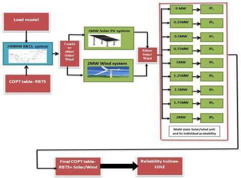
Since the wind and Solar system will not be available every time, the Forced Outage Rate (FOR) is an important factor to evaluate during system analysis. After knowing the FOR value of wind and the solar unit, the Capacity Outage Probability Table (COPT) has developed based on the proposed methodology of adequacy assessment. Then the 185 MW load duration Curve is drawn from the RBTS load data. Then the 240 MW RBTS test system is added to 8 MW, 18 MW, 28 MW, 38 MW solar/wind unit with different FOR values. Each unit consist of 2 MW then this is subdivided in to 0 MW, 0.25 MW, 0.5 MW, 0.75 MW, 1 MW, 1.25 MW, 1.5 MW, 1.75 MW, 2 MW as 9 states. Then the individual probability is evaluated for every case. The hourly load duration curve will start from 0 hrs to 8760 hrs. Then the reliability indices like Loss of Load Expectation (LOLE) of the system is calculated based on individual probability IPi and time Ti values. The cost optimization performed for Solar and Wind system.
The objective function is:
Minimize cost of the system $=\sum_{n}\left(C_{c a, a n n}+C_{r e, a n n}+C_{o m, a n n}\right)$
where, n is different components in the system like Solar Photovoltaic panels, Wind turbine, converter and battery, Cca,ann is annual Capital cost, Cre,ann is Annual replacement cost, Com,ann is Annual Operation and Maintenance cost.
Then the reliability of the system evaluated based on load forecasting technique. The amount of solar/wind power that can’t able to supply power to the load is known as Loss of Load Expectation. The Loss of Load Expectation can be calculated in Eq. (1).
$L O L E=\sum_{i=1}^{n}[I P i * t i] *(365 / 100)$ (1)
where,
IPi- Individual Probability of ith unit.
ti- Time in % for Load duration curve.
The generation system is adequate to meet the future load demand referred to as adequacy assessment. The overall methodology for adequacy assessment of solar and wind incorporated Roy Billinton Test System (RBTS) is shown in Figure 1. The Capacity Outage Probability Table is important to understand the probability of different states. Based on the outages in each state, the Individual Probability (IPi) is evaluated. Renewable energies like solar and wind are considered in this study as 2 MW for 1 unit. This one unit is categorized into 9 states since the Solar and Wind is changing every time due to it depends on the environmental condition. The solar radiation and wind speed are not constant every time but it was intermediate. The wind turbine blades will be damaged when the speed of the wind increases to 25 m/s. During this time, the wind turbine is allowed to stop using some braking action. The hourly solar radiation is observed for a particular location to evaluate the output power of the solar system. The load is modeled based on standard load forecasting and time series load forecasting techniques. For 9 years, the reliability indices are calculated. The load data is identified based on load modeling. Initially, the 185 MW Roy Billinton Test System (RBTS) load duration curve is drawn to determine the risk indices of the system [10]. According to the result of this load data, the reliability is evaluated based on the generation system. Based on the Individual Probability (IPi) and the time correspond to a capacity outage, the reliability like Loss of Load Expectation is evaluated. The LOLE is represented in days/year. The generation model of RBTS generation system, solar and wind system is discussed in section 4. The solar/wind model is incorporated with the RBTS system to enhance the result of system reliability indices. In this study, a minimum of 8 MW is added to the RBTS system initially. Then an additional 10 MW is added up to 38 MW to satisfy the future load demand. The MATLAB program has been written to evaluate the Individual Probability (IPi) of each generation state in the Capacity Outage Probability Table. The Individual Probability (IPi) depends on the unavailability, availability of the generation system, and the number of units and number of units on forced outages. Mathematically, the Individual Probability (IPi) is shown in Eq. (2).
$I P i=\frac{N !}{F O !(N-F O) !} W^{f} . Y^{N-F O}$ (2)
where, W = Unavailability, Y = Availability, FO = No of units on the forced outage, N = No of units.
Figure 1. Methodology for adequacy assessment
4.1 Generation model
In this section, the Roy Billinton Test System generation model and solar/wind generation model were discussed.
4.1.1 Roy Billinton Test System Generation model
The Roy Billinton Test System (RBTS) consist of two 5MW hydro generation units with FOR as 0.010 each, four 20MW hydro generation units with each 0.015 FOR each, one 20MW thermal generation units with 0.025 FOR, one 40MW hydro generation units with 0.020 FOR, two 40MW thermal generation unit with 0.030 FOR each, one 10MW thermal generation unit with FOR 0.020. There are a total of 11 generation units available in the RBTS test system. Based on the unavailability ‘W’ of each generation unit, the Individual Probability ‘IPi’ is evaluated. Then the Capacity Outage Probability Table developed for the RBTS generation system based on the methodology of adequacy assessment. Each state consists of 5MW, so a total of 49 states are evaluated in the COPT table to evaluate the expected loss of load. The Roy Billinton Test system representing the generation units is shown in Figure 2.
Figure 2. RBTS generation system
4.1.2 Mathematical modeling of solar and wind generation
Solar radiation is an important parameter for evaluating solar output power. The Solar output power ‘PS’ is evaluated using the Eq. (3).
Solar output power PS = ηS * SN * SA * SR (3)
where, SR= Average solar radiation, SA = Area of solar (m2), SN = Number of solar panels, ηS = Efficiency of the solar panel. The wind speed data is an important factor
The Wind output power ‘PWT’ is evaluated using the Eq. (4).
$P_{W T}=\left\{\begin{array}{lr}0 & 0 \leq w<w s c i \\ \operatorname{Pr} *(E+F * v+G * v * v) & w c i \leq w<w r \\ \operatorname{Pr} & w r \leq w<w c o \\ 0 & w \geq w c o\end{array}\right.$ (4)
where, w = wind speed (m/s), wci - Cut in wind speed (m/s), wco = Cut out wind speed (m/s), wr = Rated wind speed (m/s), Pr = Rated output power (MW), E,F,G = calculated from a cut in, cut out and rated wind speed.
Based on the output power of wind and solar PV systems, the Forced Outage Rate is calculated. The Forced outage Rate is 0.756 for solar and 0.749 for wind.
4.2 Load modeling
The Load is modeling based on standard load forecasting and time series load forecasting techniques. The procedure for this two-forecasting technique for assessing the adequacy is discussed in this section.
4.2.1 Standard load forecasting
In standard load forecasting, an increase in 5% load is assumed to be the future load demand. The 5% load is increased till 2028 from 2020. The load data is collected from the 185 MW RBTS test system for the year 2020 to evaluate the risk indices. The advantages in making Standard Load forecasting is to predict future load data reasonably and accurately. Normally the standard load growth for different location considered as 5%. Due to increasing in industries, residents, commercial loads in a year, the load growth will increase every year. For future years, the corresponding load growth obtained using standard and time-series load forecasting techniques.
4.2.2 Procedure for time-series load forecasting technique
The Time series load forecasting is the technique used for forecasting the load in advance in which the set of load data is recorded for specified interval of time. By using this technique, the future load determined for evaluating future reliability indices. The Procedure for Time-series load forecasting technique as follow:
Step 1: Observe the load demand values at regular time.
Step 2: Determine the Latest load forecasting using in Eq. (5).
LFt= β(PLt-1- PFt-1)+ PFt-1 (5)
where,
PLt-1 = Past load demand,
LFt = Latest forecast,
PFt-1 = Past forecast,
β- Constant (0 ≤ β ≤1).
Step 3: The Error is defined as the difference between actual measurement and forecast for time ‘t’.
Evaluate Error during measurement using Eq. (6).
Error = Ωt- µt (6)
Ωt-= Actual measurement for time period ‘t’.
µt-= Forecast for same time period ‘t’.
Step 4: The percentage error is the ratio of the difference between actual measurement ‘Ωt’ and forecast for the period ‘t’ ‘µt’ and forecast for the period ‘t’. The Error in % is represented in Eq. (7).
$\operatorname{Error} \%=\frac{\Omega t-\mu t}{\mu t}$ (7)
Step 5: The Average error is the average difference between actual measurement ‘Ωt’ and forecast for the period‘t’ ‘µt’. The average error is evaluated in Eq. (8).
Average error $=\frac{1}{\text { number of values }}+\sum_{t=0}^{n}(\Omega t-\mu t)$ (8)
Step 6: The Average square error is the average square of the difference between the actual measurements ‘Ωt’ and forecast for the period ‘t’ ‘µt’. The Average square error is evaluated in Eq. (9).
Average square error $=\frac{1}{\text { number of values }}+\sum_{t=0}^{n}(\Omega t-\mu t)^{2}$ (9)
Step 7: The Root average square error is the square root of average values in the square of the difference between the actual measurement ‘Ωt’ and forecast for the period ‘t’ ‘µt’. The Root Average square error is evaluated using (10).
Root Average square error $=\sqrt{\frac{1}{\text { number of values }}+\sum_{t=0}^{n}(\Omega t-\mu t)^{2}}$ (10)
Step 8: The Mean absolute percentage error is the average of percentage error and it is given in Eq. (11).
Mean Absolute % Error $=\frac{1}{\text { number of values }} \sum_{t=0}^{n} Error \%$ (11)
Step 9: The Standard error deviation is the average square of the difference between the average error and error. It is represented in Eq. (12).
Standard Error Deviation $=\sqrt{\frac{1}{\text { number of values }}+\sum_{t=0}^{n} \text { (Average error - error) }^{2}}$ (12)
5.1 Error measurement analysis
The error is measured during the process of time series load forecasting. The load can be predicted in advance for several years. The absolute error measurement, Root Average Square Error, Maximum negative error, Maximum positive error is discussed in this section.
5.1.1 Measurement of error (absolute)
The error is measured during the processing of data. The value is measured and it is represented by ‘Xm’. The value which is already known was represented by ‘XK’. Then the difference between Xm and XK is known as Absolute error measurement. Based on the procedure of the time series load forecasting technique, the results are obtained as shown in Table 1. The maximum positive and negative error is 0.4 and -0.9. The mean absolute error is determined and it is 0.38. Between two variables when the result is not obtained between these two variables then in correlation measurement there is an error. The correlation obtained is in absolute error measurement is 0.999563. The coefficient of determination is forecasted from the independent variable. The coefficient of determination R2 = 99.8851%. Then the 99.8851% of the dependent variable variability is taken into account and 0.1149% of the residual variability is now undercounted.
Table 1. Measurement of error (absolute)
|
Post Processed result |
Model fit |
|
Number of Observations |
5 |
|
Maximum negative error |
-0.9 |
|
Maximum positive error |
0.4 |
|
Mean absolute error |
0.38 |
|
Root average square error |
0.479583 |
|
Residual sum |
-0.5 |
|
The standard deviation of residuals |
0.469042 |
|
Coefficient of determination (R2) |
0.998851 |
|
Correlation |
0.999563 |
5.1.2 Measurement of error (range %)
Table 2. Measurement of error (range %)
|
Post Processed result |
Model fit |
|
Number of observations |
5 |
|
Maximum negative error |
-2.25% |
|
Maximum positive error |
1% |
|
Normalized average absolute error |
0.95% |
|
Normalized root average square error |
1.19896% |
|
Residual sum |
-1.25% |
|
The standard deviation of residuals |
1.1726% |
|
Coefficient of determination (R2) |
0.998851 |
|
Correlation |
0.999563 |
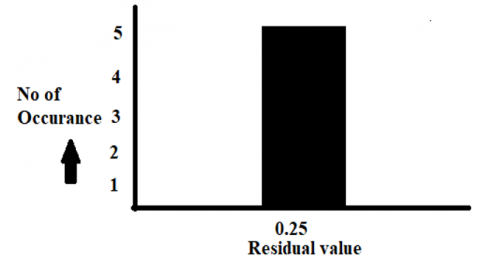
The measurement of error is an important factor for analyzing better results. In the load time series load forecasting, the load was predicted in advance. The load is forecasted based on the previous values. There are different parameters analyzed based on the time series forecasting procedure as shown in Table 2. The maximum positive and negative error is determined as 1% and -2.25%. Then the average absolute error is 0.95%. The disparity between the data and an approximation mode is calculated in the residual sum. The residual sum is estimated as -1.25%. Then the standard deviation of the residuals is evaluated as 1.1726%. The latest forecast is evaluated for 9 years based on the observed value using the time-series load forecasting technique. The number of times an observation occurs in a given load forecast data is referred as number of occurrences. Since residual value determined as 0.25 with 5 number of occurrences, it is considered as final value. The measurement during time- series load forecasting, the residual value is obtained as shown in Figure 3.
Figure 3. Residual value in the measurement
5.1.3 Measurement of error (target %)
Based on the time series forecasting procedure, the error, different parameters are tabulated for measurement as shown in Table 3. There are five observations taken during load forecasting. The variables will be forecasted based on the observed value. There is an error in measurement due to the vast variation in the observed variables. The maximum positive and negative error during model fit is 0.196078% and -0.486486%. Then the root average square percentage error is 0.25%. The Standard deviation of residuals is 0.243475%.
Table 3. Measurement of error (target %)
|
Post processed result |
Model fit |
|
Number of Observations |
5 |
|
Maximum negative error |
-0.486486% |
|
Maximum positive error |
0.196078% |
|
Average absolute % error |
0.191184% |
|
Root average square % error |
0.25% |
|
Residual sum |
-0.0488998% |
|
The standard deviation of residuals |
0.243475% |
|
Coefficient of determination (R2) |
0.998851 |
|
Correlation |
0.999563 |
5.1.4 Evaluation of the latest forecast
The observed load demand for 5 years is taken as a variable to forecast the load. The minimum value of load demand is 185 MW and the maximum value of load demand is 225 MW. Based on this, the median, mean value, and standard deviation are evaluated and shown in Table 4.
Table 4. System load parameters
|
Variable |
System load |
|
Numeric values |
5 |
|
Minimum value |
185 MW |
|
Maximum value |
225 MW |
|
Median |
204 MW |
|
Mean value |
204.5 |
|
Standard deviation |
14.1483 |
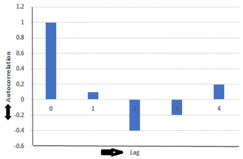
There are different measurements P1 ≤ P ≤ Pn for different time intervals T1 ≤ T≤ Tn. The autocorrelation function is evaluated based on the lag‘f’ from the Eq. (13). Based on this Eq. (13). the autocorrelation curve is represented in Figure 4.
$r=\frac{\sum_{i=1}^{n-f}(\mathrm{Pi}-\mathrm{P})(\mathrm{Pi}+1-\mathrm{P})}{\sum_{i=1}^{n}(\mathrm{Pi}-\mathrm{P})^{2}}$ (13)
Let the time interval ‘T’ is assumed variable so that ‘T’ not evaluated in the above equation.
Figure 4. Autocorrelation in time series load forecasting method
Table 5. Latest forecast result using Time series Load forecasting
|
Year |
Actual |
Latest forecast |
Lower |
Upper |
Residuals |
|
2020 |
185 |
184.1 |
183.14 |
185.05 |
-0.9 |
|
2021 |
194.3 |
194.25 |
193.29 |
195.20 |
4.76916 E-11 |
|
2022 |
204 |
204.4 |
203.44 |
205.35 |
0.4 |
|
2023 |
214.3 |
214.55 |
213.59 |
215.50 |
0.3 |
|
2024 |
225 |
224.7 |
223.74 |
225.65 |
-0.3 |
|
2025 |
- |
234.85 |
233.89 |
235.80 |
- |
|
2026 |
- |
245 |
244.04 |
245.95 |
- |
|
2027 |
- |
255.15 |
254.19 |
256.10 |
- |
|
2028 |
- |
265.3 |
264.34 |
266.25 |
- |
Figure 5. Confidence band reliability analyze of solar and wind
The load demand for the first 5 years between 2020 and 2024 is given as input data. The observed actual data for the first 5 years are 185, 194.3, 204, 214.3, and 225. These values are represented in MW. Based on the observed values, the latest forecast is determined using the time series forecasting technique. There is some deviation in the perdition result compared to the observed value. For each year’s latest forecast, the upper and lower limit is determined. The corresponding residuals for the observed value are highlighted in the result. These latest forecasts are determined using the time series forecasting technique to evaluate the reliability of the system. These predicted values help to determine the reliability of the future system. The results of the latest forecast using the time series forecast technique are shown in Table 5. There is better accuracy in the result which is highlighted as the confidence band shown in Figure 5.
The average solar radiation and wind speed was downloaded from the NASA data available in HOMER software for the particular location. The HOMER software gives the optimal solution and gives the least net present cost of the system. The optimization of cost obtained based on the objective function.
The Annualized cost is the total cost of the system, which includes capital cost, replacement cost and operating cost. This annualized cost can be calculated from Eq. (14).
Cann=QC*[(Cca,ann+Cre,ann)*FCR (IR,YN)]+Com,ann (14)
The Capital Recovery factor FCR is represented in Eq. (15).
FCR(IR,YN)=[IR(1+IR)Yn]/[(1+IR)Yn-1] (15)
where, IR is the annual interest rate in %, YN is the number of years.
The Net present cost is the ratio of annualized total cost of the system to the Lifetime of the project as shown in Eq. (16).
The Net present $\operatorname{Cost}\left(\mathrm{C}_{\mathrm{NP}}\right)=\frac{C_{T, a n n}}{F_{C R}\left(I_{R}, P_{L}\right)}$ (16)
where, $C_{T, a n n}$ is the annualized total cost of the system in \$/year, $T_{L_{n, a n n}}$is the total load served by the system annually.
The annual interest rate is 41.2% and The Project lifetime was taken as 25 years for this study. The annualized total cost of the system is \$ 1,60,352 and the total load consumption is 7,19,188 kWh/year.
7.1 Reliability analysis of solar and wind
The reliability of Solar and wind was analyzed by Standard and Time series load forecasting technique.
7.1.1 Reliability of solar and wind with standard load forecasting technique
The Loss of Load Expectation is one of the reliability indices considered in this study. The standard load forecasting technique is applied to evaluate the load demand in the future.
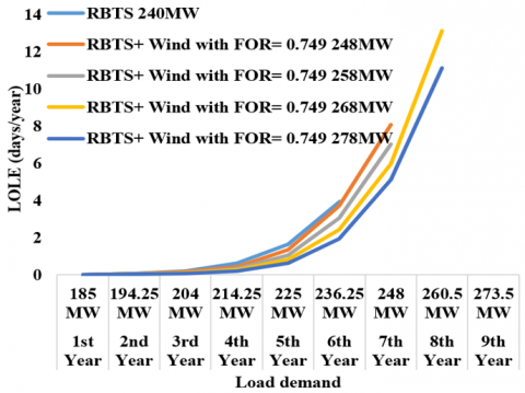
The current RBTS generation system can’t meet the future load demand due to less generation capacity. So, to understand the losses of load that occur on the system, the reliability indices are evaluated based on the methodology of adequacy assessment. The RBTS generation not possible to meet the load after the 7th year due to the load demand is greater than the generation. The solar and wind units were incorporated into the RBTS test system and then the expected loss of load is determined. The Loss of Load Expectation decreases when adding additional solar and wind to RBT generation system. The reliability improved after adding the capacities of solar and wind to the RBTS system. In the 9th year, after adding 38 MW wind and solar, the Loss of Load Expectation is 27.2427 days/year and 27.75952 days/year. The Variation in LOLE indices with RBTS generation system is incorporated into the wind and solar system using standard load forecasting as shown in Tables 6 and 7. The Variation of LOLE and load demand for RBTS is incorporated in the wind and solar system using standard load forecasting, it is graphically represented in Figures 6 and 7.
7.1.2 Reliability of solar and wind with time series load forecasting technique
The Time series load forecasting technique is applied to evaluate the load demand in the future. The load forecasting is done for 9 years based on the procedure of time series load forecasting. This technique is used to evaluate the risk indices in the system. When utilizing only the RBTS generation, then it is not possible to generate power after the 6th year. The various capacities of solar/wind are incorporated into the RBTS system to analyze the reliability indices like Loss of Load.
Expectation. Loss of load expectation is gradually increasing every year. Due to additional capacities like Solar and Wind added to the system, the loss of load expectation decreases. The Variation in LOLE indices with RBTS generation system is incorporated into the wind and solar system using the time series load forecasting technique shown in Tables 8 and 9. The Variation of LOLE and load demand for RBTS is incorporated in the wind and solar system using the time series load forecasting technique is graphically represented in Figures 8 and 9.
Table 6. Variation in LOLE indices with RBTS incorporated to wind system using standard load forecasting
|
Installed capacity |
LOLE (days/year)- Load growth at 5% per year (Forecast peak load) |
|||||||||
|
1st Year |
2nd Year |
3rd Year |
4th Year |
5th Year |
6th Year |
7th Year |
8th Year |
9th Year |
||
|
185 MW |
194.25 MW |
204 MW |
214.25 MW |
225 MW |
236.25 MW |
248 MW |
260.5 MW |
273.5 MW |
||
|
RBTS |
240 MW |
0.026222 |
0.079486 |
0.209181 |
0.613010 |
1.637236 |
3.959987 |
_ |
- |
- |
|
RBTS+ Wind with FOR= 0.749 |
248 MW |
0.021035 |
0.0595370 |
0.156349 |
0.448146 |
1.3626325 |
3.721862 |
8.086882 |
_ |
_ |
|
258 MW |
0.015186 |
0.055428 |
0.120427 |
0.340281 |
1.039402 |
3.067690 |
7.037390 |
_ |
- |
|
|
268 MW |
0.011287 |
0.041197 |
0.095041 |
0.257979 |
0.814372 |
2.417501 |
5.979675 |
13.14533 |
_ |
|
|
278 MW |
0.008321 |
0.025612474 |
0.074967 |
0.204406 |
0.631164 |
1.930171 |
5.107580 |
11.12189 |
27.2427 |
|
Table 7. Variation in LOLE indices with RBTS incorporated to solar system using standard load forecasting
|
Installed capacity |
LOLE (days/year)- Load growth at 5% per year (Forecast peak load) |
|||||||||
|
1st Year |
2nd Year |
3rd Year |
4th Year |
5th Year |
6th Year |
7th Year |
8th Year |
9th Year |
||
|
185 MW |
194.25 MW |
204 MW |
214.25 MW |
225 MW |
236.25 MW |
248 MW |
260.5 MW |
273.5 MW |
||
|
RBTS |
240 MW |
0.026222 |
0.079486 |
0.209181 |
0.613010 |
1.637236 |
3.959987 |
_ |
_ |
_ |
|
RBTS+ Solar with FOR= 0.756 |
248 MW |
0.021178 |
0.059882 |
0.157332 |
0.450795 |
1.370528 |
3.738114 |
8.113198 |
_ |
_ |
|
258 MW |
0.015429 |
0.045430 |
0.121790 |
0.345676 |
1.052739 |
3.101338 |
7.089643 |
_ |
_ |
|
|
268 MW |
0.011576 |
0.034192 |
0.096956 |
0.262966 |
0.831736 |
2.464235 |
6.060183 |
13.32111 |
_ |
|
|
278 MW |
0.008576 |
0.026379 |
0.076888 |
0.209556 |
0.647267 |
1.976308 |
5.195023 |
11.32215 |
27.75952 |
|
Table 8. Variation in LOLE indices with RBTS incorporated to wind system using time series load forecasting
|
Installed capacity |
LOLE (days/year)-Time series load forecasting technique |
|||||||||
|
1st Year |
2nd Year |
3rd Year |
4th Year |
5th Year |
6th Year |
7th Year |
8th Year |
9th Year |
||
|
184.1 MW |
194.25 MW |
204.4 MW |
214.55 MW |
224.7 MW |
234.85 MW |
245 MW |
255.15 MW |
265.3 MW |
||
|
RBTS |
240 MW |
0.02294 |
0.077336 |
0.206535 |
0.59092 |
1.61069 |
3.957268 |
_ |
_ |
_ |
|
RBTS+ Wind with FOR= 0.749 |
248 MW |
0.018604 |
0.059539 |
0.164852 |
0.46017 |
1.328163 |
3.32918 |
6.84083 |
_ |
_ |
|
258 MW |
0.01299 |
0.055429 |
0.131342 |
0.354138 |
1.01409 |
2.665814 |
5.770971 |
11.023565 |
_ |
|
|
268 MW |
0.009307 |
0.041198 |
0.109026 |
0.274199 |
0.792572 |
2.10532 |
4.951535 |
9.100932 |
17.215689 |
|
|
278 MW |
0.006734 |
0.025612 |
0.085242 |
0.216033 |
0.616445 |
1.683172 |
4.099724 |
7.872568 |
15.18512 |
|
Table 9. Variation in LOLE indices with RBTS incorporated to solar system using time series load forecasting
|
Installed capacity |
LOLE (days/year)- Time series load forecasting technique |
|||||||||
|
1st Year |
2nd Year |
3rd Year |
4th Year |
5th Year |
6th Year |
7th Year |
8th Year |
9th Year |
||
|
184.1 MW |
194.25 MW |
204.4 MW |
214.55 MW |
224.7 MW |
234.85 MW |
245 MW |
255.15 MW |
265.3 MW |
||
|
RBTS |
240 MW |
0.023345 |
0.078285 |
0.207535 |
0.59199 |
1.619027 |
3.970817 |
_ |
_ |
_ |
|
RBTS+ Solar with FOR= 0.756 |
248 MW |
0.018652 |
0.059882 |
0.168926 |
0.463024 |
1.336243 |
3.343553 |
6.865008 |
_ |
_ |
|
258 MW |
0.013099 |
0.045432 |
0.133802 |
0.35693 |
1.026625 |
2.699814 |
5.820498 |
11.358987 |
_ |
|
|
268 MW |
0.009437 |
0.034193 |
0.109427 |
0.277017 |
0.809763 |
2.141816 |
5.017673 |
9.21352 |
16.912565 |
|
|
278 MW |
0.006778 |
0.026379 |
0.085242 |
0.218945 |
0.632096 |
1.725497 |
4.184411 |
7.991503 |
15.44692 |
|
Table 10. Net present cost for solar and wind system when multiplier=1
|
Name of system components |
Capital cost (\$) |
Operating cost (\$) |
Replacement cost (\$) |
Salvage |
Total cost (\$) |
|
Flat plate Solar PV |
1,06,904 |
2,303 |
0 |
0 |
1,09,207 |
|
Generic 3 kW Wind |
2,42,667 |
1,56,854 |
0 |
0 |
3,99,521 |
|
1 kWh Lead acid battery |
6,20,400 |
2,67,341 |
8,00,199 |
-1,28,910 |
15,59,030 |
|
Converter |
1,693 |
2,919 |
718.47 |
-135.22 |
5,196 |
|
Total |
9,71,664 |
4,29,417 |
8,00,918 |
-1,29,045 |
20,72,954 |
Figure 6. Variation of LOLE and load demand for RBTS incorporated Wind system using standard load forecasting
Figure 7. Variation of LOLE and load demand for RBTS incorporated Solar system using standard load forecasting
Figure 8. Variation of LOLE and load demand for RBTS incorporated Wind system using Time series load forecasting
Figure 9. Variation of LOLE and load demand for RBTS incorporated Solar system using Time series load forecasting
7.2 Cost optimization results with sensitivity analysis for solar and wind system
The generation system considered is Solar and Wind system. The capacity of Solar PV system is 2494 kW and the capacity of Wind is 546 kW. The total cost i.e. net present cost was analyzed based on the system components used. The Solar and Wind system are operated with converter and battery components. To analyze the system, the residential load was considered as 1971.19 kWh/day with peak load of 139.94 kW. This residential load data is taken from HOMER software to understand the levelized cost and net present cost of the system. The capital cost, replacement cost, operating cost and salvage for Generic 3 kW Wind and Flat plate Solar PV with battery and converter was shown in Table 10. This table describes the net present cost for the system. The levelized cost of Solar and Wind are 0.00229 \$/kWh and 0.0294 \$/kWh.
The multiplier for every component was set to 0.75 and 1. Table 11 shows when the multiplier set to 1. The total Net present cost is \$ 20,72,954. If the multiplier set to 0.75, then the capital and operating cost reduced to 25%. During this case, there was variation in the net present cost and cost of energy.
The Net present cost for this proposed optimization model was reduced from \$ 27,60,000 to \$ 20,72,954. The best solution from several iteration in HOMER software is highlighted in Table 11. The below result shows the best solution of net present cost and levelized cost of energy calculated from various iteration using HOMER software. Similarly, Levelized cost of Energy reduced from \$ 0.296 to \$ 0.223 when multiplier set to 1 and when multiplier set to 0.75 then the levelized cost of Energy \$ 0.167 and the net present cost is \$ 15,50,000. The Table 11 shows the Sensitivity analysis with variation in Capital and operating cost of the system.
Table 11. Sensitivity analysis with variation in capital and operating cost
|
System parameters |
Multiplier=1 |
Multiplier=1 |
Multiplier=0.75 |
|
Base model |
Proposed model |
Proposed model |
|
|
Net Present cost |
\$ 27,60,000 |
\$ 20,72,954 |
\$ 15,50,000 |
|
Levelized cost of Energy (for kWh) |
\$ 0.296 |
\$ 0.223 |
\$ 0.167 |
The reliability and cost are evaluated for the system consists of Solar and Wind. The adequacy is assessed in the system which is analyzed using standard load forecasting and time series load forecasting techniques. There were better reliability and cost of the system in the result of the methodology utilized. In the proposed methodology of adequacy assessment, the reliability indices like Loss of Load Expectation are evaluated. The results show that the RBTS generation system will satisfy the load demand only for 6 years. The solar/wind capacities of 38 MW are embedded in the RBTS system to meet the load demand in the 9th year. So, in this 9th year, the LOLE for wind and solar using standard load forecasting technique is 27.2427 days/year and 27.75952 and using time series load forecasting technique is 15.18512 days/year and 15.44692 days/year. The maximum negative and positive errors during measurement using the time series forecasting method are -0.486486% and 0.196078%. The latest load forecast is evaluated using this method based on the observed load demand. The methodology developed will helps to analyze the reliability of the system for various cases. The cost optimization for Solar and Wind were conducted using HOMER software. The result shows that the Levelized cost is minimized from $ 0.296 to $ 0.223. The main innovation for conducting this research is the reliability evaluated using forecasting technique which can be used for generation planning and cost optimization gives the best solution with less cost for the system.
My sincere thanks to my supervisor, Dr. P.K. Dhal, for his suggestions given for my research work. It is worth mentioning that his guidelines and conceptual ideas at every stage have shaped my work in the right direction.
[1] Gami, D., Sioshansi, R., Denholm, P. (2017). Data challenges in estimating the capacity value of solar photovoltaics. IEEE Journal of Photovoltaics, 7(4): 1065-1073. https://doi.org/10.1109/JPHOTOV.2017.2695328
[2] Kumar, S., Saket, R. K., Dheer, D.K., Holm-Nielsen, J. B., Sanjeevikumar, P. (2020). Reliability enhancement of electrical power system including impacts of renewable energy sources: a comprehensive review. IET Generation, Transmission & Distribution, 14(10): 1799-1815. https://doi.org/10.1049/iet-gtd.2019.1402
[3] Adefarati, T., Bansal, R.C., Justo, J.J. (2017). Reliability and economic evaluation of a microgrid power system. Energy Procedia, 142: 43-48. https://doi.org/10.1016/j.egypro.2017.12.008
[4] Adefarati, T., Bansal, R.C. (2017). Reliability and economic assessment of a microgrid power system with the integration of renewable energy resources. Applied Energy, 206: 911-933. https://doi.org/10.1016/j.apenergy.2017.08.228
[5] Adefarati, T., Bansal, R.C. (2019). Reliability, economic and environmental analysis of a microgrid system in the presence of renewable energy resources. Applied Energy, 236: 1089-1114. https://doi.org/10.1016/j.apenergy.2018.12.050
[6] Adefarati, T., Bansal, R.C. (2017). Reliability assessment of distribution system with the integration of renewable distributed generation. Applied Energy, 185: 158-171. https://doi.org/10.1016/j.apenergy.2016.10.087
[7] Hahn, B., Durstewitz, M., Rohrig, K. (2007). Reliability of wind turbines-Experience of 15 years with 1,500 WTs, wind energy. In Proc. Euromech Colloquium, Springer, Berlin (Vol. 101).
[8] Peyghami, S., Palensky, P., Blaabjerg, F. (2020). An overview on the reliability of modern power electronic based power systems. IEEE Open Journal of Power Electronics, 1: 34-50. https://doi.org/10.1109/OJPEL.2020.2973926
[9] Douglas, A.P., Breipohl, A.M., Lee, F.N., Adapa, R. (1998). Risk due to load forecast uncertainty in short term power system planning. IEEE Transactions on Power Systems, 13(4): 1493-1499. https://doi.org/10.1109/59.736296
[10] Billinton, R., Huang, D. (2008). Effects of load forecast uncertainty on bulk electric system reliability evaluation. IEEE Transactions on Power Systems, 23(2): 418-425. https://doi.org/10.1109/TPWRS.2008.920078
[11] El-Sheikhi, F.A., Billinton, R. (1991). Load forecast uncertainty consideration in generating unit preventive maintenance scheduling for single systems. 1991 Third International Conference on Probabilistic Methods Applied to Electric Power Systems, London, UK, pp. 241-245.
[12] Singh, A.K., Khatoon, S., Muazzam, M., Chaturvedi, D.K. (2012). Load forecasting techniques and methodologies: A review. In 2012 2nd International Conference on Power, Control and Embedded Systems, Allahabad, India, pp. 1-10. https://doi.org/10.1109/ICPCES.2012.6508132
[13] Allahnoori, M., Kazemi, S., Abdi, H., Keyhani, R. (2014). Reliability assessment of distribution systems in presence of microgrids considering uncertainty in generation and load demand. Journal of Operation and Automation in Power Engineering, 2(2): 113-120.
[14] Karki, R., Hu, P. Billinton, R. (2010). Reliability evaluation considering wind and hydro power coordination. IEEE Trans. Power Systems, 25: 685-693. https://doi.org/10.1109/TPWRS.2009.2032758
[15] Hu, P., Karki, R., Billinton, R. (2009). Reliability evaluation of generating systems containing wind power and energy storage. IET Generation, Transmission & Distribution, 3(8): 783-791. https://doi.org/10.1049/iet-gtd.2008.0639
[16] Ehnberg, S.J., Bollen, M.H. (2005). Reliability of a small power system using solar power and hydro. Electric Power Systems Research, 74(1): 119-127. https://doi.org/10.1016/j.epsr.2004.09.009
[17] Arabali, A., Ghofrani, M., Etezadi-Amoli, M., Fadali, M.S. (2014). Stochastic performance assessment and sizing for a hybrid power system of solar. Wind/Energy Storage. IEEE Transactions on Sustainable Energy, 5(2): 363-371. https://doi.org/10.1109/TSTE.2013.2288083
[18] Chowdhury, A.A. (2005). Reliability models for large wind farms in generation system planning. IEEE Power Engineering Society General Meeting, San Francisco, CA, USA, pp. 1926-1933. https://doi.org/10.1109/PES.2005.1489161
[19] Cheng, L., Liu, M., Sun, Y., Ding, Y. (2013). A multi-state model for wind farms considering operational outage probability. Journal of Modern Power Systems and Clean Energy, 1(2): 177-185. https://doi.org/10.1007/s40565-013- 0025-z
[20] Fathima, H., Palanisamy, K. (2015). Optimized sizing, selection, and economic analysis of battery energy storage for grid-connected wind-PV hybrid system. Modelling and Simulation in Engineering. https://doi.org/10.1155/2015/713530
[21] Akram, U., Khalid, M., Shafiq, S. (2017). An innovative hybrid wind-solar and battery-supercapacitor microgrid system-Development and optimization. IEEE Access, 5: 25897-25912. https://doi.org/10.1109/ACCESS.2017.2767618
[22] Hosseinalizadeh, R., Shakouri, H., Amalnick, M.S., Taghipour, P. (2016). Economic sizing of a hybrid (PV–WT–FC) renewable energy system (HRES) for stand-alone usages by an optimization-simulation model: Case study of Iran. Renewable and Sustainable Energy Reviews, 54: 139-150. https://doi.org/10.14288/1.0306939
[23] Arabali, A. Ghofrani, M., Etezadi-Amoli, M., Fadali, M.S. (2014). Stochastic performance assessment and sizing for a hybrid power system of solar/wind/energy storage. IEEE Trans. Sustain. Energy, 5(2): 363-371. https://doi.org/10.1109/TSTE.2013.2288083
[24] Bett, P.E., Thornton, H.E. (2016). The climatological relationships between wind and solar energy supply in Britain. Renewable Energy, 87: 96-110. https://doi.org/10.1016/j.renene.2015.10.006
[25] Renugadevi, V. (2017). An approach to solar power tree. In 2017 IEEE International Conference on Electrical, Instrumentation and Communication Engineering (ICEICE), Karur, India, pp. 1-3. https://doi.org/10.1109/ICEICE.2017.8191921
[26] Chaurasiya, P.K., Warudkar, V., Ahmed, S. (2019). Wind energy development and policy in India: A review. Energy Strategy Reviews, 24: 342-357. https://doi.org/10.1016/j.esr.2019.04.010
[27] Vijayalaxmi, D., Karjagi, Β. (2015). Modeling and analysis of RBTS IEEE-6 BUS system based on Markov Chain. Int J Eng Res Gen Sci, 3(2): 686-696.
[28] Simulation of Solar radiation and wind speed data. https://www.renewables.ninja/.
[29] Ali Kadhem, A., Abdul Wahab, N.I., Abdalla, A.N. (2019). Wind energy generation assessment at specific sites in a Peninsula in Malaysia based on reliability indices. Processes, 7(7): 399. https://doi.org/10.3390/pr7070399
[30] Sulaeman, S., Benidris, M., Mitra, J. (2015). Modeling the output power of pv farms for power system adequacy assessment. In 2015 North American Power Symposium (NAPS), Charlotte, NC, USA, pp. 1-6. https://doi.org/10.1109/NAPS.2015.7335216
[31] Lalitha, M.P., Reddy, P.H., Naidu, P.J. (2014). Generation reliability evaluation of wind energy penetrated power system. 2014 International Conference on High Performance Computing and Applications (ICHPCA), Bhubaneswar, India, pp. 1-4. https://doi.org/10.1109/ICHPCA.2014.7045371
[32] Prasad, C.S., Raikar, S., Prakash, M. (2014). To study the adequacy assessment of generation system. International Journal of Advanced Research in Electrical, Electronics and Instrumentation Engineering, 3(1): 6869-6880.
[33] Roy, A., Sahoo, S.S., Chatterjee, K. (2017). A reliability assessment model of a wind farm for generation adequacy studies of wind integrated power system. In 2017 Third International Conference on Science Technology Engineering & Management (ICONSTEM), Chennai, India, pp. 566-570. https://doi.org/10.1109/ICONSTEM.2017.8261386
[34] Jiang, W., Yan, Z., Feng, D. (2009). A review on reliability assessment for wind power. Renewable and Sustainable Energy Reviews, 13(9): 2485-2494. https://doi.org/10.1016/j.rser.2009.06.006
[35] Bansal, M., Khatod, D.K., Saini, R.P. (2014). Modeling and optimization of integrated renewable energy system for a rural site. 2014 International Conference on Reliability Optimization and Information Technology (ICROIT), Faridabad, India, pp. 25-28. https://doi.org/10.1109/ICROIT.2014.6798289
[36] Babaei, A., Gholizadeh, B., Khaliliaqdam, N., Gilanipour, J. (2013). Optimizing and economical assessment of the utilization of photovoltaic systems in residential buildings: the case of Sari station, northern Iran. International Journal of Agriculture, 3(1): 65-71.
[37] Ajao, K.R., Oladosu, O.A., Popoola, O.T. (2011). Using HOMER power optimization software for cost benefit analysis of hybrid -solar power generation relative to utility cost in Nigeria. International Journal of Research and Reviews in Applied Sciences, 7(1): 96-102.
[38] Tudu, B., Mandal, K.K., Chakraborty, N. (2014). Optimal design and performance evaluation of a grid independent hybrid micro hydro-solar-wind-fuel cell energy system using meta-heuristic techniques. 2014 1st International Conference on Non-Conventional Energy (ICONCE 2014), Kalyani, India, pp. 89-93. https://doi.org/10.1109/ICONCE.2014.6808696