Guenoune Rabah | Soudani Azeddine*
© 2021 IIETA. This article is published by IIETA and is licensed under the CC BY 4.0 license (http://creativecommons.org/licenses/by/4.0/).
OPEN ACCESS
The first objective of this numerical research is to help understand the influence of variable density on the structure of turbulence, through the study of a wall jet, and to validate our results with those of the experimental study of A. Soudani. The source of density variation is the mixture between two different non-reactive fluids, with a fixed temperature and pressure. A mass weighted averaging for different variables is applied to the calculation, using ANSYS FLUENT 15.0 commercial software. The principal experience consists of injecting tangentially and alternatively near the wall a gas (air-helium) different from the external flow, through a slot of height 3mm between two plane walls. Such a process permits to provoke an important density difference. The study reaches the conclusion that turbulence is strong, with a slight increase of velocity near the wall and an evident diminution of skin friction, in the case of light fluid injection. The second aim is to estimate the Kolmogorov and large eddies’ scales to construct LES grid to access instant variables in experience.
binary mixing, buoyancy forces, enhance wall treatment, large and Kolmogorov scale, second moment closure, stratified flow, turbulence boundary layer, variable density
No other class of turbulence shear-layer can describe the influence of density variable better than the turbulent wall jet because of its many specific characteristics. The double shear structure in which the momentum transfer and mixing gets stronger is one of these characteristics. The use of Helium-Air specifically is going to reinforce the generation of large density differences even in low-speed flows. In the wall jet we observe two regions, one which is so close to the wall: an internal region which is similar to the boundary layer, and another which is far from the wall: an external region which shares similarities with the free shear flow, and which may be either motionless [1], or moving with velocity lower [2-6], or higher than that of the internal region [7].
In the external flow the mean momentum is very important. In the viscous region near the wall, the momentum is diffused to the wall and dissipated by viscous action. An intermediate region exists in which momentum is transferred toward the wall, but in which viscous stresses are not really important, in the logarithmic region specifically. This is analogous to the inertial subrange and Kolmogorov -5/3 law that energy flows from large to small scales across an inertial subrange. Yet this law is going to deviate in the case of density variable and stratified flow where both stratification and density fluctuate considerably in time and space [8-10]. LES studies by authors Dejoan and Leschziner [1, 2] have pinpointed different points most importantly: the manner in which the interaction between two shear layers occurs, especially turbulence stress diffusion across the overlap zone, and the departure of large eddies from external layer towards the nearest zone of the wall. We can also cite the comparative study of the same authors between a two wall jet; one which is real and another which they imagine with no friction [6]. The main results show that, on the one hand, when the wall shear vanishes, the influence of the outer layer penetrates more deeply into the wall region, and the turbulence is more reinforced and isotropic, where the integral length scale is much higher as well. On the other hand, in the case of real wall shear, the viscous effects damp turbulence energy. In addition, fine and elongated streaks generate together with a high anisotropy of the stress field.
The present research will deal with the turbulent wall jet whose development is composed of two zones:
The first zone, the external flow: $\rho_{\infty}=1 \mathrm{~kg} / \mathrm{m}^{3}, U_{\infty}=5.8$ meets with the injection jet pure air $\rho_{\text {inj }}=1.29 \mathrm{~kg} / \mathrm{m}^{3}$ or pure helium $\rho_{i n j}=0.16 \mathrm{~kg} / \mathrm{m}^{3}, U_{i n j}=2$ through a slot of height 3mm.
In the air injection case, the stratification is stable since the density is decreasing following y direction, resulting in a weakness of both entrainment and mixing. In the helium injection the stratification is unstable since the density is increasing following y direction, leading to an enhancement of both entrainment and mixing.
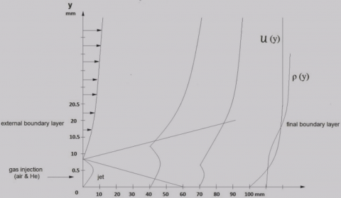
For the final regime the external flow supersedes the wall jet and gets near of the turbulent boundary layer together with the normal density gradient. Both flows approach one another as the fluid moves forward. The air or helium meets the external fluid at some points forming a completely developed turbulent flow. At x=100mm from the injection slot: boundary layer thickness $\delta=20.5 m m, R e_{\delta}=6000$ the flow situation is sketched in Figure 1.
Turbulent wall jet flows with strong density differences are ubiquitous in nature as well as in industry, such as in the diffusion flames. They are also apparent over strongly heated walls mainly when a space ship re-enters the atmosphere, and in aeronautics: in compressible subsonic, transonic and supersonic, such as high speed aircraft flight.
Figure 1. Flow situation
Major industrial applications are in confined flow, such as in internal combustion engines; where the compressibility and mixture between different mass species can be used together in order to enhance mixing. Consequently, they improve the engine efficiency and reduce the generation of pollutants [11, 12]. There are other applications: the film cooling at the level of the combustion chamber and the stage of the gas-turbine. In the case of combustion chamber as well as stage of the gas-turbine the target is to insert a cool fluid through the wall so as to preserve the surface from exposure to a hot external fluid, where various parameters should be considered: The gradient of velocity, temperature, and density [13]. The manufacture of metal or glass plates mainly during the annealing phase is an example of the use of wall jet which is the result of jet impingement on a surface. The wall jet is responsible for half the consumed energy in transporting fluids through pipes.
Among other applications is the diminution of the wall shear stress,$\tau_{\omega}$, through a decrease in density on the boundary layer due to an electrostatic phenomenon: induced positive surface charge repulsion as a result of the ionization of the air at hypersonic speeds [14], or by using the two scale character in the flow, since there is an interaction between the external large eddies and the inner small ones. The slightest modification of the large eddies leads to alteration of the small eddies which helps to diminish the wall shear stress, and ultimately to reduce fuel consumption in an aircraft flying at cruise. [15, 16].
The physical properties of fluids vary according to changes of density variations. The transfer coefficients especially at a solid boundary layer cause such changes, even at low speed flows.
Adopting improved hot-wire and, laser Doppler anemometry, many studies in the decade of 1990s - 2000s [7, 17-21], ended with the following conclusions: A transition region of about 20-30e long succeeded by a developed flow. Two main factors influence the flow; the velocity ratio r and less severely the density ratio S. Low values of S increase all of three elements: first, turbulence, especially in the transition region, which is consequently shorter in this case; second, velocity near the wall. This may be due to the enhancement of large-scale coherent structures as seen by visualization and confirmed by an important correlation between density and velocity fluctuation, and third the friction velocity $u_{\tau}$ if obtained from the log law.
The fundamental motivation of this research resides very particularly in the fact that the coupling equations of thermodynamic conservation and of the mechanics (mass, momentum etc.) become stronger considering the density variation, especially that the natural phenomena and industrial applications are of a variable density. Our aim, hence, is to highlight the influence of the variable density on turbulent wall jets and how to use this variation in order to enhance the physical parameters, such as mixture, for a better combustion, or the reduction of the wall shear for example.
Using RANS (Reynolds stress model), the present numerical study has as aim to mimic the first part of the experimental work of Soudani et Al concerning the dynamics and mixing of a wall jet at Reynolds number similar to those in the experiments. It serves as an introduction to the second part of experience which will be held in the future using LES method. Therefore, after estimating the large and Kolmogorov scales using RANS it will be possible to obtain LES mesh to access the instant variable in the experience. The whole study is by that time recalculated with LES simulation, where the higher order statistics as skewness and flatness factors $\frac{\overline{u^{'3}}}{\left(\sqrt{\overline{u^{'2}}}\right)^{3}}, \frac{\overline{\rho^{'3}}}{\left(\sqrt{\overline{\rho^{\prime 2}}}\right)^{3}}, \frac{\overline{u^{'4}}}{\left(\sqrt{\overline{u^{'2}}}\right)^{4}}, \frac{\overline{\rho^{\prime4}}}{\left(\sqrt{\overline{\rho^{\prime 2}}}\right)^{4}}$ and correlation coefficient $R_{-\overline{\rho v}}=\frac{-\overline{\rho^{\prime} v^{\prime}}}{\sqrt{\overline{\rho^{\prime} \rho^{\prime}}} \sqrt{\overline{v^{\prime} v^{\prime}}}}$ will be considered.
New correlations as $\overline{\rho f^{\prime}}$ represent a challenge for this numerical study. For this reason, we used the notion mass-weighted introduced by Favre in a series of publications [22-27]. This average permits formally to find an equation system similar to those obtained in a flow with constant density, and thus the term $\overline{\rho f^{\prime}}$ implicitly contributes to the mean momentum balance equation.
All variables in mean equations are computed with the Favre average (mass-weighted) except for the pressure and the density. The latter are always computed using Reynolds’ average. This quantity is defined as
$\tilde{F}=\frac{\overline{\rho F}}{\bar{\rho}}$ (1)
with
$F=\tilde{F}+f^{\prime \prime}$ with $\overline{f^{\prime \prime}} \neq 0 \overline{\rho f}^{\prime \prime}=0$ (Favre) $F=\bar{F}+f^{\prime}$ with $\overline{f^{\prime}}=0 \overline{\rho f^{\prime}} \neq 0$ (Reynolds)
2.1 Average equation of the continuity
We can write now: $\rho U_{j}=\rho \widetilde{U}_{j}+\rho u_{j}^{\prime \prime}$.
Taking the average, we obtained: $\overline{\rho U_{j}}=\bar{\rho} \widetilde{U}_{j}$ since $\overline{\rho u_{j}^{\prime \prime}}=0$
$\frac{\partial\left(\bar{\rho} \widetilde{U_{J}}\right)}{\partial x_{j}}=0$ (2)
2.2 Average equation of the momentum conservation
In the same way we obtain:
$\frac{\partial \bar{\rho} \widetilde{U}_{i} \widetilde{U}_{j}}{\partial x_{j}}=\bar{\rho} g_{i}-\frac{\partial \bar{P}}{\partial x_{i}}+\frac{\partial}{\partial x_{j}}\left[\bar{\mu}\left(\frac{\partial \widetilde{U}_{i}}{\partial x_{j}}\right)-\left(\bar{\rho} \widetilde{u_{l}^{\prime \prime} u_{J}^{\prime \prime}}\right)\right]$ (3)
2.3 Average equation of the mixture fraction conservation
$\frac{\partial \bar{\rho} \tilde{c} \widetilde{U}_{j}}{\partial x_{j}}=\frac{\partial}{\partial x_{j}}\left[D \frac{\partial \tilde{C}}{\partial x_{j}}-\left(\bar{\rho} \widetilde{c^{\prime \prime} u_{J}^{\prime \prime}}\right)\right]$ (4)
Out of the equation of state we calculate the mean density from the mean mass fraction. With constant pressure, this leads to
$\frac{1}{\rho}=\frac{C}{\rho_{1}}+\frac{1-C}{\rho_{2}}, \rho=a \rho C+b, a=\frac{\rho_{1}-\rho_{2}}{\rho_{1}}, b=\rho_{2}$ (5)
The mixture viscosity is calculated by ANSYS based on the kinetic theory as:
$\mu=\sum i \frac{X_{i} \mu_{i}}{\sum_{j} X_{j} \emptyset_{i j}}$ (6)
where, $\varnothing_{i j}=\frac{\left[1+\left(\frac{\mu_{i}}{\mu_{j}}\right)^{1 / 2}\left(\frac{M_{w, j}}{M_{w, i}}\right)^{1 / 4}\right]^{2}}{\left[8\left(1+\frac{M_{w, i}}{M_{w, j}}\right)\right]^{1 / 2}}$.
And $X_{i}$ represent the mole fraction of species i.
The turbulent stresses and the turbulent mass fraction fluxes seen in the precedent equations are novel correlations which necessitate a modelling.
2.4 Species transport equations
By analogy, the term which represents the turbulent mass fraction flux is estimated by using gradient diffusion expression:
$\frac{\partial \bar{\rho} \tilde{C} \tilde{U}_{j}}{\partial x_{j}}=\frac{\partial}{\partial x_{j}}\left[\left(D+\frac{\vartheta_{t}}{\sigma_{t}}\right) \frac{\partial \tilde{C}}{\partial x_{j}}\right]$ (7)
2.5 Second moment closure
The second order modelling advantage is that each of Reynolds stresses is calculated on the basis of their proper transport equations. It is thus, the appropriate model to study the anisotropic turbulence and best describe the influence of variable density [28-30].
The exact transport equation for the Reynolds stresses is of the form:
$\frac{\partial\left(\overline{\rho u^{\prime \prime}{ }_{\imath} u_{j}^{\prime \prime}}\right) U_{k}}{\partial x_{k}}=P_{i j}+G_{i j}+\emptyset_{i j}+d_{i j}-\rho \epsilon_{i j}$ (8)
where
$P_{i j}=-\bar{\rho}\left(\widehat{u_{\imath}^{\prime} u^{\prime \prime}}_{k} \frac{\partial \widetilde{U}_{j}}{\partial x_{k}}+\widetilde{u^{\prime \prime} u^{\prime \prime}}_{k} \frac{\partial \widetilde{U}_{i}}{\partial x_{k}}\right)$
$G_{i j}=-\frac{\mu_{t}}{\rho P r_{t}}\left(g_{i} \frac{\partial \bar{\rho}}{\partial x_{j}}+g_{j} \frac{\partial \bar{\rho}}{\partial x_{i}}\right)$
The turbulence kinetic energy tends to increase in unstable stratification $G_{i j}>0$. For stable stratification, buoyancy tends to suppress the turbulence $G_{i j}<0$.
2.5.1 Modelling turbulent diffusive transport
$d_{i j}$ Can be modelled by the generalized gradient-diffusion model of Daly and Harlow [31]:
$D_{i j}=C_{s} \frac{\partial}{\partial x_{k}}\left(\bar{\rho} \frac{k \partial \widetilde{u_{k}^{\prime \prime} u_{l}}^{\prime \prime}}{\epsilon} \frac{\partial \partial \widetilde{u_{i}^{\prime \prime} u_{j}^{\prime \prime}}}{\partial x_{l}}\right)$
Numerical divergence results from this equation, however. That’s why ANSYS Fluent uses a scalar turbulent diffusivity as follows:
$D_{i j}=\frac{\partial}{\partial x_{k}}\left(\frac{\mu_{t}}{\sigma_{k}} \frac{\partial \widetilde{u_{i}^{\prime \prime} u_{j}^{\prime \prime}}}{\partial x_{l}}\right)$
The turbulent viscosity, $\mu_{t}$ , is computed using $\mu_{t}=\rho C_{\mu} \frac{k^{2}}{\epsilon}$
$C_{\mu}$ Empirical constant $C_{\mu}=0.09$
$\sigma_{k}$ Turbulent Prandtl number $\sigma_{k}=0.82$.
2.5.2 Modelling $\emptyset_{i j}$ the redistribution term
$\emptyset_{i j}$ Which is a redistribution term doesn’t affect the value of k. Three main divisions make up the pressure strain correlation modelling: $\emptyset_{i j}=\emptyset_{i j 1}+\emptyset_{i j 2}+\emptyset_{i j w}$.
$\emptyset_{i j 1}$ which as a slow term, depends only on velocity fluctuation and expresses a return to isotropy. It is modelled as follows:
$\emptyset_{i j 1}=-C_{1} \frac{\bar{\rho} \epsilon}{k}\left(\widetilde{u_{l}^{\prime \prime} u_{j}^{\prime \prime}}-\frac{2}{3} \delta_{i j}\right)$, where $C 1=1.8$.
$\emptyset_{i j 2}$ Which as a rapid term, depends on velocity fluctuation and average velocity gradient and also expresses a return to isotropy: $\emptyset_{i j 2}=-C_{2}\left[\left(P_{i j}-C_{i j}\right)-\frac{2}{3} \delta_{i j}(P-C)\right]$, where $C_{2}=0.6, P=\frac{1}{2} P_{k k}$ and $C=\frac{1}{2} C_{k k}$ .
The reflection term of the wall, $\emptyset_{i j w}$ , tends to damp the stress normal to the wall.
$\emptyset_{i j w}=\rho C_{1}^{\prime} \frac{\epsilon}{k}\left(\widetilde{u_{k}^{\prime \prime} u_{m}^{\prime \prime}} n_{k} n_{m} \delta_{i j}-\frac{3}{2} \widetilde{u_{i}^{\prime \prime} u_{k}^{\prime \prime}} n_{j} n_{k}-\frac{3}{2} \widetilde{u_{j}^{\prime \prime} u_{k}^{\prime \prime}} n_{i} n_{k}\right)\left(\frac{C_{l} l}{y}\right)+C_{2}^{\prime}\left(\emptyset_{k m, 2} n_{k} n_{m} \delta_{i j}-\frac{3}{2} \emptyset_{i k, 2} n_{j} n_{k}-\frac{3}{2} \emptyset_{j k, 2} n_{i} n_{k}\right)\left(\frac{C_{l} l}{y}\right)$
In this equation $n_{l}$ represents the unit vector normal to the wall, and y is the distance from the wall, while l is the turbulence length scale.
$C_{1}^{\prime}=0.5, C_{2}^{\prime}=0.3, C_{l}=\frac{c_{\mu}^{2 / 4}}{\mathrm{\kappa}}, C_{\mu}=0.09, \mathrm{\kappa}=0.4187$ (the von Karman constant).
2.5.3 Modelling of the dissipation rate
The equation of the dissipation rate of turbulent kinetic energy $\epsilon$ is modelled in the same manner as that of k- $\epsilon$ model.
$\frac{\partial \rho U_{k} \epsilon}{\partial x_{k}}=\frac{\rho \epsilon^{2}}{k}\left(c_{\epsilon 1} \frac{P_{k}}{\rho \varepsilon}-c_{\epsilon 2}\right)+\frac{\partial}{\partial x_{k}}\left(\left(\mu+\frac{\mu_{t}}{\sigma_{\epsilon}}\right) \frac{\partial \epsilon}{\partial x_{k}}\right)$ (9)
where, $c_{\epsilon 1}=1.44, c_{\epsilon 2}=1.92$ and $\sigma_{\epsilon}=1.44$
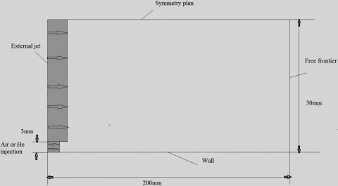
3.1 Boundary conditions
Frontiers types surrounding the domain are presented on Figure 2.
3.1.1 The entrance
In the external flow, we have $\rho_{\infty}=1 \mathrm{~kg} / \mathrm{m}^{3}, U_{\infty}=$ $5.8 \mathrm{~m} / \mathrm{s}$ and $\tilde{C}_{\infty}=0$. Concerning turbulence parameters we have chosen the intensity and length scale method for initial condition, and used the boundary layer thickness, $\delta_{99}$, to estimate the turbulent length scale, $l$, from $l=0.4 \delta_{99}$
In the internal flow, we have an injection of pure air $\left(\rho_{i n j}=\right.$ $1.2 \mathrm{~kg} / \mathrm{m}^{3}$, or pure helium $\rho_{i n j}=0.16 \mathrm{~kg} / \mathrm{m}^{3}$ where $\tilde{C}_{i n j}=$ 1 through a slot of height $3 \mathrm{~mm}$, with bulk velocity $U_{i n j}=$ $2 \mathrm{~m} / \mathrm{s}$.
The dissipation rate $\epsilon=\frac{k^{1.5}}{l}$, where $l$ represents the large eddies scale on entrance which is expressed on fluent in function of mixing length $l_{m}$ as $l=c_{\mu}^{-3 / 4} l_{m}$, where, $l_{m}$ is determined from hydraulic diameter $D_{H}$ prescribed on entrance $l_{m}=0.07 D_{H}$ where $D_{H}=2 e$.
The Reynolds shear stresses: $\overline{u_{\imath} u_{J}}=\frac{2}{3} k \delta_{i j}$; the normal stresses are equal and the tangential are null, which means an isotropic turbulence.
3.1.2 Wall
No slip condition is imposed at wall in conjunction with specific wall treatment. The Reynolds shear stresses are calculated explicitly by the code as follows: $\frac{\widetilde{u_{t}^{\prime \prime 2}}}{k_{p}}=1.098 ; \frac{\widetilde{u_{n}^{\prime \prime 2}}}{k_{p}}=0.247 ; \frac{\widetilde{u_{Y}^{\prime \prime 2}}}{\mathrm{k}_{\mathrm{p}}}=0.655 ;-\frac{u_{\tau}{ }^{\pi} u_{n}^{\prime \prime}}{k_{p}}=0.255$. Where, $\tau$ is the tangential direction at the wall, n is the normal direction and $\gamma$ is the transversal direction.
The near wall treatment choice submits to some remarks and considerations:
The slot size of 3mm compels severe demands on mesh resolution near the wall. Still, it is impossible to ensure that the first point in the mesh lies in the logarithmic zone imposed by standard wall function. The latter, which has a universal character, is restricted to large y+, where the pressure gradient is impact less. Nevertheless, in our flow there exists the velocity gradient between injection jet through the slot and external jet which provokes pressure gradient, and we depart from the ideal condition and get away from universality.
On the light of these remarks, we have chosen to enhance wall function treatment which allows a more flexible meshing, permitting the grid to begin at low y+.
3.1.3 Free frontiers
Free frontiers are free internment frontiers of the fluid where the pressure is constant and equals atmospheric pressure which is known. It is the velocity, however, which is calculated from the continuity equation implicated locally at cells near frontiers.
3.1.4 Symmetry plan
The gradient for any dependent variable $\emptyset$ normal to the symmetry plan, and The Reynolds shear stress vanish $\frac{\partial \emptyset}{\partial y}=0, \widetilde{u^{\prime \prime} v^{\prime \prime}}=0$.
The normal velocity component to the symmetry plan is imposed zero V=0.
Figure 2. Domain frontiers
3.2 Mesh
To generate a mesh of high quality, the refined mesh was affected at the level of two zones, the first is the mixture layer between the external jet and the injection jet through a slot at a level of separation line at the nozzle exit, and the second is near the wall to capture steep gradients for different variables. A mesh free solution can be obtained when a grid consists of (70 Х 200). The first line is 0.07mm far from the wall (Figure 3).
Figure 3. Mesh
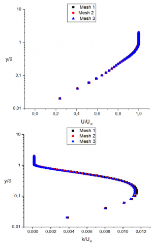
The choice of this mesh was only done after the study of the grid effect on the result by comparing between 03 meshes with different node numbers 10400, 11600, 14000, which correspond to 6, 12, 24 divided at exit jet level.
Figure 4 shows that turbulent energy is a little more sensitive to velocity as regards the different meshes. The mesh 2, 3 give a similar profile that’s why we adopted mesh 03.
Figure 4. Mesh effect on the results
3.3 Preliminary calculations
3.3.1 Y plus estimation
The Figure 5 shows the distribution of y+ all the way through the wall, the values are between 0.2 and 2. These values are too small to intrude through the inner boundary layer of wall jet.
Figure 5. Y+ distributions along the wall
3.3.2 Scales
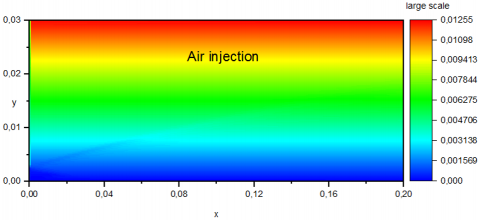
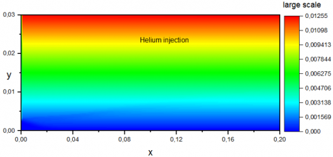
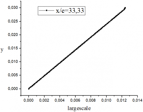
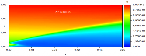
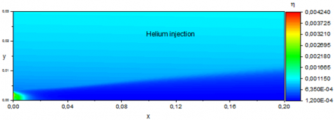
Figure 6. Large and Kolmogorov scales
The contours presented in Figure 6 show the large and Kolmogorov scales estimated respectively by $l=\frac{k^{\frac{3}{2}}}{\epsilon}$ and $\eta=\left(\frac{v^{3}}{\epsilon}\right)^{\frac{1}{4}}$. The results show that near the wall the size of large scale is 1mm and the Kolmogorov scale is 0.1mm. Far from the wall the large scale increases along of the y direction to reach the value less than 12.5mm, but the Kolmogorov scale has 1mm for both injections. These results confirm that the large eddies vary in a linear way $(l=\mathrm{Ky})$ with $\mathrm{K}$the Karman constant. We also notice that moving toward the wall the large eddies transform into smaller eddies and get nearer to the Kolmogorov eddies [32].
4.1 Velocity
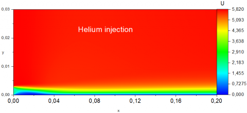
The velocity profiles are but slightly affected by the gas injected, however the helium injection gives a way to a slightly superior average velocity near the wall see Figure 7.
Figure 7. Plot of mean velocity in different stations
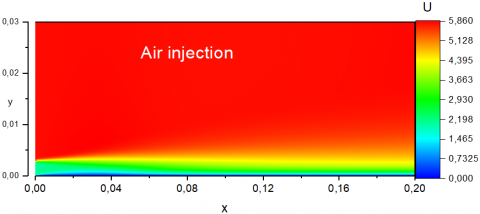
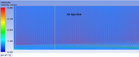
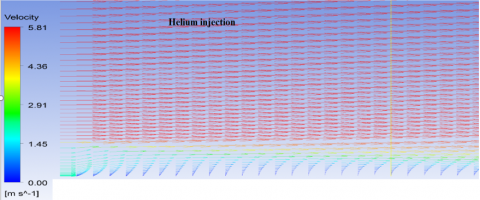
In the case of helium injection, the light fluid situated on the edge of the internal jet is strongly accelerated by the entrainment of the heavy external fluid in the mixture layer. Correlatively, by conservation of momentum, the flow is decelerated in the vicinity of the wall. The entrainment creates a depression of internal fluid whose strength is measured with the dynamic pressure of the internal jet $\frac{1}{2} \rho_{i} U^{2}$. When the depression is sufficiently important, an attachment zone is installed near the wall. However, the heavy external fluid situated on the edge of the mixture layer is slightly decelerated compared to the case of heavy air injection, which explains why the average velocity becomes higher by injecting helium. Check contour and vector velocity in Figures 8, 9.
Figure 8. Contour velocity
Figure 9. Velocity vector
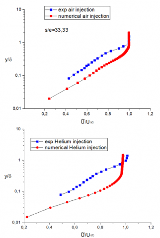
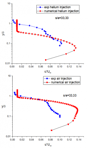
4.1.1 Numerical versus experimental velocity
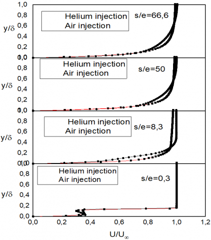
The comparison of the velocity to experimental results at s/e=33.33 station shows that the numerical velocity rises steeply from the wall to $\frac{y}{\delta}<0.15$ (Figure 10).
The deviation between the experimental data and the numerical data is due essentially to the initial condition, where the turbulent external jet in the experiment is a developed turbulent boundary layer with $U_{\infty}$ 5.8m/s and δ= 20mm. However, in the numerical simulation we opted for a uniform profile with $U_{\infty}$ velocity, which resulted in very important velocity gradient near the wall in comparison with the experiment.
Figure 10. Comparison between numerical and experimental results of the velocity
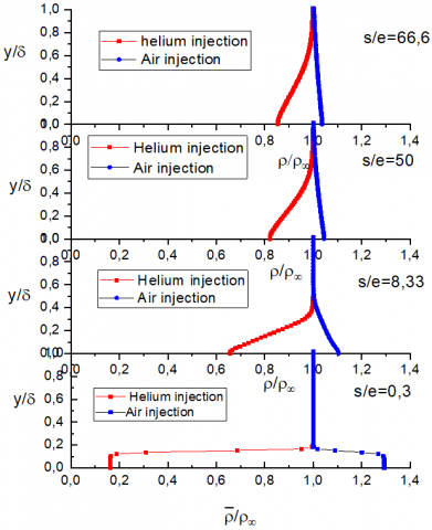
4.2 Density
Figure 11. Plot of mean density in different stations
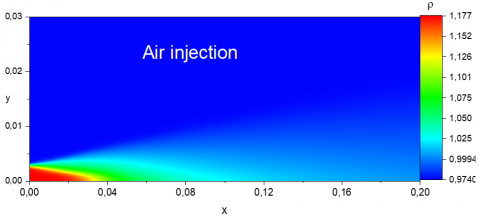
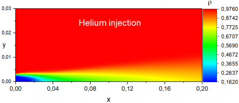
The density profile evolution presented in Figure 11 shows the very quick dilution and strong gradient density in the initial zone of the flow. The same results are witnessed in contour density in Figure 12. This gradient reaches asymptotic behaviour for which the ratio of density develops slowly with x, and tends to the value of about 0.8 in the helium injection case.
Figure 12. Density contour
4.2.1 Numerical versus experimental density
Figure 13 shows that the numerical profile is globally in good accordance with the experimental results. However, the mixing and dilution is better in the helium injection.
Figure 13. Comparison between numerical and experimental results of density
4.3 Turbulence
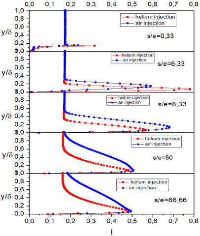
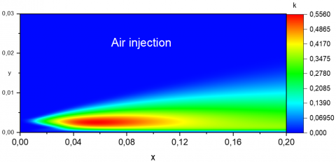
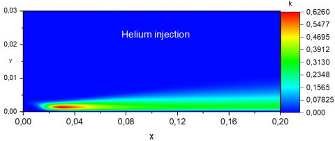
Near the wall region, the turbulent intensity $I=\sqrt{\frac{2}{3} k}$ is reinforced by helium injection, and it develops more rapidly than the air injection for $y /_{\delta}<0.2$ see Figure 14. This is confirmed respectively by turbulence kinetic energy contour Figure 15, Figure 17 and Figure 18. The previous results are due to the instable situation where the turbulence intensity and the entrainment increase because of the buoyancy effect.
Figure 14. Plot of turbulent intensity in different stations
Figure 15. Turbulent energy contour
4.3.1 Numerical versus experimental turbulence intensity
Longitudinal velocity fluctuation intensity $\frac{u \prime}{U_{\infty}} \cong 10 \%$ (Shlichting) [33], is in accordance with experimental results. The numerical values reach 13% for air and 14% for helium at $y /_{\delta} \cong 0.2$ far from the wall, in the region where the average flow is perfectly uniform $\frac{U^{\prime}}{U_{\infty}} \cong 1$. The velocity fluctuation should be very small $\frac{u \prime}{U_{\infty}} \cong 0.5$, the numerical value gives a level of fluctuation approximately 1%. So, we notice a small over estimation of turbulence (Figure 16).
Figure 16. Comparison between numerical and experimental results of stream wise velocity fluctuation
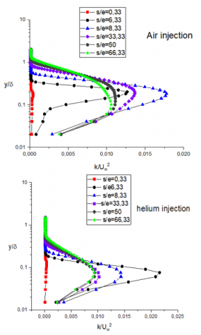
Figure 17. Semi-logarithmic plot of turbulent kinetic energy in different stations
4.3.2 Turbulent kinetic energy in different stations
Figure 17 shows the superposition of the turbulent energy in different stations. While the wall jet moves downstream, an intensification of turbulence is noticed in a developing region.
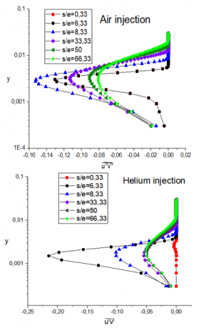
4.3.3 Tangential stresses in different stations
Figure 18 shows that $\overline{u^{\prime \prime} v^{\prime \prime}}$ is negative because in the presence of $\frac{\partial U}{\partial y}>0$ near the wall then a positive $v^{\prime \prime}$ correlates with a negative $u^{\prime \prime}$ and this is a phenomenological understanding of why $\overline{u^{\prime \prime} v^{\prime \prime}}$ tends to be negative in parallel shear flow.
Figure 18. Semi-logarithmic plots of tangential stresses in different stations
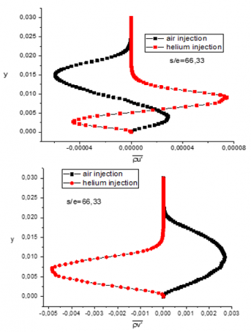
4.3.4 Correlations $\overline{\rho v^{\prime}}, \overline{\rho u^{\prime}}$
This correlation is an important variable to understand the effect of density differences on the behaviour of turbulent structure in boundary layer. In this study, we use a generalized gradient diffusion expression of the form: $\overline{\rho u_{l}}=-D_{t} \frac{\partial \bar{\rho}}{\partial x_{i}}$.
In the case of air injection, the $\overline{\rho v^{\prime}}$ is positive because we have $\frac{\partial U}{\partial y}>0$ and $\frac{\partial \rho}{\partial y}<0$; the internal motion ($v^{\prime}<0$) with lighter fluid portions ($\rho<0$). Doing the average, we obtain a positive correlation between density and velocity fluctuation following y direction, in external motion. However, when $v^{\prime}>0$ with heavier fluid portions $\rho>0$ we always obtain a positive correlation. The same reasoning goes for the other cases see Figure 19.
4.4 Along of the wall
Along the developing boundary layer, we notice that the jet develops very fast in case of helium injection rather than in air injection, which provokes an important downfall of skin friction near the wall see Figure 20.
Figure 19. Correlations between density and velocity fluctuation
Figure 20. Shear wall, velocity shear and average density profiles respectively
Figure 20 also shows that the transition region stretches approximately up to a length of about 30 e followed by a region of developed flow.
Compared to the experimental results, the numerical ones are very encouraging. They confirm the results obtained in the experiment:
The density and velocity gradients contribute in the production of turbulent energy. The results show that the downstream region (until 30e) is characterized by a sluggish restoration to equilibrium towards a standard boundary layer regime. In this region, the local density gradient does not participate in a significant way to the turbulent energy. However, the turbulence structure modification is the result of the memory effect of initial perturbations.
This study also made it possible to estimate eddies large and Kolmogorov scales expressed respectively through $l=\frac{k^{\frac{3}{2}}}{\epsilon}$ and $\eta=\left(\frac{v^{3}}{\epsilon}\right)^{\frac{1}{4}}$, so as to study the instantaneous, three-dimensional flows. The mesh will be extruded to third direction between two periodic frontiers with the distance of 2.5 times the size of large eddies scale and the spatial discretization equal 12 times the size of Kolmogorov scale [34, 35] to access to the instantaneous values in the experience study as skewness and flatness factors $\frac{\overline{u^{'3}}}{\left(\sqrt{\overline{u^{2\prime}}}\right)^{3}}, \frac{\overline{\rho^{\prime3}}}{\left(\sqrt{\overline{\rho^{\prime2}}}\right)^{3}}, \frac{\overline{u^{'4}}}{\left(\sqrt{\overline{u^{\prime2}}}\right)^{4}}, \frac{\overline{\rho^{'4}}}{\left(\sqrt{\overline{\rho^{\prime 2}}}\right)^{4}}$.
The computations were carried out at LPEA Laboratory University of Batna 1, to which I am much grateful for providing the original version of the Ansys software licensing. The purposeful discussions with Pr Zoubir Nemouchi, Professor at the Mechanics Institute in Constantine University, were of paramount importance to this study.
|
$\tilde{C}$ |
Density-weighted mass fraction of helium jet |
|
C1, C1, C2, Cϵ1, Cϵ2 |
Second moment closure constants |
|
D e $\bar{F}$ $f^{\prime}$ |
Mass diffusivity, m2s-1 Slot height, m Average scalar function Scalar fluctuation |
|
g |
Gravitational acceleration, m.s-2 |
|
Gk |
Term of production due to buoyancy forces, kg.m-1.s-3 |
|
k l lm |
Kinetic energy of turbulence, m2s-2 Large eddies scale, m Mixture length, m |
|
Pk |
Term of production due the mean gradient, kg. m-1s-3 |
|
Reτ |
Reynolds-number based on momentum thickness |
|
uτ $\widetilde{U}$ |
Friction velocity, m.s-1 Density-weighted mean flow velocity component, m |
|
Greek symbols |
|
|
ϵ |
Turbulent dissipation rate, m2s-3 |
|
$\phi_{i j}$ |
Pressure-strain term in turbulence model |
|
σk ,σϵ |
Prandtl number for turbulence energy and dissipation rate |
|
η δ99 |
Kolmogorov scale, m Boundary-layer thickness of 99%, m |
|
µ, µt |
Dynamic molecular and turbulent viscosity, kg. m-1.s-1 |
|
ν ρ $\overline{\rho f^{\prime}}$ к τ |
Kinematic viscosity, m2.s-1 Density, kg.m-3 Density scalar fluctuation correlation Von Karman constant Wall shear, Pa |
|
Subscripts |
|
|
τ |
Tangential direction at the wall |
|
γ |
Transversal direction |
[1] Dejoan, A., Leschziner, M.A. (2005). Large eddy simulation of a plane turbulent wall jet. Physics of Fluids, 17(2): 025102. https://doi.org/10.1063/1.1833413
[2] Dejoan, A., Leschziner, M.A. (2004). LES study of the statistical characteristics of the plane turbulent wall jet. Physics of Fluids, 17(2): 663-666. https://doi.org/10.1063/1.1833413
[3] Djoan, A., Leschziner, M.A. (2005). Assessment of turbulence models for predicting the interaction region in a wall jet by reference to LES solution and budgets. ETMM6, Sardinia, Italy.
[4] Ahlman, D., Brethouwer, G., Johansson, A.V. (2007). Direct numerical simulation of a plane turbulent wall-jet including scalar mixing. Physics of Fluids, 19(6): 065102. https://doi.org/10.1063/1.2732460
[5] Launder, B.E., Rodi, W. (1983). The turbulent wall jet measurements and modeling. Annual Review of Fluid Mechanics, 15(1): 429-459. https://doi.org/10.1146/annurev.fl.15.010183.002241
[6] Dejoan, A., Leschziner, M.A. (2006). Separating the effects of wall blocking and near-wall shear in the interaction between the wall and the free shear layer in a wall jet. Physics of Fluids, 18(6): 065110. https://doi.org/10.1063/1.2212991
[7] Harion, J. (2003). Density and velocity measurements in turbulent he-air boundary layers. Sciences & Technologie, (19): 70-75.
[8] Livescu, D. (2020). Turbulence with large thermal and compositional density variations. Annual Review of Fluid Mechanics, 52: 309-341. https://doi.org/10.1146/annurev-fluid-010719-060114
[9] Xu, D., Chen, J. (2016). Subgrid-scale dynamics and model test in a turbulent stratified jet with coexistence of stable and unstable stratification. Journal of Turbulence, 17(5): 443-470. https://doi.org/10.1080/14685248.2015.1129407
[10] Chassing, P. (2001). The modelling of variable density turbulence flow. A review of first-order closure schemes. Flow, Turbulence and Combustion, 66: 293-332. https://doi.org/10.1023/A:1013533322651
[11] Bouras, F., Si-Ameur, M., Soudani, A. (2013). Large eddy simulation for lean premixed combustion. The Canadian Journal of Chemical Engineering, 91(2): 231-237. https://doi.org/10.1002/cjce.21642
[12] Bouras, F., Soudani, A., Si-Ameur, M. (2012). Numerical study of the turbulent flow inside an ORACLES configuration. Journal of Applied Mechanics, 79(5): 51014. https://doi.org/10.1115/1.4006455
[13] Sarkar, S., Bose, T.K. (1995). Comparison of different turbulence models for prediction of slot-film cooling: flow and temperature field. Numerical Heat Transfer, Part B Fundamentals, 28(2): 217-238. https://doi.org/10.1080/10407799508928831
[14] Selvakumar, A., Palanisamy, S. (2020). Analysis of the effects of positive ions and boundary layer temperature at various hypersonic speeds on boundary layer density. Emerging Investigators. https://www.emerginginvestigators.org/articles/analysis-of-the-effects-of-positive-ions-and-boundary-layer-temperature-at-various-hypersonic-speeds-on-boundary-layer-density.
[15] Viswanath, P.R. (2002). Aircraft viscous drag reduction using riblets. Progress in Aerospace Sciences, 38(6-7): 571-600. https://doi.org/10.1016/S0376-0421(02)00048-9
[16] Airline fuel cost and consumption. (2016). (U.S. Carriers-Scheduled) Retrieved from United State Department of Transportation. www.transtats.bts.gov/fuel.asp.
[17] Riva, R., Binder, G., Favre-Marinet, M., Harion, J.L. (1994). Development of turbulent boundary layer with large density gradients. Experimental Thermal and Fluid Science, 9(2): 165-173. https://doi.org/10.1016/0894-1777(94)90109-0
[18] Harion, J.L., Favre-Marinet, M., Camano, B. (1996). An improved method for measuring velocity and concentration by thermo-anemometry in turbulent helium-air mixtures. Experiments in Fluids, 22(2): 174-182. https://doi.org/10.1007/s003480050035
[19] Harion J.L., Soudani A., Royer J.C., Tardu S., Binder G. (1996). Application of neural networks to simultaneous measurements in turbulent flows. Comptes Rendus de l’Academie des Sciences, série II, 318(11): 1445-1452. https://scholar.google.fr/citations?view_op=view_citation&hl=fr&user=RHP75I4AAAAJ&cstart=20&pagesize=80&citation_for_view=RHP75I4AAAAJ:hMod-77fHWUC.
[20] Soudani, A., Bougoul, S., JL Harion, J.L. (2003). Density and velocity measurements in turbulent He-Air boundary layers. Sciences & Technologie. A, Sciences Exactes, 19: 70-75. http://revue.umc.edu.dz/index.php/a/article/view/1835.
[21] Soudani, A., Marinet, M.F., Tardu, S., Harion, J.L. (1996). Fine structure of turbulence in a boundary layer with strong density differences. Advances in Turbulence VI, pp. 295-298.
[22] Favre, A. (1958). Equations statistiques des gaz turbulent. CR. Acad. Sci Paris, 246: 2573-3216.
[23] Favre, A. (1965). Equations des gaz turbulents compressibles’ I Forme générales. J. Méc., 4: 361-390.
[24] Favre, A. (1965). Equations des gaz turbulents compressibles’. II Méthode des vitesses moyennes; Méthode des vitesses macroscopiques pondérées par la masse volumique. J. Méc., 4: 390-421.
[25] Favre, A. (1971). Equations statistique aux fluctuations d’entropie, de concentration, de rotationnel dans les écoulements compressibles. C.R. Acad. Sci. Paris, 273: 1289-1294.
[26] Favre, A. (1975). Equations statistique des fluides turbulents compressibles. Fifth Cong. Can. De Méc. Appl., New Brunswick Univ., pp. G3-G34.
[27] Favre, A. (1992). Formulation of the statistical equations of turbulent flows with variable density. Studies in Turbulence, 324-341. https://doi.org/10.1007/978-1-4612-2792-2_23
[28] Chassaing, P., Herard, J.M. (1987). Second order modelling of variable density turbulent mixing. In 6th Symposium on Turbulent Shear Flows.
[29] Chassaing, P., Ghibat, M. (1988). Second order modelling of a variable density mixing layer’. Euromech. Coll. 37, Marseille, France.
[30] Chassaing, P., Harran, G., Joly, L. (1994). Density fluctuations correlations in free turbulent binary mixing. Journal of Fluid Mechanics, 279: 239-278 https://doi.org/10.1017/S0022112094003903
[31] Daly, B.J., Harlow, F.H. (1970). Transport equations in turbulence. Physics of Fluids, 13: 2634-2649.
[32] Shih, T.H., Lumley, J.L. (1992). Kolmogorov behavior of near-wall turbulence and its application in turbulence modeling (Vol. 105663). National Aeronautics and Space Administration.
[33] Schlichting, H., Kestin, J. (1961). Boundary Layer Theory (Vol. 121). New York: McGraw-Hill.
[34] Verteeg, H., Malalasekra, W. (2007). An Introduction to Computational Fluid Dynamics: The Finite Volume Method’ Second edition. Pearson Education Limited. Edinburgh Gate, Harlow. Essx CM20 2JE. England.
[35] Hadžiabdić, M., Hanjalić, K. (2008). Vortical structures and heat transfer in a round impinging jet. Journal of Fluid Mechanics, 596: 221-260. https://doi.org/10.1017/S002211200700955X