Abduvali Khaldjigitov | Umidjon Djumayozov* | Dilnoza Sagdullaeva
© 2021 IIETA. This article is published by IIETA and is licensed under the CC BY 4.0 license (http://creativecommons.org/licenses/by/4.0/).
OPEN ACCESS
The article considers a numerical method for solving a two-dimensional coupled dynamic thermoplastic boundary value problem based on deformation theory of plasticity. Discrete equations are compiled by the finite-difference method in the form of explicit and implicit schemes. The solution of the explicit schemes is reduced to the recurrence relations regarding the components of displacement and temperature. Implicit schemes are efficiently solved using the elimination method for systems with a three diagonal matrix along the appropriate directions. In this case, the diagonal predominance of the transition matrices ensures the convergence of implicit difference schemes. The problem of a thermoplastic rectangle clamped from all sides under the action of an internal thermal field is solved numerically. The stress-strain state of a thermoplastic rectangle and the distribution of displacement and temperature over various sections and points in time have been investigated.
thermoplasticity, displacement, temperature, stress, differential equation, explicit scheme, convergence
At the present stage of development of science and technology, the study of the stress-strain state of structures and their elements, in order to determine their strength and reliability margins, taking into account thermomechanical elastoplastic deformations, is an urgent task of scientific and technical applications.
Mathematical models describing the process of heat propagation were first considered in the works [1-4], in which it was assumed that total deformation consists of elastic deformation and thermal expansion
The problems of the theory of thermoplasticity were first considered in more detail in the works [5-7], and it was assumed that the total deformation consists of elastic, plastic and thermal deformations. Further, these studies were continued in the works [8-16].
The plasticity theories for isotropic and anisotropic materials and an effective numerical method of plasticity were considered in [17-19]. The finite-difference methods for different coupled and uncoupled boundary value problems, within the framework of thermodynamic laws, were considered in the works [20-26].
When solving problems of thermoelasticity and thermoplasticity, usually, the temperature distributions were determined in advance based on the solution of the heat flow equation, and when solving boundary value problems of thermoelasticity and thermoplasticity, the temperature terms considered in combination with volume forces.
In recent years, scientific researches devoted to the study of the mutual influence of thermal and mechanical factors on the occurrence of associated thermo-elastic-plastic deformations has been growing rapidly. Taking into account the mutual influence of thermomechanical forces can be achieved by considering the heat flow equation in combination with the thermodynamic equations of coupled thermo-elasto-plastic solids. Usually, these problems are called coupled problems of the theory of elasticity and thermoplasticity [6-8, 10]. Here, the term thermo-elastic-plasticity means boundary value problems of the theory of thermoelasticity and thermoplasticity.
The main numerical methods for solving coupled thermo-elastic-plastic problems are the finite element method, and finite-differential methods and others [21-25]. Recently, the boundary element method has been widely used.
In this work, a two-dimensional coupled dynamic problem of thermoplasticity based on deformation theory of isotropic bodies is numerically solved. Discrete equations are compiled by the finite-differential method in the form of explicit and implicit schemes. The solution of the explicit schemes is reduced to the recurrence relations with respect to the components of displacement and temperature. Implicit schemes are efficiently brought to consistent application of the elimination method along the appropriate directions.
In section 2, a coupled boundary value problem of thermoplasticity is formulated, which consists of the equation of motion, the constitutive relation of the deformation theory of thermoplasticity, the heat flow equation and the Cauchy relation with the corresponding thermomechanical initial and boundary conditions.
The section 3 is devoted to the numerical solution of the coupled thermoelasticity problem for a constrained rectangle with a given temperature field inside the region. Finite-differential equations are compiled, which are solved by an explicit method and by the elimination method.
In section 4 a coupled thermoplasticity dynamic boundary value problem is numerically solved for clamped rectangle under the temperature field. The influence of the temperature field on the displacement distribution and, as well as on the appearance of plastic zones has been investigated.
Consider a mathematical model of coupled thermo-elasto-plastic deformation, which consists of the motion equation [4],
$\underset{j=1}{\overset{3}{\mathop \sum }}\,\frac{\partial {{\sigma }_{ij}}}{\partial {{x}_{j}}}+{{X}_{i}}=\rho \frac{{{\partial }^{2}}{{u}_{i}}}{\partial {{t}^{2}}},\text{ }i=1,3$ (1)
Constitutive equation of the deformation theory [1],
${{\sigma }_{ij}}=\sigma {{\delta }_{ij}}+\frac{{{\sigma }_{u}}}{{{\varepsilon }_{u}}}{{e}_{ij}}$ (2)
with,
$\sigma =K(\theta -3\alpha \vartheta ),$ (3)
${{\sigma }_{u}}={{\sigma }_{u}}({{\varepsilon }_{u}},T)$ (4)
Heat flow equations for isotropic bodies [3],
${{\lambda }_{0}}{{T}_{,ii}}-{{c}_{\varepsilon }}\dot{T}-\gamma T{{\dot{\varepsilon }}_{ii}}=0$ (5)
Cauchy relation [4],
${{\varepsilon }_{ij}}=\frac{1}{2}\left( \frac{\partial {{u}_{i}}}{\partial {{x}_{j}}}+\frac{\partial {{u}_{j}}}{\partial {{x}_{i}}} \right)$ (6)
Corresponding initial,
${{\left. {{u}_{i}} \right|}_{t={{t}_{0}}}}={{\phi }_{i}}$, ${{\left. {{{\dot{u}}}_{i}} \right|}_{t={{t}_{0}}}}={{\psi }_{i}}$, ${{\left. T \right|}_{t={{t}_{0}}}}={{T}_{0}}$ (7)
Boundary conditions,
${{\left. {{u}_{i}} \right|}_{{{\sum }_{1}}}}=u_{i}^{0}$, ${{\left. T \right|}_{{{\sum }_{1}}}}={{\bar{T}}_{0}}$, ${{\left. \sum\limits_{j=1}^{3}{{{\sigma }_{ij}}{{n}_{j}}} \right|}_{{{\sum }_{2}}}}=S_{i}^{0}$ (8)
where, σij- tensor stress, εij- strain tensor, eij, θ- the deviator and the spherical parts of the deformation tensor, respectively, σ- spherical parts of the stress tensor, σu- stress tensor intensities, $\varepsilon_{u}$-strain tensor intensities, $\delta_{i j}-$ Kronecker symbol, $u_{i}-$ displacement, $\rho$ - density, $T$ - temperature, $T_{0}$ - initial temperature, $\vartheta=T-T_{0}, c_{\varepsilon}-$ heat capacity at constant deformation, $\lambda, \mu$ - Lame elastic constants, $\lambda_{0}-$ coefficient of thermal conductivity, $K=\lambda+\frac{2}{3} \mu, \alpha$-thermal expansion coefficient, $X_{i}, S_{i}-$ bulk forces and surface load, $\gamma=\alpha(3 \lambda+2 \mu)$.
Dependence $\sigma_{u}=\sigma_{u}\left(\varepsilon_{u}, T\right)$ called the strain diagram and is determined from experiments based on the tension or torsion of the material for every temperature $T$. Presenting a deformation diagram $\sigma_{u}=\sigma_{u}\left(\varepsilon_{u}\right)$ as a piecewise linear function:
$\sigma_{u}=2 \mu \varepsilon_{u}+2\left(\mu-\mu^{\prime}\right)\left(\varepsilon_{u}-\varepsilon_{u}^{*}\right)$ for $\varepsilon_{u} \geq \varepsilon_{u}^{*}$ (9)
and, substituting relations (4) and (11) into (2), the defining relation of the deformation theory can be reduced to the following form [4]:
${{\sigma }_{ij}}=\left\{ \begin{align} & \lambda \theta {{\delta }_{ij}}+2\mu {{\varepsilon }_{ij}}-\gamma (T-{{T}_{0}}){{\delta }_{ij}}\text{ for }{{\varepsilon }_{u}}<\varepsilon _{u}^{*}\text{ } \\ & \lambda \theta {{\delta }_{ij}}+2\mu {{\varepsilon }_{ij}}-\gamma (T-{{T}_{0}}){{\delta }_{ij}}- \\ & -2(\mu -{{\mu }^{'}})(1-\frac{\varepsilon _{u}^{*}}{{{\varepsilon }_{u}}}){{e}_{ij}}\text{ for }{{\varepsilon }_{u}}\ge \varepsilon _{u}^{*} \\\end{align} \right.$ (10)
where, $\varepsilon_{u}^{*}$-elastic limit, $\mu^{\prime}-$ tangent module.
Let us write Eqns. (1)-(6) taking into account the expression (10) in elasticity case i.e., $\varepsilon_{u}<\varepsilon_{u}^{*}$ for displacements and temperature T. These equations in two two-dimensional cases take the following form:
$\begin{align} & (\lambda +2\mu )\frac{{{\partial }^{2}}u}{\partial {{x}^{2}}}+(\lambda +\mu )\frac{{{\partial }^{2}}v}{\partial x\partial y}+\mu \frac{{{\partial }^{2}}u}{\partial {{y}^{2}}} \\ & -\gamma \frac{\partial T}{\partial x}+{{X}_{1}}=\rho \frac{{{\partial }^{2}}u}{\partial {{t}^{2}}}(\lambda +2\mu )\frac{{{\partial }^{2}}v}{\partial {{y}^{2}}} \\ & +(\lambda +\mu )\frac{{{\partial }^{2}}u}{\partial x\partial y}+\mu \frac{{{\partial }^{2}}v}{\partial {{x}^{2}}} \\ & -\gamma \frac{\partial T}{\partial y}+{{X}_{2}}=\rho \frac{{{\partial }^{2}}v}{\partial {{t}^{2}}}. \\\end{align}$ (11)
$\begin{align} & {{\lambda }_{0}}\left( \frac{{{\partial }^{2}}T}{\partial {{x}^{2}}}+\frac{{{\partial }^{2}}T}{\partial {{y}^{2}}} \right)-{{c}_{\varepsilon }}\frac{\partial T}{\partial t} \\ & -\gamma T\left( \frac{{{\partial }^{2}}u}{\partial x\partial t}+\frac{{{\partial }^{2}}v}{\partial y\partial t} \right)=0 \\\end{align}$ (12)
with appropriate initial,
${{\left. u\left( x,y,t \right) \right|}_{t=0}}={{\phi }_{1}},$${{\left. \frac{\partial u}{\partial t} \right|}_{t=0}}={{\psi }_{1}},$
${{\left. v\left( x,y,t \right) \right|}_{t=0}}={{\phi }_{2}},{{\left. \frac{\partial v}{\partial t} \right|}_{t=0}}={{\psi }_{2}},$ ${{\left. T\left( x,y,t \right) \right|}_{t=0}}={{T}_{0}}$ (13)
and boundary conditions:
${{\left. u\left( x,\,y,t \right) \right|}_{x=0}}={{u}_{0}},{{\left. u\left( x,y,\,t \right) \right|}_{x=\ell }}_{_{1}}={{\bar{u}}_{0}}$,
${{\left. u\left( x,\,y,t \right) \right|}_{y=0}}={{{u}'}_{0}},{{\left. u\left( x,y,\,t \right) \right|}_{y={{\ell }_{2}}}}={{{\bar{u}}'}_{0}}$,
${{\left. v\left( x,\,y,t \right) \right|}_{x=0}}={{v}_{0}},{{\left. v\left( x,y,\,t \right) \right|}_{x=\ell }}_{_{1}}={{\bar{v}}_{0}}$,
${{\left. v\left( x,\,y,t \right) \right|}_{y=0}}={{{v}'}_{0}},{{\left. v\left( x,y,\,t \right) \right|}_{y=\ell }}_{_{2}}={{{\bar{v}}'}_{0}}$,
${{\left. T\left( x,y,t \right) \right|}_{x=0}}={{T}_{1}}\left( t \right),{{\left. T\left( x,y,t \right) \right|}_{x=\ell }}_{_{1}}={{T}_{2}}\left( t \right)$
${{\left. T\left( x,y,t \right) \right|}_{y=0}}={{T}_{1}}^{\prime }\left( t \right),{{\left. T\left( x,y,t \right) \right|}_{y=\ell }}_{_{2}}={{{T}'}_{2}}\left( t \right)$ (14)
Having drawn three parallel straight limes in the field $t \geq 0,0 \leq x \leq l, 0 \leq y \leq l$ and replacing the derivatives $x=i h_{1}(i=\overline{0, n}), y=j h_{2}(j=\overline{0, n}), t=k \tau(k=$$0,1,2, \ldots)$ in Eqns. (11)-(14) by finite-differential relations we can find:
$\left. \begin{align} & (\lambda +2\mu )\frac{u_{i+1,j}^{k}-2u_{i,j}^{k}+u_{i-1,j}^{k}}{h_{1}^{2}} \\ & +(\lambda +\mu )\frac{v_{i+1,j+1}^{k}-v_{i-1,j+1}^{k}-v_{i+1,j-1}^{k}+v_{i-1,j-1}^{k}}{4{{h}_{1}}{{h}_{2}}} \\ & +\mu \frac{u_{i,j+1}^{k}-2u_{i,j}^{k}+u_{i,j-1}^{k}}{h_{2}^{2}}-\gamma \frac{T_{i+1,j}^{k}-T_{i-1,j}^{k}}{2{{h}_{1}}} \\ & =\rho \frac{u_{i,j}^{k+1}-2u_{i,j}^{k}+u_{i,j}^{k-1}}{{{\tau }^{2}}} \\ & (\lambda +2\mu )\frac{v_{i,j+1}^{k}-2v_{i,j}^{k}+v_{i,j-1}^{k}}{h_{2}^{2}} \\ & +(\lambda +\mu )\frac{u_{i+1,j+1}^{k}-u_{i-1,j+1}^{k}-u_{i+1,j-1}^{k}+u_{i-1,j-1}^{k}}{4{{h}_{1}}{{h}_{2}}} \\ & +\mu \frac{v_{i+1,j}^{k}-2v_{i,j}^{k}+v_{i-1,j}^{k}}{h_{1}^{2}}-\gamma \frac{T_{i,j+1}^{k}-T_{i,j-1}^{k}}{2{{h}_{2}}} \\ & =\rho \frac{v_{i,j}^{k+1}-2v_{i,j}^{k}+v_{i,j}^{k-1}}{{{\tau }^{2}}} \\\end{align} \right\}$ (15)
$\begin{align} & {{\lambda }_{0}}(\frac{T_{i+1,j}^{k}-Tu_{i,j}^{k}+T_{i-1,j}^{k}}{h_{1}^{2}}+\frac{T_{i,j+1}^{k}-2T_{i,j}^{k}+T_{i,j-1}^{k}}{h_{2}^{2}}) \\ & -{{c}_{\varepsilon }}\frac{T_{i,j}^{k+1}-T_{i,j}^{k}}{\tau }- \\ & -\gamma T_{i,j}^{k}\left( \frac{u_{i+1,j}^{k+1}-u_{i-1,j}^{k+1}-u_{i+1,j}^{k-1}+u_{i-1,j}^{k-1}}{4{{h}_{1}}\tau } \right. \\ & +\left. \frac{v_{i,j+1}^{k+1}-v_{i,j-1}^{k+1}-v_{i,j+1}^{k-1}+v_{i,j-1}^{k-1}}{4{{h}_{2}}\tau } \right)=0\quad \quad \\\end{align}$ (16)
Replacing the derivative in the initial conditions (13) by the finite-difference relations, we obtain:
$u_{ij}^{0}={{\phi }_{1}},$ $v_{ij}^{0}={{\phi }_{2}},$
$\frac{u_{i,j}^{1}-u_{i,j}^{-1}}{2\tau }={{\psi }_{1}}({{x}_{i}},{{y}_{j}})$ or $u_{i,j}^{1}=2\tau {{\psi }_{1}}({{x}_{i}},{{y}_{j}})+u_{i,j}^{-1}$
$\frac{v_{i,j}^{1}-v_{i,j}^{-1}}{2\tau }={{\psi }_{2}}({{x}_{i}},{{y}_{j}})$ or $v_{i,j}^{1}=2\tau {{\psi }_{2}}({{x}_{i}},{{y}_{j}})+v_{i,j}^{-1}$ (17)
Eliminating the values $u_{i, j}^{-1}, v_{i, j}^{-1}$ from Eq. (15) at $k=0,$ we can find:
$\begin{align} & u_{i,j}^{1}=\frac{1}{2}\left( \frac{{{\tau }^{2}}}{\rho } \right.\left( (\lambda +2\mu )\frac{u_{i+1,j}^{0}-2u_{i,j}^{0}+u_{i-1,j}^{0}}{h_{1}^{2}}+\mu \frac{u_{i,j+1}^{0}-2u_{i,j}^{0}+u_{i,j-1}^{0}}{h_{2}^{2}}+ \right. \\ & +(\lambda +\mu )\frac{v_{i+1,j+1}^{0}-v_{i-1,j+1}^{0}-v_{i+1,j-1}^{0}+v_{i-1,j-1}^{0}}{4{{h}_{1}}{{h}_{2}}}-\gamma \left. \frac{T_{i+1,j}^{0}-T_{i-1,j}^{0}}{2{{h}_{1}}} \right)+ \\ & +2u_{i,j}^{0}\left. +2\tau {{\psi }_{1}}\begin{matrix} {} \\ {} \\\end{matrix} \right) \\ & v_{i,j}^{1}=\frac{1}{2}\left( \frac{{{\tau }^{2}}}{\rho } \right.\left( (\lambda +2\mu )\frac{v_{i,j+1}^{0}-2v_{i,j}^{0}+u_{i,j-1}^{0}}{h_{2}^{2}}+\mu \frac{v_{i+1,j}^{0}-2v_{i,j}^{0}+v_{i-1,j}^{0}}{h_{1}^{2}}+ \right. \\ & +(\lambda +\mu )\frac{u_{i+1,j+1}^{0}-u_{i-1,j+1}^{0}-u_{i+1,j-1}^{0}+u_{i-1,j-1}^{0}}{4{{h}_{1}}{{h}_{2}}}-\gamma \left. \frac{T_{i,j+1}^{0}-T_{i,j-1}^{0}}{2{{h}_{2}}} \right)+ \\ & +2v_{i,j}^{0}+2\tau {{\psi }_{2}}\left. \begin{matrix} {} \\ {} \\\end{matrix} \right) \\\end{align}$ (18)
Replacing the mixed derivatives in Eq. (12) or (16) by the difference relations obtained on the basis of applying the right relations in coordinates and time at $k=0$, we can find that,
$T_{i, j}^{1}=\frac{\tau}{c_{\varepsilon}}\left(\lambda_{0}\left(\begin{array}{c}\frac{T_{i+1, j}^{0}-2 T_{i, j}^{0}+T_{i-1, j}^{0}}{h_{1}^{2}} \\ +\frac{T_{i, j+1}^{0}-2 T_{i, j}^{0}+T_{i, j-1}^{0}}{h_{2}^{2}}\end{array}\right)-\right.$
$-\gamma T_{i, j}^{0}\left(\frac{u_{i+1, j}^{1}-u_{i-1, j}^{1}-u_{i+1, j}^{0}+u_{i-1, j}^{0}}{2 h_{1} \tau}\right.$
$\left.+\frac{v_{i, j+1}^{1}-v_{i, j-1}^{1}-v_{i, j+1}^{0}+v_{i, j-1}^{0}}{2 h_{2} \tau}\right)+T_{i, j}^{0}$ (19)
Thus, according to the initial (17-18) and boundary (14) conditions, the values of the sought functions $u_{i, j}^{k}, v_{i, j}^{k}, T_{i, j}^{k}$ are known on the two initial layers k=0,1 and on the lateral boundaries of the considered region. The values of these functions on the remaining layers, i.e., at k=2, 3, ... can be found by the following recurrence relations:
$\begin{align} & u_{i,j}^{k+1}=\frac{{{\tau }^{2}}}{\rho }\left( (\lambda +2\mu )\frac{u_{i+1,j}^{k}-2u_{i,j}^{k}+u_{i-1,j}^{k}}{h_{1}^{2}}+\mu \frac{u_{i,j+1}^{k}-2u_{i,j}^{k}+u_{i,j-1}^{k}}{h_{2}^{2}}+ \right. \\ & +(\lambda +\mu )\frac{v_{i+1,j+1}^{k}-v_{i-1,j+1}^{k}-v_{i+1,j-1}^{k}+v_{i-1,j-1}^{k}}{4{{h}_{1}}{{h}_{2}}}-\gamma \left. \frac{T_{i+1,j}^{k}-T_{i-1,j}^{k}}{2{{h}_{1}}} \right)+ \\ & +2u_{i,j}^{k}-u_{i,j}^{k-1} \\\end{align}$ (20)
$\begin{align} & v_{i,j}^{k+1}=\frac{{{\tau }^{2}}}{\rho }\left( (\lambda +2\mu )\frac{v_{i,j+1}^{k}-2v_{i,j}^{k}+u_{i,j-1}^{k}}{h_{2}^{2}}+\mu \frac{v_{i+1,j}^{k}-2v_{i,j}^{k}+v_{i-1,j}^{k}}{h_{1}^{2}}+ \right. \\ & +(\lambda +\mu )\frac{u_{i+1,j+1}^{k}-u_{i-1,j+1}^{k}-u_{i+1,j-1}^{k}+u_{i-1,j-1}^{k}}{4{{h}_{1}}{{h}_{2}}}-\gamma \left. \frac{T_{i,j+1}^{k}-T_{i,j-1}^{k}}{2{{h}_{2}}} \right)+ \\ & +2v_{i,j}^{k}-v_{i,j}^{k-1} \\\end{align}$ (21)
$\begin{align} & T_{i,j}^{k+1}=\frac{\tau }{{{c}_{\varepsilon }}}\left( {{\lambda }_{0}}(\frac{T_{i+1,j}^{k}-T_{i,j}^{k}+T_{i-1,j}^{k}}{h_{1}^{2}}+\frac{T_{i,j+1}^{k}-2T_{i,j}^{k}+T_{i,j-1}^{k}}{h_{2}^{2}})- \right. \\ & \left. -\gamma T_{i,j}^{k}\left( \frac{u_{i+1,j}^{k+1}-u_{i-1,j}^{k+1}-u_{i+1,j}^{k-1}+u_{i-1,j}^{k-1}}{4{{h}_{1}}\tau } \right.+\left. \frac{v_{i,j+1}^{k+1}-v_{i,j-1}^{k+1}-v_{i,j+1}^{k-1}+v_{i,j-1}^{k-1}}{4{{h}_{2}}\tau } \right) \right)+T_{i,j}^{k} \\ & \quad \quad \\\end{align}$ (22)
which were found solving Eqns. (15-16) regarding the $u_{i, j}^{k+1}, v_{i, j}^{k+1}, T_{i, j}^{k+1}$ respectively. The finite-difference equations, which may be reduced to the recurrent formulas, usually are called as explicit schemes and has a restriction on grid lengths in coordinates and time.
Maybe compiled another type of finite-difference equations as referred as an implicit scheme without the mentioned restrictions. For that we should to replace in the first terms of the finite-difference Eqns. (15) and (16) the index k by k+1, i.e.,
$\left. \begin{align} & (\lambda +2\mu )\frac{u_{i+1,j}^{k+1}-2u_{i,j}^{k+1}+u_{i-1,j}^{k+1}}{h_{1}^{2}}+(\lambda +\mu )\frac{v_{i+1,j+1}^{k}-v_{i-1,j+1}^{k}-v_{i+1,j-1}^{k}+v_{i-1,j-1}^{k}}{4{{h}_{1}}{{h}_{2}}}+ \\ & \mu \frac{u_{i,j+1}^{k}-2u_{i,j}^{k}+u_{i,j-1}^{k}}{h_{2}^{2}}-\gamma \frac{T_{i+1,j}^{k}-T_{i-1,j}^{k}}{2{{h}_{1}}}=\rho \frac{u_{i,j}^{k+1}-2u_{i,j}^{k}+u_{i,j}^{k-1}}{{{\tau }^{2}}} \\ & (\lambda +2\mu )\frac{v_{i,j+1}^{k+1}-2v_{i,j}^{k+1}+v_{i,j-1}^{k+1}}{h_{2}^{2}}+(\lambda +\mu )\frac{u_{i+1,j+1}^{k}-u_{i-1,j+1}^{k}-u_{i+1,j-1}^{k}+u_{i-1,j-1}^{k}}{4{{h}_{1}}{{h}_{2}}}+ \\ & \mu \frac{v_{i+1,j}^{k}-2v_{i,j}^{k}+v_{i-1,j}^{k}}{h_{1}^{2}}-\gamma \frac{T_{i,j+1}^{k}-T_{i,j-1}^{k}}{2{{h}_{2}}}=\rho \frac{v_{i,j}^{k+1}-2v_{i,j}^{k}+v_{i,j}^{k-1}}{{{\tau }^{2}}} \\\end{align} \right\}$ (23)
$\begin{align} & {{\lambda }_{0}}(\frac{T_{i+1,j}^{k+1}-2T_{i,j}^{k+1}+T_{i-1,j}^{k+1}}{h_{1}^{2}}+\frac{T_{i,j+1}^{k}-2T_{i,j}^{k}+T_{i,j-1}^{k}}{h_{2}^{2}})-{{c}_{\varepsilon }}\frac{T_{i,j}^{k+1}-T_{i,j}^{k}}{\tau }- \\ & -\gamma T_{i,j}^{k}\left( \frac{u_{i+1,j}^{k+1}-u_{i-1,j}^{k+1}-u_{i+1,j}^{k-1}+u_{i-1,j}^{k-1}}{4{{h}_{1}}\tau } \right.+\left. \frac{v_{i,j+1}^{k+1}-v_{i,j-1}^{k+1}-v_{i,j+1}^{k-1}+v_{i,j-1}^{k-1}}{4{{h}_{2}}\tau } \right)=0\quad \quad \\\end{align}$ (24)
In Eq. (23) $_{1}$, denoting the coefficients in front of $u_{i+1, j}^{k+1}$, $u_{i j}^{k+1}$ and $u_{i-1, j}^{k+1}$ as $a_{i}, b_{i}$ and $\mathrm{c}_{i}$ respectively, and everything else as $f_{i j}$, it can be written in the following form:
$a_{i} u_{i+1, j}^{k+1}+b_{i} u_{i, j}^{k+1}+c_{i} u_{i-1, j}^{k+1}=f_{i j}$ (25)
where, $a_{i}=\frac{\lambda+2 \mu}{h_{1}^{2}}, b_{i}=-\frac{2(\lambda+2 \mu)}{h_{1}^{2}}-\frac{\rho}{\tau^{2}}, c_{i}=\frac{\lambda+2 \mu}{h_{1}^{2}}$,
$f_{i j}$$=\gamma \frac{T_{i+1, j}^{k}-T_{i-1, j}^{k}}{2 h_{1}}+\rho \frac{u_{i, j}^{k-1}-2 u_{i, j}^{k}}{\tau^{2}}$$-(\lambda+\mu) \frac{v_{i+1, j+1}^{k}-v_{i-1, j+1}^{k}-v_{i+1, j-1}^{k}+v_{i-1, j-1}^{k}}{4 h_{1} h_{2}}$$-\mu \frac{u_{i, j+1}^{k}-2 u_{i, j}^{k}+u_{i, j-1}^{k}}{h_{2}^{2}}$.
It is known that difference equations of the type (25) are a system of algebraic equations with a tridiagonal matrix and can be solved by the elimination method for each value of k=2,3.... For the convergence of the elimination method, the condition of diagonal dominance must be satisfied [26] i.e. $\left|b_{i}\right| \geq\left|a_{i}\right|+\left|c_{i}\right|$. In the same way, Eq. (23)2 can be rewritten in the following form with respect to $v_{i, j}^{k}$.
${{a}_{i}}v_{i,j+1}^{k+1}+{{b}_{i}}v_{i,j}^{k+1}+{{c}_{i}}v_{i,j-1}^{k+1}={{f}_{ij}}$ (26)
where, $a_{i}=\frac{\lambda+2 \mu}{h_{2}^{2}}, b_{i}=-\frac{2(\lambda+2 \mu)}{h_{2}^{2}}-\frac{\rho^{\mathbb{l}}}{\tau^{2}}, c_{i}=\frac{\lambda+2 \mu}{h_{2}^{2}}$,
$f_{i j}=\gamma \frac{T_{i, j+1}^{k}-T_{i, j-1}^{k}}{2 h_{2}}+\rho \frac{v_{i, j}^{k-1}-2 v_{i, j}^{k}}{\tau^{2}}$$-\mu \frac{v_{i+1, j}^{k}-2 v_{i, j}^{k}+v_{i-1, j}^{k}}{h_{1}^{2}}$$-(\lambda+\mu) \frac{u_{i+1, j+1}^{k}-u_{i-1, j+1}^{k}-u_{i+1, j-1}^{k}+u_{i-1, j-1}^{k}}{4 h_{1} h_{2}}$.
Similarly, the differential Eq. (24) can be reduced to the form regarding the $T_{i, j}^{k}$.
$a_{i} T_{i+1, j}^{k+1}+b_{i} T_{i, j}^{k+1}+c_{i} T_{i-1, j}^{k+1}=f_{i j}$ (27)
where $a_{i}=\frac{\lambda_{0}}{h_{1}^{2}}, b_{i}=-\frac{2 \lambda_{0}}{h_{1}^{2}}-\frac{C_{\varepsilon}}{\tau}, c_{i}=\frac{\lambda_{0}}{h_{1}^{2}}$,
$f_{i j}=\gamma T_{i j}^{k}\left(\frac{u_{i+1, j}^{k+1}-u_{i-1, j}^{k+1}-u_{i+1, j}^{k-1}+u_{i-1, j}^{k-1}}{4 h_{1} \tau}+\frac{v_{i, j+1}^{k+1}-v_{i, j-1}^{k+1}-v_{i, j+1}^{k-1}+v_{i, j-1}^{k-1}}{4 h_{2} \tau}\right)--C_{\varepsilon} \frac{T_{i j}^{k}}{\tau}-\lambda_{0} \frac{T_{i, j+1}^{k}-2 T_{i, j}^{k}+T_{i, j-1}^{k}}{h_{2}^{k}}$.
According to initial and boundary conditions values of the nodal functions $u_{i, j}^{k}, v_{i, j}^{k}$ and $T_{i, j}^{k}$ are known on the initial two layers i.e. at k=0 and k=1 from Eqns. (17), (18) and (19) respectively, and on the remaining layers may be find solving the Eqns. (25), (26) and (27) by the elimination method [26].
Particular attention to the study of the solid state under a temperature field is given. Therefore, as an example, a rectangle clamped on all sides under the action of a temperature field with zero initial and boundary conditions is considered. In this case, the discrete analogs of the initial and boundary conditions have the form:
$u_{i j}^{0}=0, \frac{u_{i j}^{1}-u_{i j}^{0}}{\tau}=0$,
$v_{i j}^{0}=0, \frac{v_{i j}^{1}-v_{i j}^{0}}{\tau}=0$
$T_{i j}^{0}=T_{0}+T_{0} \sin \left(\frac{\pi x_{i}}{l_{1}}\right) \sin \left(\frac{\pi y_{j}}{l_{2}}\right)$
$u_{0 j}^{k}=0, u_{N_{1} j}^{k}=0, u_{i 0}^{k}=0, u_{i N_{2}}^{k}=0$
$v_{0 j}^{k}=0, v_{N_{1} j}^{k}=0, v_{i 0}^{k}=0, v_{i N_{2}}^{k}=0$
$T_{0 j}^{k}=0, T_{N_{1} j}^{k}=0, T_{i 0}^{k}=0, T_{i N_{2}}^{k}=0$
The following values were used as initial constants: $\lambda=0.78 * 10^{5} \mathrm{~kg} / \mathrm{sm}^{2}, \quad \mu=0.7 * 10^{5} \mathrm{~kg} / \mathrm{sm}^{2}, \quad \alpha=$$0.05 * 10^{-5}, \rho=0.86 * 10^{4} \mathrm{~kg} / \mathrm{m}^{3}, \lambda_{0}=0.06, c_{\varepsilon}=3.4 *$$10^{4} J /(\mathrm{kg} * K), T_{0}=15^{0} C, h_{1}=0.1, h_{2}=0.1, \tau=0.01$, $\ell_{i}=1, n_{1}=n_{2}=10$.
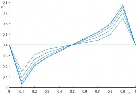
Figure 1. Function distribution graph u(x,y,t) (explicit scheme) at t=0.9 along the axis ОX at $\varepsilon=0.001$
Figure 2. Displacement changes v(x,y,t) along the axis ОX at the nodal point (y=0.6, t=0.9)
Numerical results obtained by explicit and implicit schemes were determined by recurrence relations and the elimination method, respectively. Numerical results for the component of displacement and temperature obtained by two methods for comparison are shown in Tables 1-4 and Figures 1-2. Comparing the corresponding tables for displacement u(x,y,t) and temperature T(x,y,t), and figures, one can make sure that the numerical results obtained by the two methods at t=0.9 are very close. The joint solution of the equations of thermoelasticity and thermal conductivity makes it possible to more adequately describe the process of linear and nonlinear deformation of solids under the influence of mechanical and thermal influences.
Table 1. Values of the function u(x,y,t) (explicit scheme) at t=0.9
|
|
x=0 |
x=0.1 |
x=0.2 |
x=0.3 |
x=0.4 |
x=0.5 |
x=0.6 |
x=0.7 |
x=0.8 |
x=0.9 |
x=1 |
|
y=0 |
0 |
0.0000 |
0.0000 |
0.0000 |
0.0000 |
0 |
0.0000 |
0.0000 |
0.0000 |
0.0000 |
0 |
|
y=0.1 |
0 |
-0.0499 |
-0.0185 |
-0.0082 |
-0.0040 |
0 |
0.0040 |
0.0082 |
0.0185 |
0.0499 |
0 |
|
y=0.2 |
0 |
-0.0606 |
-0.0270 |
-0.0142 |
-0.0071 |
0 |
0.0071 |
0.0142 |
0.0270 |
0.0606 |
0 |
|
y=0.3 |
0 |
-0.0686 |
-0.0340 |
-0.0192 |
-0.0098 |
0 |
0.0098 |
0.0192 |
0.0340 |
0.0686 |
0 |
|
y=0.4 |
0 |
-0.0731 |
-0.0384 |
-0.0225 |
-0.0115 |
0 |
0.0115 |
0.0225 |
0.0384 |
0.0731 |
0 |
|
y=0.5 |
0 |
-0.0747 |
-0.0399 |
-0.0236 |
-0.0121 |
0 |
0.0121 |
0.0236 |
0.0399 |
0.0747 |
0 |
|
y=0.6 |
0 |
-0.0731 |
-0.0384 |
-0.0225 |
-0.0115 |
0 |
0.0115 |
0.0225 |
0.0384 |
0.0731 |
0 |
|
y=0.7 |
0 |
-0.0686 |
-0.0340 |
-0.0192 |
-0.0098 |
0 |
0.0098 |
0.0192 |
0.0340 |
0.0686 |
0 |
|
y=0.8 |
0 |
-0.0606 |
-0.0270 |
-0.0142 |
-0.0071 |
0 |
0.0071 |
0.0142 |
0.0270 |
0.0606 |
0 |
|
y=0.9 |
0 |
-0.0499 |
-0.0185 |
-0.0082 |
-0.0040 |
0 |
0.0040 |
0.0082 |
0.0185 |
0.0499 |
0 |
|
y=1 |
0 |
0.0000 |
0.0000 |
0.0000 |
0.0000 |
0 |
0.0000 |
0.0000 |
0.0000 |
0.0000 |
0 |
Table 2. Values of the function u(x,y,t) (implicit scheme) at t=0.9
|
|
x=0 |
x=0.1 |
x=0.2 |
x=0.3 |
x=0.4 |
x=0.5 |
x=0.6 |
x=0.7 |
x=0.8 |
x=0.9 |
x=1 |
|
y=0 |
0 |
0.0000 |
0.0000 |
0.0000 |
0.0000 |
0 |
0.0000 |
0.0000 |
0.0000 |
0.0000 |
0 |
|
y=0.1 |
0 |
-0.0447 |
-0.0192 |
-0.0087 |
-0.0041 |
0 |
0.0041 |
0.0087 |
0.0192 |
0.0447 |
0 |
|
y=0.2 |
0 |
-0.0546 |
-0.0277 |
-0.0147 |
-0.0072 |
0 |
0.0072 |
0.0147 |
0.0277 |
0.0546 |
0 |
|
y=0.3 |
0 |
-0.0619 |
-0.0345 |
-0.0197 |
-0.0098 |
0 |
0.0098 |
0.0197 |
0.0345 |
0.0619 |
0 |
|
y=0.4 |
0 |
-0.0661 |
-0.0388 |
-0.0229 |
-0.0115 |
0 |
0.0115 |
0.0229 |
0.0388 |
0.0661 |
0 |
|
y=0.5 |
0 |
-0.0675 |
-0.0403 |
-0.0240 |
-0.0121 |
0 |
0.0121 |
0.0240 |
0.0403 |
0.0675 |
0 |
|
y=0.6 |
0 |
-0.0661 |
-0.0388 |
-0.0229 |
-0.0115 |
0 |
0.0115 |
0.0229 |
0.0388 |
0.0661 |
0 |
|
y=0.7 |
0 |
-0.0619 |
-0.0345 |
-0.0197 |
-0.0098 |
0 |
0.0098 |
0.0197 |
0.0345 |
0.0619 |
0 |
|
y=0.8 |
0 |
-0.0546 |
-0.0277 |
-0.0147 |
-0.0072 |
0 |
0.0072 |
0.0147 |
0.0277 |
0.0546 |
0 |
|
y=0.9 |
0 |
-0.0447 |
-0.0192 |
-0.0087 |
-0.0041 |
0 |
0.0041 |
0.0087 |
0.0192 |
0.0447 |
0 |
|
y=1 |
0 |
0.0000 |
0.0000 |
0.0000 |
0.0000 |
0 |
0.0000 |
0.0000 |
0.0000 |
0.0000 |
0 |
Table 3. Values of the function T(x,y,t) (explicit scheme) at t=0.9
|
|
x=0 |
x=0.1 |
x=0.2 |
x=0.3 |
x=0.4 |
x=0.5 |
x=0.6 |
x=0.7 |
x=0.8 |
x=0.9 |
x=1 |
|
y=0 |
0 |
0.0000 |
0.0000 |
0.0000 |
0.0000 |
0.0000 |
0.0000 |
0.0000 |
0.0000 |
0.0000 |
0 |
|
y=0.1 |
0 |
12.9459 |
15.5948 |
16.8111 |
17.5024 |
17.7311 |
0.0040 |
0.0082 |
0.0185 |
0.0499 |
0 |
|
y=0.2 |
0 |
15.5948 |
19.3707 |
21.4371 |
22.6623 |
23.0720 |
0.0071 |
0.0142 |
0.0270 |
0.0606 |
0 |
|
y=0.3 |
0 |
16.8111 |
21.4371 |
24.2105 |
25.8822 |
26.4439 |
0.0098 |
0.0192 |
0.0340 |
0.0686 |
0 |
|
y=0.4 |
0 |
17.5024 |
22.6623 |
25.8822 |
27.8386 |
28.4974 |
0.0115 |
0.0225 |
0.0384 |
0.0731 |
0 |
|
y=0.5 |
0 |
17.7311 |
23.0720 |
26.4439 |
28.4974 |
29.1893 |
0.0121 |
0.0236 |
0.0399 |
0.0747 |
0 |
|
y=0.6 |
0 |
17.5024 |
22.6623 |
25.8822 |
27.8386 |
28.4974 |
0.0115 |
0.0225 |
0.0384 |
0.0731 |
0 |
|
y=0.7 |
0 |
16.8111 |
21.4371 |
24.2105 |
25.8822 |
26.4439 |
0.0098 |
0.0192 |
0.0340 |
0.0686 |
0 |
|
y=0.8 |
0 |
15.5948 |
19.3707 |
21.4371 |
22.6623 |
23.0720 |
0.0071 |
0.0142 |
0.0270 |
0.0606 |
0 |
|
y=0.9 |
0 |
12.9459 |
15.5948 |
16.8111 |
17.5024 |
17.7311 |
0.0040 |
0.0082 |
0.0185 |
0.0499 |
0 |
|
y=1 |
0 |
0.0000 |
0.0000 |
0.0000 |
0.0000 |
0.0000 |
0.0000 |
0.0000 |
0.0000 |
0.0000 |
0 |
Table 4. Values of the function T(x,y,t) (implicit scheme) at t=0.9
|
|
x=0 |
x=0.1 |
x=0.2 |
x=0.3 |
x=0.4 |
x=0.5 |
x=0.6 |
x=0.7 |
x=0.8 |
x=0.9 |
x=1 |
|
y=0 |
0 |
0.0000 |
0.0000 |
0.0000 |
0.0000 |
0.0000 |
0.0000 |
0.0000 |
0.0000 |
0.0000 |
0 |
|
y=0.1 |
0 |
13.0272 |
15.6158 |
16.8037 |
17.4873 |
17.7154 |
17.4873 |
16.8037 |
15.6158 |
13.0272 |
0 |
|
y=0.2 |
0 |
15.6797 |
19.5042 |
21.5686 |
22.8088 |
23.2282 |
22.8088 |
21.5686 |
19.5042 |
15.6797 |
0 |
|
y=0.3 |
0 |
16.8549 |
21.5559 |
24.3177 |
26.0055 |
26.5790 |
26.0055 |
24.3177 |
21.5559 |
16.8549 |
0 |
|
y=0.4 |
0 |
17.5352 |
22.7935 |
26.0028 |
27.9792 |
28.6524 |
27.9792 |
260028 |
22.7935 |
17.5352 |
0 |
|
y=0.5 |
0 |
17.7626 |
23.2124 |
26.5758 |
28.6518 |
29.3593 |
28.6518 |
26.5758 |
23.2124 |
17.7626 |
0 |
|
y=0.6 |
0 |
17.5352 |
22.7935 |
26.0028 |
27.9792 |
28.6524 |
27.9792 |
260028 |
22.7935 |
17.5352 |
0 |
|
y=0.7 |
0 |
16.8549 |
21.5559 |
24.3177 |
26.0055 |
26.5790 |
26.0055 |
24.3177 |
21.5559 |
16.8549 |
0 |
|
y=0.8 |
0 |
15.6797 |
19.5042 |
21.5686 |
22.8088 |
23.2282 |
22.8088 |
21.5686 |
19.5042 |
15.6797 |
0 |
|
y=0.9 |
0 |
13.0272 |
15.6158 |
16.8037 |
17.4873 |
17.7154 |
17.4873 |
16.8037 |
15.6158 |
13.0272 |
0 |
|
y=1 |
0 |
0.0000 |
0.0000 |
0.0000 |
0.0000 |
0.0000 |
0.0000 |
0.0000 |
0.0000 |
0.0000 |
0 |
The coupled boundary value problem of thermoplasticity (1-8) taking into account the Eqns. (9)-(10) may be written regarding the displacements and temperature for $\varepsilon_{u} \geq \varepsilon_{u}^{*}$, which in two-dimensional case has the form:
$(\lambda+2 \mu) \frac{\partial^{2} u}{\partial x^{2}}+(\lambda+\mu) \frac{\partial^{2} v}{\partial x \partial y}$
$+\mu \frac{\partial^{2} u}{\partial y^{2}}-\gamma \frac{\partial T}{\partial x}+X_{1}^{*}=\rho \frac{\partial^{2} u}{\partial t^{2}}$
$(\lambda+2 \mu) \frac{\partial^{2} v}{\partial y^{2}}+(\lambda+\mu) \frac{\partial^{2} u}{\partial x \partial y}$
$+\mu \frac{\partial^{2} v}{\partial x^{2}}-\gamma \frac{\partial T}{\partial y}+X_{2}^{*}=\rho \frac{\partial^{2} v}{\partial t^{2}}$. (28)
${{\lambda }_{0}}\left( \frac{{{\partial }^{2}}T}{\partial {{x}^{2}}}+\frac{{{\partial }^{2}}T}{\partial {{y}^{2}}} \right)-{{c}_{\varepsilon }}\frac{\partial T}{\partial t}-\gamma T\left( \frac{{{\partial }^{2}}u}{\partial x\partial t}+\frac{{{\partial }^{2}}v}{\partial y\partial t} \right)=0$ (29)
with corresponding initial,
${{\left. u\left( x,y,t \right) \right|}_{t=0}}={{\phi }_{1}},$ ${{\left. \frac{\partial u}{\partial t} \right|}_{t=0}}={{\psi }_{1}},$${{\left. v\left( x,y,t \right) \right|}_{t=0}}={{\phi }_{2}},$ ${{\left. \frac{\partial v}{\partial t} \right|}_{t=0}}={{\psi }_{2}},$${{\left. T\left( x,y,t \right) \right|}_{t=0}}={{T}_{0}}$ (30)
and boundary conditions,
${{\left. u\left( x,\,y,t \right) \right|}_{x=0}}={{u}_{0}},{{\left. u\left( x,y,\,t \right) \right|}_{x=\ell }}_{_{1}}={{\bar{u}}_{0}},$
${{\left. u\left( x,\,y,t \right) \right|}_{y=0}}={{{u}'}_{0}},{{\left. u\left( x,y,\,t \right) \right|}_{y={{\ell }_{2}}}}={{{\bar{u}}'}_{0}},$
${{\left. v\left( x,\,y,t \right) \right|}_{x=0}}={{v}_{0}},{{\left. v\left( x,y,\,t \right) \right|}_{x=\ell }}_{_{1}}={{\bar{v}}_{0}},$
${{\left. v\left( x,\,y,t \right) \right|}_{y=0}}={{{v}'}_{0}},{{\left. v\left( x,y,\,t \right) \right|}_{y=\ell }}_{_{2}}={{{\bar{v}}'}_{0}},$
${{\left. T\left( x,y,t \right) \right|}_{x=0}}={{T}_{1}}\left( t \right),{{\left. T\left( x,y,t \right) \right|}_{x=\ell }}_{_{1}}={{T}_{2}}\left( t \right),$
${{\left. T\left( x,y,t \right) \right|}_{y=0}}={{T}_{1}}^{\prime }\left( t \right),{{\left. T\left( x,y,t \right) \right|}_{y=\ell }}_{_{2}}={{{T}'}_{2}}\left( t \right)$ (31)
where,
$X_{1}^{*}=\left(-\frac{4}{3} \frac{\partial^{2} u}{\partial x^{2}}-\frac{1}{3} \frac{\partial^{2} v}{\partial x \partial y}-\frac{\partial^{2} u}{\partial y^{2}}\right)\left(\mu-\mu^{\prime}\right)\left(1-\frac{\varepsilon_{u}^{*}}{\varepsilon_{u}}\right)$
$X_{2}^{*}=\left(-\frac{4}{3} \frac{\partial^{2} v}{\partial y^{2}}-\frac{1}{3} \frac{\partial^{2} u}{\partial x \partial y}-\frac{\partial^{2} v}{\partial x^{2}}\right)\left(\mu-\mu^{\prime}\right)\left(1-\frac{\varepsilon_{u}^{*}}{\varepsilon_{u}}\right)$ (32)
Considering in the area $t \geq 0,0 \leq x \leq l, 0 \leq y \leq l$ three families of parallel lines $x=i h_{1}(i=\overline{0, n}), y=j h_{2}(j=\overline{0, n})$, t=kτ(k=0,1,2,...) and, replacing the derivatives in Eqns. (28)-(31) by finite-differential relations, we can find that:
$\left. \begin{align}
& (\lambda +2\mu )\frac{u_{i+1,j}^{k}-2u_{i,j}^{k}+u_{i-1,j}^{k}}{h_{1}^{2}}+(\lambda +\mu )\frac{v_{i+1,j+1}^{k}-v_{i-1,j+1}^{k}-v_{i+1,j-1}^{k}+v_{i-1,j-1}^{k}}{4{{h}_{1}}{{h}_{2}}}+ \\
& \mu \frac{u_{i,j+1}^{k}-2u_{i,j}^{k}+u_{i,j-1}^{k}}{h_{2}^{2}}-\gamma \frac{T_{i+1,j}^{k}-T_{i-1,j}^{k}}{2{{h}_{1}}}+X_{1}^{*}=\rho \frac{u_{i,j}^{k+1}-2u_{i,j}^{k}+u_{i,j}^{k-1}}{{{\tau }^{2}}} \\
& (\lambda +2\mu )\frac{v_{i,j+1}^{k}-2v_{i,j}^{k}+v_{i,j-1}^{k}}{h_{2}^{2}}+(\lambda +\mu )\frac{u_{i+1,j+1}^{k}-u_{i-1,j+1}^{k}-u_{i+1,j-1}^{k}+u_{i-1,j-1}^{k}}{4{{h}_{1}}{{h}_{2}}}+ \\
& \mu \frac{v_{i+1,j}^{k}-2v_{i,j}^{k}+v_{i-1,j}^{k}}{h_{1}^{2}}-\gamma \frac{T_{i,j+1}^{k}-T_{i,j-1}^{k}}{2{{h}_{2}}}+X_{2}^{*}=\rho \frac{v_{i,j}^{k+1}-2v_{i,j}^{k}+v_{i,j}^{k-1}}{{{\tau }^{2}}} \\
\end{align} \right\}$ (33)
$\lambda_{0}\left(\frac{T_{i+1, j}^{k}-T u_{i, j}^{k}+T_{i-1, j}^{k}}{h_{1}^{2}}+\frac{T_{i, j+1}^{k}-2 T_{i, j}^{k}+T_{i, j-1}^{k}}{h_{2}^{2}}\right)$
$-c_{\varepsilon} \frac{T_{i, j}^{k+1}-T_{i, j}^{k}}{\tau}-$
$-\gamma T_{i, j}^{k}\left(\frac{u_{i+1, j}^{k+1}-u_{i-1, j}^{k+1}-u_{i+1, j}^{k-1}+u_{i-1, j}^{k-1}}{4 h_{1} \tau}\right.$
$\left.+\frac{v_{i, j+1}^{k+1}-v_{i, j-1}^{k+1}-v_{i, j+1}^{k-1}+v_{i, j-1}^{k-1}}{4 h_{2} \tau}\right)=0$ (34)
and, having solved the differential equations regarding the $u_{i, j}^{k+1}, v_{i, j}^{k+1}, T_{i, j}^{k+1}$ respectively, by analogy to the previous section we can find,
$u_{i, j}^{k+1}=\frac{\tau^{2}}{\rho}\left((\lambda+2 \mu) \frac{u_{i+1, j}^{k}-2 u_{i, j}^{k}+u_{i-1, j}^{k}}{h_{1}^{2}}+\mu \frac{u_{i, j+1}^{k}-2 u_{i, j}^{k}+u_{i, j-1}^{k}}{h_{2}^{2}}+\right.$
$\left.+(\lambda+\mu) \frac{v_{i+1, j+1}^{k}-v_{i-1, j+1}^{k}-v_{i+1, j-1}^{k}+v_{i-1, j-1}^{k}}{4 h_{1} h_{2}}-\gamma \frac{T_{i+1, j}^{k}-T_{i-1, j}^{k}}{2 h_{1}}+X_{1}^{*}\right)+$
$+2 u_{i, j}^{k}-u_{i, j}^{k-1}$ (35)
$v_{i, j}^{k+1}=\frac{\tau^{2}}{\rho}\left((\lambda+2 \mu) \frac{v_{i, j+1}^{k}-2 v_{i, j}^{k}+u_{i, j-1}^{k}}{h_{2}^{2}}+\mu \frac{v_{i+1, j}^{k}-2 v_{i, j}^{k}+v_{i-1, j}^{k}}{h_{1}^{k}}+\right.$
$\left.+(\lambda+\mu) \frac{u_{i+1, j+1}^{k}\quad-u_{i-1, j+1}^{k}\quad-u_{i+1, j-1}^{k}\quad+u_{i-1, j-1}^{k}}{4 h h_{2}}-\gamma \frac{T_{i, j+1}^{k}\quad-T_{i, j-1}^{k}}{2 h_{2}}+X_{2}^{*}\right)+$
$+2 v_{i, j}^{k}-v_{i, j}^{k-1}$ (36)
$T_{i, j}^{k+1}=\frac{\tau}{c_{\varepsilon}}\left(\lambda_{0}\left(\frac{T_{i+1, j}^{k}-T u_{i, j}^{k}+T_{i-1, j}^{k}}{h_{1}^{2}}+\frac{T_{i, j+1}^{k}-2 T_{i, j}^{k}+T_{i, j-1}^{k}}{h_{2}^{2}}\right)-\right.$
$\left.-\gamma T_{i, j}^{k}\left(\frac{u_{i+1, j}^{k+1}-u_{t-1, j}^{k+1}-u_{i+1, j}^{k-1}+u_{i-1, j}^{k-1}}{4 h_{1} \tau}+\frac{v_{i, j+1}^{k+1}-v_{i, j-1}^{k+1}-v_{i, j+1}^{k-1}+v_{i, j-1}^{k-1}}{4 h_{2} \tau}\right)\right)+T_{i, j}^{k}$ (37)
According to initial (30) and boundary (31) conditions values of the nodal functions $u_{i, j}^{k}, v_{i, j}^{k}$ and $T_{i, j}^{k}$ are known on the initial two layers k = 0 and k = 1. Then taking into account the finite-difference analogues of initial conditions (30) from Eqns. (35)-(37) at k = 0 and k = 1 may be find the following expressions for $\varepsilon_{u} \leq \varepsilon_{u}^{*}$.
$u_{i, j}^{1}=\frac{1}{2}\left(\frac{\tau^{2}}{\rho}\left((\lambda+2 \mu) \frac{u_{i+1, j}^{0}-2 u_{i, j}^{0}+u_{i-1, j}^{0}}{h_{1}^{2}}+\mu \frac{u_{i, j+1}^{0}-2 u_{i, j}^{0}+u_{i, j-1}^{0}}{h_{2}^{2}}+\right.\right.$
$\left.+(\lambda+\mu) \frac{v_{i+1, j+1}^{0}-v_{i-1, j+1}^{0}-v_{i+1, j-1}^{0}+v_{i-1, j-1}^{0}}{4 h_{1} h_{2}}-\gamma \frac{T_{i+1, j}^{0}-T_{i-1, j}^{0}}{2 h_{1}}\right)+$
$\left.+2 u_{i, j}^{0}+2 \tau \psi_{1}\right)$ (38)
$v_{i, j}^{1}=\frac{1}{2}\left(\frac{\tau^{2}}{\rho}\left((\lambda+2 \mu) \frac{v_{i, j+1}^{0}-2 v_{i, j}^{0}+u_{i, j-1}^{0}}{h_{2}^{2}}+\mu \frac{v_{i+1, j}^{0}-2 v_{i, j}^{0}+v_{i-1, j}^{0}}{h_{1}^{2}}+\right.\right.$
$\left.+(\lambda+\mu) \frac{u_{i+1, j+1}^{0}-u_{i-1, j+1}^{0}-u_{i+1, j-1}^{0}+u_{i-1, j-1}^{0}}{4 h_{1} h_{2}}-\gamma \frac{T_{i, j+1}^{0}-T_{i, j-1}^{0}}{2 h_{2}}\right)+$
$\left.+2 v_{i, j}^{0}+2 \tau \psi_{2}\right)$ (39)
$T_{i, j}^{1}=\frac{\tau}{c_{\varepsilon}}\left(\lambda_{0}\left(\frac{T_{i+1, j}^{0}-2 T_{i, j}^{0}+T_{i-1, j}^{0}}{h_{1}^{2}}+\frac{T_{i, j+1}^{o}-2 T_{i, j}^{0}+T_{i, j-1}^{0}}{h_{2}^{2}}\right)-\right.$
$-\gamma T_{i, j}^{0}\left(\frac{u_{i+1, j}^{1}-u_{i-1, j}^{1}-u_{i+1, j}^{0}+u_{i-1, j}^{0}}{2 h_{1} \tau}+\frac{v_{i, j+1}^{1}-v_{i, j-1}^{1}-v_{i, j+1}^{0}+v_{i, j-1}^{0}}{2 h_{2} \tau}\right)+T_{i, j}^{0}$ (40)
So, finite-difference Eqns. (33-34) present an explicit scheme and can be solved using the recurrence relations (35-40) with a following thermomechanical initial,
$u_{i j}^{0}=0, \frac{u_{i j}^{1}-u_{i j}^{0}}{\tau}=0$,
$v_{i j}^{0}=0, \frac{v_{i j}^{1}-v_{i j}^{0}}{\tau}=0$,
$T_{i j}^{0}=T_{0}+T_{0} \sin \left(\frac{\pi x_{i}}{l_{1}}\right) \sin \left(\frac{\pi y_{j}}{l_{2}}\right)$,
The boundary conditions:
$u_{0 j}^{k}=0, u_{N_{1} j}^{k}=0, u_{i 0}^{k}=0, u_{i N_{2}}^{k}=0$,
$v_{0 j}^{k}=0, v_{N_{1} j}^{k}=0, v_{i 0}^{k}=0, v_{i N_{2}}^{k}=0$,
$T_{0 j}^{k}=0, T_{N_{1} j}^{k}=0, T_{i 0}^{k}=0, T_{i N_{2}}^{k}=0$.
The elastic-plastic thermo-mechanical constants were taking as following values: The numerical results of the coupled thermoelasticity problem (28-31) for displacement and temperature received by explicit and implicit schemes at time t=0.9 are shown in Tables 5-8 and they very close.
$\lambda=0.78 * 10^{5} \mathrm{~kg} / \mathrm{sm}^{2}, \alpha=0.05 * 10^{-5}, \mu=0.7 *$
$10^{5} \mathrm{~kg} / \mathrm{sm}^{2}, \rho=0.86 * 10^{4} \mathrm{~kg} / \mathrm{m}^{3}, c_{\varepsilon}=3.4 * 10^{4} J /(\mathrm{kg} *$
$K), T_{0}=15^{0} \mathrm{C}, \lambda_{0}=0.06, \mu^{\prime}=0.4 * 10^{5} \mathrm{~kg} / \mathrm{sm}^{2}, h_{1}=0.1$
$h_{2}=0.1, \tau=0.01, \ell_{i}=1, n_{1}=n_{2}=10$.
Table 5. Values of the function u(x,y,t) (explicit scheme) at t=0.9
|
|
x=0 |
x=0.1 |
x=0.2 |
x=0.3 |
x=0.4 |
x=0.5 |
x=0.6 |
x=0.7 |
x=0.8 |
x=0.9 |
x=1 |
|
y=0 |
0 |
0.0000 |
0.0000 |
0.0000 |
0.0000 |
0 |
0.0000 |
0.0000 |
0.0000 |
0.0000 |
0 |
|
y=0.1 |
0 |
-0.0513 |
-0.0185 |
-0.0082 |
-0.0040 |
0 |
0.0040 |
0.0082 |
0.0185 |
0.0513 |
0 |
|
y=0.2 |
0 |
-0.0610 |
-0.0270 |
-0.0142 |
-0.0071 |
0 |
0.0071 |
0.0142 |
0.0270 |
0.0610 |
0 |
|
y=0.3 |
0 |
-0.0687 |
-0.0340 |
-0.0192 |
-0.0098 |
0 |
0.0098 |
0.0192 |
0.0340 |
0.0687 |
0 |
|
y=0.4 |
0 |
-0.0732 |
-0.0384 |
-0.0225 |
-0.0115 |
0 |
0.0115 |
0.0225 |
0.0384 |
0.0732 |
0 |
|
y=0.5 |
0 |
-0.0747 |
-0.0399 |
-0.0236 |
-0.0121 |
0 |
0.0121 |
0.0236 |
0.0399 |
0.0747 |
0 |
|
y=0.6 |
0 |
-0.0732 |
-0.0384 |
-0.0225 |
-0.0115 |
0 |
0.0115 |
0.0225 |
0.0384 |
0.0732 |
0 |
|
y=0.7 |
0 |
-0.0687 |
-0.0340 |
-0.0192 |
-0.0098 |
0 |
0.0098 |
0.0192 |
0.0340 |
0.0687 |
0 |
|
y=0.8 |
0 |
-0.0610 |
-0.0270 |
-0.0142 |
-0.0071 |
0 |
0.0071 |
0.0142 |
0.0270 |
0.0610 |
0 |
|
y=0.9 |
0 |
-0.0513 |
-0.0185 |
-0.0082 |
-0.0040 |
0 |
0.0040 |
0.0082 |
0.0185 |
0.0513 |
0 |
|
y=1 |
0 |
0.0000 |
0.0000 |
0.0000 |
0.0000 |
0 |
0.0000 |
0.0000 |
0.0000 |
0.0000 |
0 |
Table 6. Values of the function u(x,y,t) (implicit scheme) at t=0.9
|
|
x=0 |
x=0.1 |
x=0.2 |
x=0.3 |
x=0.4 |
x=0.5 |
x=0.6 |
x=0.7 |
x=0.8 |
x=0.9 |
x=1 |
|
y=0 |
0 |
0.0000 |
0.0000 |
0.0000 |
0.0000 |
0 |
0.0000 |
0.0000 |
0.0000 |
0.0000 |
0 |
|
y=0.1 |
0 |
-0.0438 |
-0.0192 |
-0.0087 |
-0.0041 |
0 |
0.0041 |
0.0087 |
0.0192 |
0.0438 |
0 |
|
y=0.2 |
0 |
-0.0542 |
-0.0277 |
-0.0147 |
-0.0072 |
0 |
0.0072 |
0.0147 |
0.0277 |
0.0542 |
0 |
|
y=0.3 |
0 |
-0.0618 |
-0.0345 |
-0.0197 |
-0.0098 |
0 |
0.0098 |
0.0197 |
0.0345 |
0.0618 |
0 |
|
y=0.4 |
0 |
-0.0661 |
-0.0388 |
-0.0229 |
-0.0115 |
0 |
0.0115 |
0.0229 |
0.0388 |
0.0661 |
0 |
|
y=0.5 |
0 |
-0.0675 |
-0.0403 |
-0.0240 |
-0.0121 |
0 |
0.0121 |
0.0240 |
0.0403 |
0.0675 |
0 |
|
y=0.6 |
0 |
-0.0661 |
-0.0388 |
-0.0229 |
-0.0115 |
0 |
0.0115 |
0.0229 |
0.0388 |
0.0661 |
0 |
|
y=0.7 |
0 |
-0.0618 |
-0.0345 |
-0.0197 |
-0.0098 |
0 |
0.0098 |
0.0197 |
0.0345 |
0.0618 |
0 |
|
y=0.8 |
0 |
-0.0542 |
-0.0277 |
-0.0147 |
-0.0072 |
0 |
0.0072 |
0.0147 |
0.0277 |
0.0542 |
0 |
|
y=0.9 |
0 |
-0.0438 |
-0.0192 |
-0.0087 |
-0.0041 |
0 |
0.0041 |
0.0087 |
0.0192 |
0.0438 |
0 |
|
y=1 |
0 |
0.0000 |
0.0000 |
0.0000 |
0.0000 |
0 |
0.0000 |
0.0000 |
0.0000 |
0.0000 |
0 |
Table 7. Values of the function εu (explicit scheme) at t=0.9
|
|
x=0 |
x=0.1 |
x=0.2 |
x=0.3 |
x=0.4 |
x=0.5 |
x=0.6 |
x=0.7 |
x=0.8 |
x=0.9 |
x=1 |
|
y=0 |
0 |
0.0000 |
0.0000 |
0.0000 |
0.0000 |
0 |
0.0000 |
0.0000 |
0.0000 |
0.0000 |
0 |
|
y=0.1 |
0 |
0.3526 |
0.2494 |
0.1783 |
0.1565 |
0.1548 |
0.1565 |
0.1783 |
0.2494 |
0.3526 |
0 |
|
y=0.2 |
0 |
0.2494 |
0.1284 |
0.1219 |
0.1224 |
0.1186 |
0.1224 |
0.1219 |
0.1284 |
0.2494 |
0 |
|
y=0.3 |
0 |
0.1783 |
0.1219 |
0.0728 |
0.0616 |
0.0485 |
0.0616 |
0.0728 |
0.1219 |
0.1783 |
0 |
|
y=0.4 |
0 |
0.1565 |
0.1224 |
0.0616 |
0.0485 |
0.0479 |
0.0485 |
0.0616 |
0.1224 |
0.1565 |
0 |
|
y=0.5 |
0 |
0.1548 |
0.1186 |
0.0578 |
0.0479 |
0.0492 |
0.0479 |
0.0578 |
0.1186 |
0.1548 |
0 |
|
y=0.6 |
0 |
0.1565 |
0.1224 |
0.0616 |
0.0485 |
0.0479 |
0.0485 |
0.0616 |
0.1224 |
0.1565 |
0 |
|
y=0.7 |
0 |
0.1783 |
0.1219 |
0.0728 |
0.0616 |
0.0485 |
0.0616 |
0.0728 |
0.1219 |
0.1783 |
0 |
|
y=0.8 |
0 |
0.2494 |
0.1284 |
0.1219 |
0.1224 |
0.1186 |
0.1224 |
0.1219 |
0.1284 |
0.2494 |
0 |
|
y=0.9 |
0 |
0.3526 |
0.2494 |
0.1783 |
0.1565 |
0.1548 |
0.1565 |
0.1783 |
0.2494 |
0.3526 |
0 |
|
y=1 |
0 |
0.0000 |
0.0000 |
0.0000 |
0.0000 |
0 |
0.0000 |
0.0000 |
0.0000 |
0.0000 |
0 |
Table 8. Values of the function εu (implicit scheme) at t=0.9
|
|
x=0 |
x=0.1 |
x=0.2 |
x=0.3 |
x=0.4 |
x=0.5 |
x=0.6 |
x=0.7 |
x=0.8 |
x=0.9 |
x=1 |
|
y=0 |
0 |
0.0000 |
0.0000 |
0.0000 |
0.0000 |
0.0000 |
0.0000 |
0.0000 |
0.0000 |
0.0000 |
0 |
|
y=0.1 |
0 |
0.3178 |
0.2339 |
0.1785 |
0.1579 |
0.1553 |
0.1579 |
0.1785 |
0.2339 |
0.3178 |
0 |
|
y=0.2 |
0 |
0.2342 |
0.1189 |
0.1048 |
0.0995 |
0.0575 |
0.0995 |
0.1048 |
0.1189 |
0.2342 |
0 |
|
y=0.3 |
0 |
0.1785 |
0.1046 |
0.0722 |
0.0611 |
0.0575 |
0.0611 |
0.0722 |
0.1046 |
0.1785 |
0 |
|
y=0.4 |
0 |
0.1577 |
0.0994 |
0.0610 |
0.0495 |
0.0486 |
0.0495 |
0.0610 |
0.0994 |
0.1577 |
0 |
|
y=0.5 |
0 |
0.0000 |
0.1550 |
0.0950 |
0.0573 |
0.0486 |
0.0495 |
0.0486 |
0.0573 |
0.1550 |
0 |
|
y=0.6 |
0 |
0.1577 |
0.0994 |
0.0610 |
0.0495 |
0.0486 |
0.0495 |
0.0610 |
0.0994 |
0.1577 |
0 |
|
y=0.7 |
0 |
0.1785 |
0.1046 |
0.0722 |
0.0611 |
0.0575 |
0.0611 |
0.0722 |
0.1046 |
0.1785 |
0 |
|
y=0.8 |
0 |
0.2342 |
0.1189 |
0.1048 |
0.0995 |
0.0575 |
0.0995 |
0.1048 |
0.1189 |
0.2342 |
0 |
|
y=0.9 |
0 |
0.3178 |
0.2339 |
0.1785 |
0.1579 |
0.1553 |
0.1579 |
0.1785 |
0.2339 |
0.3178 |
0 |
|
y=1 |
0 |
0.0000 |
0.0000 |
0.0000 |
0.0000 |
0.0000 |
0.0000 |
0.0000 |
0.0000 |
0.0000 |
0 |
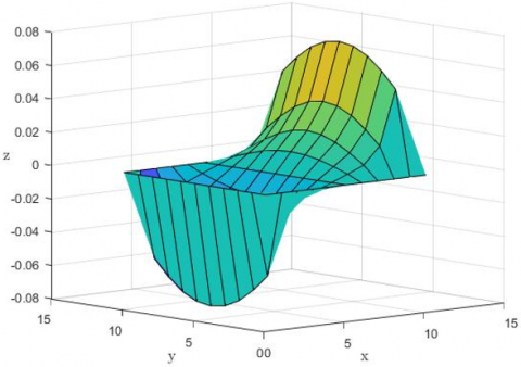
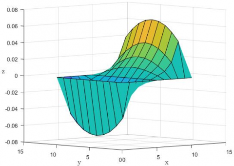
Figure 3. Distribution of the displacement u(x,y,t) (explicit scheme) at t=0.9 and ε=0.001
Figure 4. Distribution of the displacement u(x,y,t) (implicit scheme) at t=0.9 and ε=0.001
Figure 5. Displacement changings u(x,y,t) along the axis ОZ at the nodal point (x=0.5, y=0.7)
In Figures 3 and 4 the distribution of displacements u(x,y,t) received by the implicit and explicit schemes is compared. In Figure 5 the coincidence of the curves received implicit and explicit schemes are shown.
The coupled dynamic thermoelasticity and thermoplasticity boundary value problems are formulated. The coupled thermoplasticity problem is based on deformation theory of plasticity. The thermo-elastic-plastic boundary value problems for rectangle in different initial and boundary conditions are considered. Discrete equations are compiled by the finite-differential method in the form of explicit and implicit schemes. The solution of the explicit schemes is reduced to the recurrence relations regarding the displacement components and temperature. Implicit schemes are solved using the elimination method along the corresponding directions.
Effective numerical algorithm and corresponding software for solving two-dimensional thermo-elasto-plastic boundary value problems have been developed. A number of thermo-elasto-plastic problems on clamped from all sides rectangle with a given temperature field, have been solved. The obtained numerical results by different methods are compared and received a close coincidence. The influence of the temperature field on the displacement distribution and, as well as on the appearance of plastic zones in a rectangle, has been investigated.
[1] Ilyushin A.A. (1948). Plastic. Part 1. Elastoplastic deformations. Gostekhizdat, Moscow [in Russian].
[2] Biot, M.A. (1956). Thermoelasticity and irreversible thermodynamics. Journal of Applied Physics, 27(3): 240-253. https://doi.org/10.1063/1.1722351
[3] Kachanov, L.M. (1969). Fundamentals of the Theory of Plasticity. M: Nauka.
[4] Novatski, V.V. (1975). Theory of Elasticity. M: Mir, p872.
[5] Pobedrya, B.E. (1984). Deformation theory of plasticity of anisotropic media. Journal of Applied Mathematics and Mechanics, 48(1): 10-17. https://doi.org/10.1016/0021-8928(84)90100-X
[6] Khaldjigitov, A.A. (1998). On the equations of thermoplasticity. The Problem of Mechanics, 1: 31-34.
[7] Khaldjigitov, A.A., Long, N.M.A.N., Qalandarov, A., Eshkuvatov, Z.K. (2014). Mathematical and numerical modelling of the thermoplastic coupled problem. In International Conference on Mathematical Sciences and Statistics, 2013: 69-75. https://doi.org/10.1007/978-981-4585-33-0_8
[8] Khaldjigitov, A.A., Babajanov, M.R., Kalandarov, А.A., Khudazarov, R.S. (2020). Coupled dynamic thermoplasticity problem for transversely isotropic parallelepiped. International Journal, 8(7): 3958-3964. https://doi.org/10.30534/ijeter/2020/166872020
[9] Khaldjigitov, A.A., Adambaev, U.E., Babajanov, M.R. (2019). Finite-difference method for solving elastoplastic problems of anisotropic bodies. Applied Mathematics and Control Issues, 4: 9-25.
[10] Khaldjigitov, A.A., Kalandarov, A.A, Yusupov, S. (2019). Coupled problems of thermoelasticity and thermoplasticity. -T.:"Fan va texnologiya", 203. (In Russian)
[11] Khaldjigitov, A.A., Khudazarov, R.S., Sagdullayeva, D.A. (2015). The theory of plasticity and thermoplasticity of anisotropic bodies. -T.:"Fan va texnologiya ", 320. (in Russian).
[12] Kalandarov, A.A., Adambaev, U.E., Kalandarov, A. (2017). Coupled thermoelasticity problem for an isotropic parallelepiped. Bulletin of NUUZ, Exact Sciences, 2(1): 92-99.
[13] Kalandarov A.A, Adambaev U.E, Khudazarov R.S. (2010). Coupled and uncoupled problemas of thermoelastoplasticity. Bulletin of NUUZ, 2010 3: 92-95.
[14] Khaldjigitov, A.A., Yusupov, Y.S., Rasedee, A.F.N., Nik Long, N.M.A. (2019). Mathematical modeling and simulation of the coupled strain space thermoplasticity problems. Journal of physics: Conference series, 1212(1): 1-12. https://doi.org/10.1088/1742-6596/1212/1/012023
[15] Yusupov, Y.S., Babadjanov, M.R. (2019). Numerical solution of a three-dimensional coupled thermoplastic problem based on deformation theory. The International Journal of Science & Technoledge, 7(9): 23-35. https://doi.org/10.24940/theijst/2019/v7/i9/ST1909-012
[16] Yusupov, Y., Khaldjigitov, A.A. (2017). Mathematical and numerical modeling of the coupled dynamic thermoplastic problem. Universal Journal of Computational Mathematics, 5(2): 34-43. https://doi.org/10.13189/ujcmj.2017.050204
[17] Long, N.N., Khaldjigitov, A.A., Adambaev, U. (2013). On the constitutive relations for isotropic and transversely isotropic materials. Applied Mathematical Modelling, 37(14-15): 7726-7740. https://doi.org/10.1016/j.apm.2013.03.012
[18] Khaldjigitov, A.A., Djumayozov, U.Z., Ibodulloev, S.R. (2020). Effective finite-difference method for elastoplastic boundary value problems. AIP Conference Proceedings, 2365(1): 020008. https://doi.org/10.1063/5.0057047
[19] Abirov, R.A., Khusanov, B.E., Sagdullaeva, D.A. (2020). Numerical modeling of the problem of indentation of elastic and elastic-plastic massive bodies. In IOP Conference Series: Materials Science and Engineering, 971(3): 032017. https://doi.org/10.1088/1757-899X/971/3/032017
[20] Kalandarov, A.A., Khaldjigitov, A.A. (2019). Computer simulation of the coupled dynamic thermoelasticity problem for a two-dimensional isotropic bodies. The International Journal of Science and Technoledge, 7(5): 24-32.
[21] Khaldjigitov, A., Qalandarov, A., Nik Long, N.M.A., Eshquvatov, Z. (2012). Numerical solution of 1D and 2D thermoelastic coupled problems. In International Journal of Modern Physics: Conference Series, 9: 503-510. https://doi.org/10.1142/S2010194512005594
[22] Qalandarov, A.A., Khaldjigitov, A.A. (2020). Mathematical and numerical modeling of the coupled dynamic thermoelastic problems for isotropic bodies. TWMS Journal of Pure and Applied Mathematics, 11(1): 119-126.
[23] Kalandarov, A.A., Babadjanov, M.R. (2019). Numerical simulation of the coupled dynamic thermoelastic problem for orthotropic bodies. International journal of computer science and Mobile computing, 8(9): 182-189.
[24] Khaldjigitov, A.A., Djumayozov, U.Z., Alisherov, A.A. (2020). A simple iterative method for finite difference equations of applied problems. International Conference on Recent Advances in Applied Mathematics, pp. 4-6. https://einspem.upm.edu.my/icraam2020/programme_and_abstracts_book.pdf.
[25] Jabbari, M., Dehbani, H., Eslami, M.R. (2011). An exact solution for classic coupled thermoelasticity in cylindrical coordinates. ASME. J. Pressure Vessel Technol., 133(5): 051204. https://doi.org/10.1115/1.4003459
[26] Samarski, A.A., Nikolaev, E.S. (1978). Methods for Solving Grid Equations. Science, p. 592. Nauka, Moscow. http://samarskii.ru/books/book1978.pdf.