Salah A. Adnan* | Ahmed Alchalaby | Hassan Ahmed Hassan
© 2021 IIETA. This article is published by IIETA and is licensed under the CC BY 4.0 license (http://creativecommons.org/licenses/by/4.0/).
OPEN ACCESS
Underwater Optical Wireless Communication (UWOC) becomes an emerging underwater communication technology, with high-data rates over relatively medium transmission ranges. When optical wireless signal transmitted in ocean water channel, it will suffer from drastic scattering and absorption due to water molecules, dissolved particles, air bubbles, and turbulence. Absorption and scattering of the transmitted wireless optical signal in underwater channel led to attenuation in optical signal power. Optical signal attenuation over underwater channel is an aggregate of` different parameters effects that changed frequently, then practical measuring of this attenuation is complicated, difficult, expensive, and time-consuming process. In this work, improved neural network optimized with future search algorithm (FANN) was proposed, as an efficacious solution to obtain an accurate, relabel values of attenuation coefficient in different water types and conditions. The proposed FANN model provides a good much results to the practical measured values. The performance of the proposed FANN model was evaluated using mean square error (MSE), root mean square error (RMSE) and mean absolute error (MAE) error indices. The errors in attenuation coefficient values obtained by the proposed FANN model had been calculated and its values are very acceptable which are lie lower than 10-4. The performance of the proposed FANN model shows excellent results which indicate the superior performance of the proposed FANN model.
attenuation coefficients, ANN, classified ocean water, optimization, UWOC
Our world is mostly water-covered, so data-transmission techniques among underwater devices are crucial, and a large number of applications rely on this technology [1]. Many overseas information is currently transmitted through a worldwide underwater fiber optic cable network. Such fiber optic-cables connected all continents of the world and helped make the world a small village, but in many cases, the considerable costs and restricted cable installation handling could make it difficult to use fiber optic-cables, requiring a flexible network with high ability to maneuverability [2]. The growing amount of human underwater operations raises the requirement for efficient and convenient systems and equipment to monitor and transmit information in real-time [1].
Acoustic waves for a long time considered as the most effective method of communication in underwater applications [3]. The acoustic channel bandwidth is, however, limited to several hundreds of kHz [4]. Owing to the conductivity of seawater at radio frequencies, radio-frequency communication for the long-distance transmission is extremely limited [3]. The UWOC became popular in the military and scientific research and has been suggested as an alternate or hybrid method with acoustic or radio-frequency for underwater communication channels [1].
In recent years, increasing use of UWOC have been witnessing due to its high data transmission rates, adequate information security, lower channel delay compared to acoustic and RF, and the costs of deploying, which is also lower than acoustic and RF [3].
UWOC refers to data transfer in untraced water media without optical carrier [5]. The absorption of water and small particles dissolved in it generate scattering are impact wireless optical signals [6]. The properties of the UWOC are ideal for low-range communication systems due to the water turbulence, air bubbles, scattering, and absorption that affect optical channel properties [2]. The salinity of the water has a significant impact on ocean water turbulence, absorption, and scattering. Frequent measurement of turbulence, air bubbles, scattering, and absorption effects on a laser beam is a very complex, complicated, time consuming and expensive procedure, involving accurate monitoring and measuring to these parameters’ effects. This research focuses on the estimation of 532 nm laser beam attenuation coefficient when passing through different ocean water types in different conditions.
Artificial Neural Network (ANN) has key features which are reliability, competence, and ability to simplify and find solutions related to pattern recognitions [7].
ANN 's effectiveness depends primarily on its architecture, the algorithm used for training, and the selection of the structures used in the training process [8]. The ANN is valid for numerous optimizations, as well as for math problems like recognition, artifacts and image identification, signal processing, prediction of seismic disasters, weather, bankruptcies, tsunami strength, virus spread pattern, etc. [9], [10-12]. In the past, various techniques have been used to improve ANN training efficiency, such as back propagation-neural network algorithm (BPNNA) [13]. Many optimized numerical methods have been used over the past few years to boost back propagation algorithm effectiveness [7]. Such algorithms are hybrid particle swarm algorithm-back propagation, algorithm of artificial bee colony, evolutionary algorithm, genetic algorithms, and tabu search algorithm [8], [10, 14, 15].
This paper proposes a metaheuristic search algorithm which is Future Search Algorithm (FSA) to optimize and overcome the limitation of conventional ANN. The core concept of (FSA) imitates people's actions for finding the best life [16]. The FSA develops the random initial and using local search for multi-agents and global search for the best agents in history to find the optimum solutions. The FSA is faster than other methods like genetic algorithm, firefly algorithm, and the lightning search algorithm for the most benchmark functions of the [16, 17]. Furthermore, the FSA achieved better performance among the mentioned algorithms.
The remainder of the paper is organized as follows: Section 2 includes UWOC literature reviews. Section 3, ANN is clarified. Section 4 provides analysis of the potential algorithm. The formulation of the optimum ANN problem is presented in Section 5. Section 6 described the FSA implementation based optimum ANN. The results are presented in Section 7. Eventually, the article in Section 8 was concluded.
The key drawback of UWOC is that water is an ambient that strongly absorbs the optic beam, and the second downside is the optical scattering due to dissolved detritus in seawater [3]. The absorption of the visible light spectrum in seawater, particularly in the blue-green region, is lower than that of another light spectrum [18, 19]. By Using this physical characteristic, high-speed communications can be accomplished with signals of wavelengths from the blue-green region of the spectrum according to water type [19]. In the clear water, lowest attenuation accomplished at 460 nm, but in polluted waters, it shifts to higher values to about 540 nm [20]. Oceans water optical properties are classified into inherent optical characteristics and apparent optical characteristics [2]. Inherent characteristics may be illustrated as optical parameters depending solely on the medium, i.e., on the composition of ocean water, not depending on the light source characteristics [21]. The main inherent properties of water are absorption, scattering, and volume scattering [20]. Apparent optical properties are optical parameters that not only depend on medium but also on medium and geometric structures, such as collimation and diffusion, of the transmitted light [21]. The attenuation coefficient $(\mathrm{C} \lambda)$ describes the overall attenuation effects of absorption coefficient $(\mathrm{A} \lambda)$ and scattering coefficient $(\mathrm{B} \lambda)$ of the light beam transmitted underwater, which expressed as [19]:
$\mathrm{C}_{\lambda}=\mathrm{A}_{\lambda}+B_{\lambda}$ (1)
The absorption coefficient of light beam transmitted underwater expressed as follows [22]:
$A_{(\lambda)}=A_{\omega(\lambda)}+A_{C D O M(\lambda)}+A_{P H Y T(\lambda)}+A_{D E T R(\lambda)}$ (2)
where, Aω(λ) represents light absorption caused by pure seawater, ACDOM(λ) denotes light absorption caused by CDOM, APHYT(λ) is the absorption caused by phytoplankton, and ADETR(λ) is light absorption caused by detritus.
The scattering coefficient of light beam transmitted underwater could be expressed as a summation of scattering caused by pure seawater, phytoplankton, and detritus as shown in the flowing equation [2]:
$B_{(\lambda)}=B_{\omega(\lambda)}+B_{P H Y T(\lambda)}+B_{D E T R(\lambda)}$ (3)
where, Bω(λ) represents light scattering caused by pure seawater, APHYT(λ) is the scattering caused by phytoplankton, and APHYT(λ) denotes scattering caused by detritus.
Related on attenuation coefficient, Beer-Lambert law presents the simplest and most commonly used expression to describe light beam attenuation in the underwater ambient, where the received power of underwater transmitted light after distance Z could be calculated as [3]:
$I=I_{0} e^{-C_{\lambda} Z}$ (4)
where power of transmitted light beam represented by I0, distance of transmitted denoted by Z.
In 1968, Jerlov classified ocean water types according to optical properties into ten different types (I, IA, IB, II, III,1C, 3C, 5C, 7C, and 9C) [23]. Jerlov classification has the benefit of being associated with components of ocean waters that contribute significantly to the optical properties of the ocean [24]. Jerlov water classification become generally used to classify natural water bodies [25].
The ANN was fundamentally inspired by biological neural networks which are extensively parallel processing systems comprising an incredibly large set of simple computing elements with multiple interconnections, called nodes or neuron, that are set up regularly [26]. Every node is connected by a strong connection relation to the others nodes. Every connection is incorporated with certain weights that contain data related to the input signal [27]. The neural net uses this type of data to solve different problem [27]. ANN core features are versatility, aptitude, and ability to optimize and address the problems in pattern classification, function estimation, pattern consistency and associated memory [28]. ANN has the capacity to infer unpredictable nonlinear functions and data processing that other methods do not own [8]. The BPNNA was used for ANN training for optimum network performance [29]. By measuring output layer errors, BPNNA can find errors in hidden layers [13]. According to this back propagating ability, it is appropriate for problems where output and input are not interdependent. The method of gradient descent is used to compute weights and to minimize output error [14]. The BPNNA used for multi-layer perception training [30]. BPNNA is a generalized least-mean-square algorithm minimizes sum of errors between both the actual outputs and the desired one [27].
$E_{\text {Paatern }}=\sum_{i=1}^{n}\left(E_{i}\right)^{2}$ (5)
$E_{i}=d_{i}-c_{i}$ (6)
where, di is desired output, ci is actual output, n is the output units’ number. gradient descent method is set by [7];
$w_{g i}=-\mu \frac{\partial E_{\text {Paatern }}}{\partial w_{g i}}$ (7)
where, wgi denote the weight of the i unit in the (n-1) layer to the g unit in the n layer. The Back propagation calculating errors at the output and hidden layers using the flowing in equations [7]:
$\partial_{o}=\mu\left(d_{i}-c_{i}\right) f^{\prime}\left(c_{i}\right)$ (8)
$\partial_{h}=\mu \sum_{i} \partial_{o} w_{o h} f^{\prime}\left(c_{i}\right)$ (9)
Back propagation errors are hired to update both weights and biases in output layer and hidden layer [29].
$w_{i n}(k+1)=w_{i n}(k)+\mu d_{h} c_{i}$ (10)
$w_{o h}(k+1)=w_{o h}(k)+\mu d_{h} x_{o}$ (11)
$b_{i}(k+1)=b_{i}(k)+\mu d_{h}$ (12)
The weights, win and biases bi, are adjusted by using the above equations. The number of the epoch is denoting by k and the learning rate denote by m. The key drawbacks of the BPNNA are poor convergence and volatility [28]. Drawbacks of BPNNA are due to the possibility of being trapped at local minimum and the minimums surface errors overshooting probability [31]. A number of developed algorithms were adopted recently in effort to improve performance and to overcome the limitation of conventional BPNNA [13]. Many algorithms have been mentioned in the literature such as particle swarm algorithm, artificial bee colony algorithm, evolutionary algorithms, differential evolution, ant colony, bat algorithm, and cuckoo search algorithm. In this paper a new meta-heuristic algorithm called future search algorithm (FSA) will be developed to enhance the performance of the conventional ANN.
Most fields require meta-heuristic algorithm (MHA) in the current era to acquire unbeknown parameters [28]. The MHA minimize exertion, time, errors and provide acceptable results for unknown parameter optimization compared to conventional methods, such as trial and error technique and methods dependence on designer experience [26].
The FSA simulates a people when they search for a better life. Therefore, this behaver is used in the FSA to search for the best solutions. Most of the optimization algorithms start by initializing the populations randomly [8]. This process may take the algorithm far from the global solutions and take long iterations to reach for the optimum solutions [8]. The FSA handles this drawback by update random initial during each iteration. Therefore, the FSA is faster than many other algorithms. Most of the optimization algorithms used local solution or global solution to update the populations in the next iteration which may take large iterations to find the best solutions [29]. Unlike the other optimization algorithms, The FSA overcomes the above problems by updating local solutions for each iteration and prefers the best solution overall for which the global solution has been considered [16]. The FSA will be updating the random initial and constructing its iterations to reach the best possible solutions based on local solutions and global solutions [16]. The FSA has been modeled based on simple equations unlike most of the other optimization algorithms. This leads to less time and a smaller number of iterations to reach for best solutions. In FSA, the term of local solution is modeled by the best performance of a person in a country. Meanwhile, the global solution has been modeled by the best performance of a person in a country over some years.
The process of the proposed FSA is starts by generation of the initial populations which are derived as:
$S(i,:)=L b+(U b-L b) . * \operatorname{rand}(1, d)$ (13)
where, S is the solutions, Lb and Ub are the lower and upper band, rand is random value between 0 and 1, and d is the dimensions of the problem.
Each population represents local solution (LS), meanwhile the global solution (GS) is the best of them. The exploitation is supported by the LS and it is expressed as:
$S(i,:)_{L}=(L S(i,:)-S(i,:)) * \text { rand }$ (14)
The global solution is supported exploration characteristic and defined as:
$S(i,:)_{G}=(G S-S(i,:)) * \text { rand }$ (15)
The solution of each person is defined by adding the local solution and global solution as can be defined as:
$S(i,:)=S(i,:)+S(i,:)_{L}+S(i,:)_{G}$ (16)
Finally, the random initial is updated based on GS and LS. This feature improves the exploration characteristics of the FSA and it is expressed as:
$S(i,:)=G S+(G S-L S(i,:)) * \text { rand }$ (17)
In each optimization problem, three components should be considered which are dimension of the problem, cost function formulation and constraint of the problem parameters.
5.1 Dimension of the problem
The dimension of the problem is the number of the variables that should be found by the optimization algorithms. These variables are represented by solution vector. This vector is defined as:
$D_{i, j}=\left[S_{i, j}^{1} S_{i, j}^{2} \ldots S_{i, j}^{p}\right]$ (18)
where, Di,j is the jth solution in the population during the ith iteration, $S_{i, j}^{k}$ is the kth element of Di,j, and p is the number of variables.
5.2 Cost function
The cost function is very important to assess the performance of the dimension vector Di,j. The cost function has been formulated in such a way that the dimension vector achieves the global best solution.
Three types of functions have been used in this work. These functions are mean square error (MSE), root mean square error (RMSE) and mean absolute error (MAE). These functions are expressed as:
$M S E=\frac{\sum_{i=1}^{\ell}\left(M_{\text {ref }}-M_{d}\right)^{2}}{\ell}$ (19)
$R M S E=\sqrt{\frac{\sum_{i=1}^{\ell}\left(M_{\text {ref }}-M_{d}\right)^{2}}{\ell}}$ (20)
$M S E=\frac{\sum_{i=1}^{\ell}\left|M_{r e f}-M_{d}\right|}{\ell}$ (21)
5.3 Variables constraints
The FSA find the optimum values of the variables while satisfy all constraints. The variables have the upper band and lower band. Theses boundaries should not overlap. If any variable exceeds the lower or upper band it will regenerated within the boundaries. The restrictions are described as:
$L B^{k}<S_{i, j}^{k}<U B^{k}$ (22)
In this work, the FSA has been proposed to optimize and overcome the limitation of conventional ANN. The optimum ANN has been proposed to obtain an accurate, relabel values of attenuation coefficient in different water types and conditions.
The FSA is started by define no. of iteration and no. of population which are 100 and 20 respectively. The initial populations are defined according to Eq. (13). Each candidate of solution is defined as input vector which are defined according to Eq. (18). The next step of the FSA implementation is to calculate the local and global solution according to (14) and (15), respectively. Finally, the solution of each person and update of random initial are calculated according to Eqns. (16) and (17), respectively. The FSA process is repeated until reach the maximum iteration as described in Figure 1.
Figure 1. FSA implementation based optimum ANN
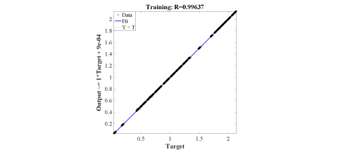
Figure 2. Convergence characteristics of FANN and ANN
(a) FANN
(b) ANN
Figure 3. Regression of the FANN and ANN
Figure 2 shows the convergence characteristics of the implementation of the FSA based optimum ANN (FANN) and the conventional ANN. The performance of the FANN and ANN are shown in Figure 3. The FANN has been achieved 0.99974; meanwhile the conventional ANN has been achieved 0.99637. This figure clearly shows the superiority of the FANN over the conventional ANN.
In this research, an improved neural network optimized with future search algorithm used to predict attenuation coefficient of 532 nm laser beam passing through an underwater channel in six of the Jerlov ocean water types (I, IB, II, III, 1C, 3C). The attenuation coefficient predicted for a different range of NaCl concentration and also the effect of air bubbles diameter, and air bubbles concentration are included in the total predict value of attenuation coefficient. Table 1 shows the minimal and maximum values of input parameters. These parameters have been carefully chosen to ensure that the training data are covering a wide range of oceans water variation scenarios.
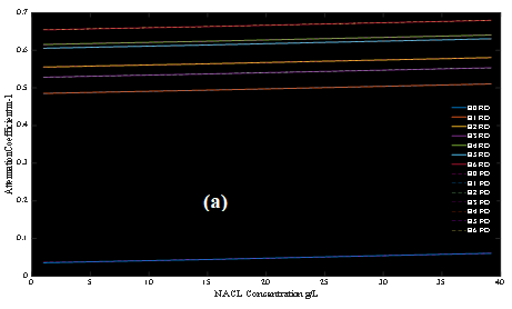
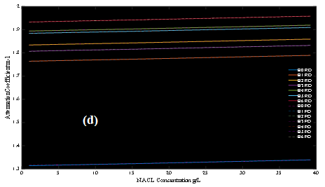
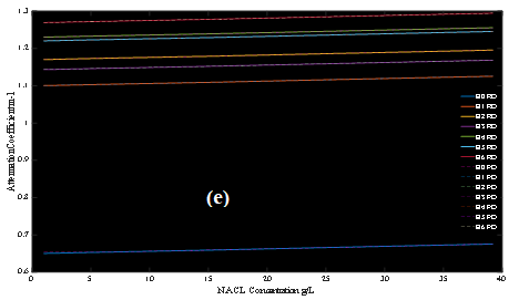
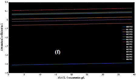
The Proposed FANN model was evaluated by comparing the predict values of the attenuation coefficient of 532 nm laser beam passing through an underwater channel obtained by the proposed model with the values of the attenuation coefficient of 532 nm laser beam passing through an underwater channel that measured practically as shown in Figure 4.
Figure 4 shows that the attenuation coefficient value predicted by FANN model is very close to the value measured practically. Moreover, FANN model shows an acceptable stable behavior in predicting the value of the attenuation coefficient when the value of NaCl concentration, air bubble diameter, and air bubbles concentration has been changed. Since the difference between attenuation coefficient value predicted by FANN model and the value measured practically is not clearly recognized in Figure 4, errors between predicted and practically measured attenuation coefficient were calculated and illustrated in Figure 5.
Table 1. Range of the covered training parameters
|
Training parameter |
Range |
|
Jerlov Water type |
I, IB, II, III, 1C, 3C |
|
NaCl concentration |
(0.5 – 40) g/L |
|
Air bubbles diameter |
0, 0.6 mm, 1.4 mm, 2.9 mm |
|
Air bubbles concentration |
0, 12 bubbles/cm3, 27 bubbles/cm3, 36 bubbles/cm3 |
(a) Jerlov type I(b) Jerlov type IB
(b) Jerlov type IB
(c) Jerlov type II
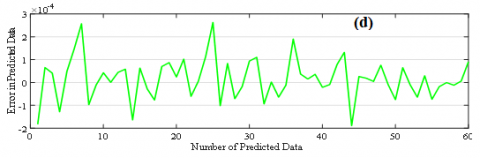
(d) Jerlov type III
(e) Jerlov type 1C(f) Jerlov type 3C
(f) Jerlov type 3C
Figure 4. Value of attenuation coefficient when measured practically and when predicted by proposed FANN model of the 532 nm laser beam passing through underwater channel for different concentration value of NaCl and different air bubbles concentration and diameter
(a) Jerlov type I
(b) Jerlov type IB
(c) Jerlov type II
(d) Jerlov type III
(e) Jerlov type 1C
(f) Jerlov type 3C
Figure 5. Errors in predicted values of attenuation coefficient obtained by proposed FANN
Figure 5 shows that the errors in the attenuation coefficient between its practically measured values and its predicted values by the proposed FANN model are very small. The errors are less than 10-4. Small errors values of the proposed FANN model indicate that this system is reliable and has an excellent performance in predicting the attenuation coefficient of 532 nm laser beam passing through an underwater channel. Although the errors show that the proposed FANN model has an excellent performance in estimating attenuation coefficient values.
For further evaluation, three standard error indices have been used to evaluate the performance of the proposed FANN model. These indices are mean square error (MSE), root mean square error (RMSE) and mean absolute error (MAE) as can be shown in Table 2.
Table 2. Error indices used to evaluate the performance of the proposed FANN model
|
Jerlov Water type |
MSE |
RMSE |
MAE |
|
I |
1.402 e-07 |
3.74E-04 |
1.12E-04 |
|
IB |
1.05E-07 |
3.25E-04 |
9.74E-05 |
|
II |
1.87E-07 |
4.32E-04 |
9.97E-05 |
|
III |
2.52E-07 |
5.02E-04 |
1.29E-04 |
|
1C |
4.05E-07 |
6.36E-04 |
1.27E-04 |
|
3C |
2.41E-07 |
4.91E-04 |
9.65E-05 |
The performance accuracy of the proposed FANN model inversely proportional to the standard error indices values, whenever MSE, RMSE, MAE values decrease indicates that the outputs of the proposed FANN model are more accurate. Table 2 shows that the proposed FANN model achieved an excellent performance and a reliable result in predicting the attenuation coefficient of 532 nm laser beam passing through an underwater channel.
The practical calculations processes of the attenuation coefficient for laser beam transmitted through underwater channel are a very challenging, costly and challenging procedure that actually requires precise observation and analysis to the numbers of parameters that specifically influence this calculation. Jerlov ocean water types, which defines numbers of optical parameters, NaCl concentration, air bubbles diameter, and air bubbles concentration are the key parameters which can affect the value of the attenuation coefficient. The FANN model is a new artificial intelligent method developed in this research to emulate transmission of 532nm laser beam in an underwater channel. The proposed FANN model predicts the attenuation coefficient of the 532nm laser beam. Errors in the values of the attenuation coefficient obtained by FANN model are lower than 10-4, where these values of errors are small and acceptable in evaluating proposed model performance. Three types of statistical analysis are used which are MSE, RMSE, and MAE. The maximum values of MSE, RMSE, and MAE showed that the proposed FANN model is exemplary and accurate in predicting the attenuation coefficient of the 532 nm laser beam in underwater optical channel. The proposed FANN model could therefore be used to determine an optical signal attenuation coefficient while moving through an underwater medium.
[1] Geldard, C.T., Thompson, J., Popoola, W.O. (2019). An overview of underwater optical wireless channel modelling techniques. 2019 International Symposium on Electronics and Smart Devices (ISESD), pp. 1-4. https://doi.org/10.1109/ISESD.2019.8909494
[2] Gussen, C.M., Diniz, P.S., Campos, M.L., Martins, W.A., Costa, F.M., Gois, J.N. (2016). A survey of underwater wireless communication technologies. J. Commun. Inf. Sys, 31(1): 242-255. https://doi.org/10.14209/jcis.2016.22
[3] Devito, L.M. (2008). Optical communication. Dig Tech Pap IEEE Int Solid-State Circuits Conf., 51: 218-218.
[4] Lacovara, P. (2008). High-bandwidth underwater communications. Marine Technology Society Journal, 42(1): 93-102. https://doi.org/10.4031/002533208786861326
[5] Giuliano, G. (2019). Underwater optical communication systems. Doctoral dissertation, University of Glasgow.
[6] Cossu, G., Sturniolo, A., Messa, A., Scaradozzi, D., Ciaramella, E. (2017). Full-fledged 10Base-T Ethernet underwater optical wireless communication system. IEEE Journal on Selected Areas in Communications, 36(1): 194-202. https://doi.org/10.1109/jsac.2017.2774702
[7] Jaddi, N.S., Abdullah, S., Hamdan, A.R. (2015). Optimization of neural network model using modified bat-inspired algorithm. Applied Soft Computing, 37: 71-86. https://doi.org/10.1016/j.asoc.2015.08.002
[8] Hemeida, A.M., Hassan, S.A., Mohamed, A.A.A., Alkhalaf, S., Mahmoud, M.M., Senjyu, T. (2020). Nature-inspired algorithms for feed-forward neural network classifiers: A survey of one decade of research. Ain Shams Engineering Journal, 11(3): 659-675. https://doi.org/10.1016/j.asej.2020.01.007
[9] Le, LT., Nguyen, H., Dou, J., Zhou, J. (2019). A comparative study of PSO-ANN, GA-ANN, ICA-ANN, and ABC-ANN in estimating the heating load of buildings’ energy efficiency for smart city planning. Applied Sciences, 9(13): 2630. https://doi.org/10.3390/app9132630
[10] Shareef, H., Ibrahim, A.A., Mutlag, A.H. (2015). Lightning search algorithm. Applied Soft Computing, 36: 315-333. https://doi.org/10.1016/j.asoc.2015. 07.028
[11] Mohammed Salim, O.N. (2017). New neuro-fuzzy system-based holey polymer fibers drawing process. AIP Advances, 7(10): 105301. https://doi.org/10.1063/1.4998270
[12] Chen, G., Zhu, M., Yu, H., Li, Y. (2007). Application of neural networks in image definition recognition. 2007 IEEE International Conference on Signal Processing and Communications, pp. 1207-1210. https://doi.org/10.1109/ICSPC.2007.4728542
[13] Nawi, N.M., Khan, A., Rehman, M.Z. (2013). A new back- propagation neural network optimized with cuckoo search algorithm. In: International Conference on Computational Science and Its Applications, pp. 413-426.
[14] Du, K.L. (2010). Clustering: A neural network approach. Neural Networks, 23(1): 89-107. https://doi.org/10.1016/j.neunet.2009.08.007
[15] Abualigah, L., Abd Elaziz, M., Hussien, A.G., Alsalibi, B., Jalali, S.M.J., Gandomi, A.H. (2020). Lightning search algorithm: A comprehensive survey. Applied Intelligence, 51: 2353-2376. https://doi.org/10.1007/s10489-020-01947-2AM
[16] Elsisi, M. (2019). Future search algorithm for optimization. Evolutionary Intelligence, 12(1): 21-31. https://doi.org/10.1007/s12065-018-0172-2
[17] Vrugt, J.A., Robinson, B.A., Hyman, J.M. (2008). Self-adaptive multimethod search for global optimization in real-parameter spaces. IEEE Transactions on Evolutionary Computation, 13(2): 243-259. https://doi.org/10.1109/tevc.2008.924428
[18] Anguita, D., Brizzolara, D., Parodi, G., Hu, Q., (2011). Optical wire- less underwater communication for AUV: Preliminary simulation and experimental results. OCEANS 2011 IEEE-Spain, 1-5. https://doi.org/10.1109/Oceans-Spain.2011.6003598
[19] Ali, M.F., Jayakody, D.N.K., Chursin, Y.A., Affes, S., Dmitry, S. (2020). Recent advances and future directions on underwater wireless communications. Archives of Computational Methods in Engineering, 27(5): 1379-1412. https://doi.org/10.1007/s11831-019- 09354-8
[20] Schirripa Spagnolo, G., Cozzella, L., Leccese, F. (2020). Underwater optical wireless communications: Overview. Sensors, 20(8): 2261. https://doi.org/10.3390/s20082261
[21] Chancey, M.A. (2005). Short range underwater optical communication links.
[22] Zeng, Z., Fu, S., Zhang, H., Dong, Y., Cheng, J. (2017). A survey of underwater optical wireless communications. IEEE Communications Surveys & Tutorials, 19(1): 204-238. https://doi.org/10.1109/comst. 2016.2618841
[23] Jerlov, N.G. (1977). Classification of sea water in terms of quanta irradiance. ICES Journal of Marine Science, 37(3): 281-287. https://doi.org/10.1093/icesjms/37.3.281
[24] Smith, R.C., Baker, K.S. (1978). Optical classification of natural waters 1. Limnology and Oceanography, 23(2): 260-267. https://doi.org/10.4319/lo.1978.23.2.0260
[25] Gregg, W.W., Rousseaux, C.S. (2017). Simulating PACE global ocean radiances. Frontiers in Marine Science, 4: 60. https://doi.org/10.3389/fmars.2017.00060
[26] Yang, X.S. (2014). Nature-Inspired Optimization Algorithms. Elsevier.
[27] Abiodun, O.I., Kiru, M.U., Jantan, A., Omolara A.E., Dada, K.V., Umar, A.M. (2019). Comprehensive review of artificial neural network applications to pattern recognition. IEEE Access, 7: 158820-158846. https://doi.org/10.1109/access.2019.2945545
[28] Palnitkar, R.M., Cannady, J. (2004). A review of adaptive neural networks. IEEE Southeast Conf., Proceedings, pp. 38-47. https://doi.org/10.1109/SECON.2004.1287896
[29] He, S., Wu, Q.H., Saunders, J.R. (2009). Group search optimizer: An optimization algorithm inspired by animal searching behavior. IEEE Transactions on Evolutionary Computation, 13(5): 973-990. https://doi.org/10.1109/tevc.2009.2011992
[30] Ramos, E.G., Martínez, F.V. (2013). A review of artificial neural networks: How well do they perform in forecasting time series? Analítika: Revista de Análisis Estadístico, (6): 7-18.
[31] Moayedi, H., Mosallanezhad, M., Rashid, A.S.A., Jusoh, W.A.W., Muazu, M.A. (2020). A systematic review and meta- analysis of artificial neural network application in geotechnical engineering: Theory and applications. Neural Computing and Applications, 32(2): 495-518. https://doi.org/10.1007/s00521-019- 04109-9