Syed Fazuruddin* | Seelam Sreekanth | G. Sankara Sekhar Raju
© 2021 IIETA. This article is published by IIETA and is licensed under the CC BY 4.0 license (http://creativecommons.org/licenses/by/4.0/).
OPEN ACCESS
Incompressible 2-D Navier-stokes equations for various values of Reynolds number with and without partial slip conditions are studied numerically. The Lid-Driven cavity (LDC) with uniform driven lid problem is employed with vorticity - Stream function (VSF) approach. The uniform mesh grid is used in finite difference approximation for solving the governing Navier-stokes equations and developed MATLAB code. The numerical method is validated with benchmark results. The present work is focused on the analysis of lid driven cavity flow of incompressible fluid with partial slip conditions (imposed on side walls of the cavity). The fluid flow patterns are studied with wide range of Reynolds number and slip parameters.
lid-driven cavity, square enclosure, partial slip conditions, finite difference scheme, Reynolds number
Worldwide for decades the numerical investigators in Computation Fluid Dynamics (CFD) have been left an indelible imprint to validate and justify their own developed numerical house-computational code with classical lid-driven cavity approach. From this approach research investigators have been increased the significance of numerical methods adopted for their essential outcomes. Lid driven square cavity problem is very interesting problem in computational fluid dynamics (CFD). Several numerical investigators have been investigating the fluid flow behavior within the top lid driven cavity for moderate Reynolds number (Re) values.
Several numerical methods are available in now a day to solve fluid flow problems like internal flows or external flows. The multi grid method was proposed by Ghia et al. [1], he employed a classical lid-driven flow problem for various Reynolds number as well as for different mesh sizes. As he produced a benchmark results which helped a lot to research investigator to correct their own developed computation numerical methods (or house – computational codes). Erturk et al. [2] presented a finite difference numerical approach with second order accuracy scheme on two-dimensional steady flow Navier-stoke equations for the Reynolds number Re≤ 21,000 with uniform mesh. Venkatadri et al. [3] proposed a numerical simulation of 2D incompressible driven cavity filled with Newtonian (K=0) and non-Newtonian fluid for various Reynolds numbers with uniform step along x and y-directions of computational domain. Gupta and Kalita [4] deliberated a different paradigm to solve 2D flow equation (Navier – Stokes) equations by incorporating bi-conjugate gradient model. They are examined fluid flow behavior within the enclosure (square and rectangular) by uniform translating upper lid for different Reynolds number. Adaptive grid mesh based Finite Volume paradigm is implemented on 2D flow equation (Navier – Stokes) by Magalhaes et al. [5]. They focused lid-driven cavity flow in 2D square geometry with Re=1000.
Vorticity – Stream function is a moderate technique to solve the Navier – Stoke equation. The stream function –vorticity formulation techniques is used widely by Erturk et al. [2, 6]. The fourth order compact finite difference scheme with ω-ψ technique is adopted Erturk et al. [6]. The Collocated Uniform grid system is used in ω-ψ technique and velocity – vorticity; it is very compactable to solve fluid flow problems. P – finite element-based stream function – vorticity approached numerical solution of lid – driven cavity problem is examined by Barragy and Carey [7] for the Reynolds number up to 12,500. The interesting study extracted from time derivative numerical solution of Navier – Stokes’s equations with primitive variable method for moderate Reynolds numbers has been proposed and explained in detailed through finite difference scheme by Erturk [8]. Obviously, ω-ψ technique is easy to apply one fluid flow problems and it gives more rigorous and effective results, due to its significance many researchers utilized this technique in their studies [9-11]. The staggered grid system is widely used in velocity – pressure method. The primitive variable velocity – pressure technique is imposed many fluid flow problems. Velocity – pressure method is validated with standard classical lid-driven cavity flow problem for many numerical investigators. Yapici et al. [12] examined lid-driven cavity problem by finite volume discretization is used in the developed computational code of semi-implicit method for pressure-linked equation (SIMPLE) algorithm for the Reynolds number Re=65,000. Wang et al. [13] aim to simulate the lid driven cavity flow problem for rage of Reynolds number Re=100-100000 by using semi-Lagrangian Vortex-In-Cell method.
The flow field examiners are conducted pioneer work past few decades on fluid flow characteristics inside the cavity with various numerical techniques by using appropriate numerical grid system [14-16]. Several numerical investigators have been investigating the fluid flow behavior within the top lid driven cavity for moderate Reynolds number (Re) values. Following the above studies, most of the authors neglected the influence of the momentum slip on lid driven cavity flow. The aim of the present problem is to study the fluid flow characteristics with the double lid driven cavity in the presence of partial slip conditions for different values of Reynolds number.
Consider 2-D regime with uniform sides (see in Figure 1). The governing partial differential equations of the interest of domain (square lid driven cavity) are the conservation of mass equation and momentum equations (Navier–Stokes’s equations). The fluid flow can be taken in this computation as incompressible and laminar. In these considerable assumptions the dimensional governing partial equations are as follows.
Figure 1. Schematic of problem
$\nabla .\overline{u}=0$ (1)
$\frac{\partial \overline{u}}{\partial t}+\left( \overline{u}.\nabla \right)\overline{u}\text{=}-\frac{1}{\rho }\nabla p+\upsilon {{\nabla }^{2}}\overline{u}$ (2)
Now introducing the stream function $\psi $ and vorticity $\overline{\omega }$ are dependent variables. The vorticity vector at a point is defined as twice the angular velocity and is:
$\overline{\omega }=\nabla \times \overline{u}$ (3)
Which is reduced in two dimensional flows in x-y plane is:
$\overline{\omega }\cdot \overline{k}=\frac{\partial v}{\partial x}-\frac{\partial u}{\partial y}$ (4)
For two-dimensional, incompressible flows, a scalar function may be defined in such a way that the equation of continuity is identically satisfied if the velocity components expressed in terms of such a function, are substituted in the continuity equation.
$\frac{\partial u}{\partial x}+\frac{\partial v}{\partial y}=0$ (5)
Such function is known as stream function, and is expressed by:
$\overline{u}=\nabla \times \psi \overline{k}$ (6)
The above expression in the Cartesian form is
$u=\frac{\partial \psi }{\partial y}\,\,\,\,\,\,\,\,\,\,\,\,\,v=-\frac{\partial \psi }{\partial x}$ (7)
The Poisson equation for the stream function ψ can be obtained from the equation $\overline{\omega }\cdot \overline{k}=\omega =\frac{\partial v}{\partial x}-\frac{\partial u}{\partial y}$ when the substituting of velocity components as stream function ψ. Thus, we have.
${{\nabla }^{2}}\psi =-\omega $ (8)
This is a kinematic equation connecting the ω and ψ. So, if we can find an equation for ω we will have obtained a formulation that automatically produces divergence-free velocity field. The vorticity transport equation is obtained from taking of curl of Eq. (2). Thus, we have,
$\frac{\partial \omega }{\partial t}+\mathbf{V}\cdot \nabla \omega =\upsilon {{\nabla }^{2}}\omega $ (9)
$R e=\frac{\rho U L}{\mu}$ is the Reynolds number ρ and μ are fluid density and viscosity respectively, U and L refers the Lid velocity and length of cavity respectively.
2.1 Slip and no-slip Conditions on Boundaries
The square enclosure bounded by four walls in which the horizontal walls are having no slip boundaries and the left and right sidewalls are move upward and a partial slip flow condition is imposed on these walls. It is considered that the partial slip in the left sidewall equals its corresponding value at the right one [i.e., Sl = Sr].
$t=0, u=v=0$ For $0 \leq y \leq 1 \quad 0 \leq X \leq 1$$\tau>0, u=v=0$ at $Y=0,1$ (10)
$u=0,\,\,\,\,\,V={{\lambda }_{l}}{{V}_{0}}+\chi \mu \frac{\partial v}{\partial x}$ at X=0 (11)
$u=0,\,\,\,\,\,V={{\lambda }_{r}}{{V}_{0}}+\chi \mu \frac{\partial v}{\partial x}$ at X=1 (12)
The following listed parameters are the non-dimensional variables.
$\begin{align} & \tau =\frac{t{{V}_{0}}}{{{L}^{2}}},\,\left( X,Y \right)=\frac{\left( x,y \right)}{L},U=\frac{u}{{{V}_{0}}}, \\ & V=\frac{v}{{{V}_{0}}}\,,\Psi =\frac{\psi }{L{{V}_{0}}},\Omega =\frac{\omega L}{{{V}_{0}}},{{S}_{l}}={{S}_{r}}=\frac{\chi \mu }{L} \\\end{align}$ (13)
The above mentioned non-dimensional variables are used in discussed boundary conditions are transformed in the vorticity stream function approach:
Along the left wall (X=0):
$u=0,\,\,\,\,\,\frac{\partial \Psi }{\partial X}={{\lambda }_{l}}+{{S}_{l}}\frac{{{\partial }^{2}}\Psi }{\partial {{X}^{2}}},\,\,\Omega =-\frac{{{\partial }^{2}}\Psi }{\partial {{X}^{2}}}$ (14)
Along the right wall (X=L):
$u=0,\,\,\,\,\,\frac{\partial \Psi }{\partial X}={{\lambda }_{r}}+{{S}_{r}}\frac{{{\partial }^{2}}\Psi }{\partial {{X}^{2}}},\,\,\Omega =-\frac{{{\partial }^{2}}\Psi }{\partial {{X}^{2}}}$ (15)
The non-dimensional governing equations of two-dimensional flow in a square enclosure with slip and without slip conditions
$\Omega =-\frac{{{\partial }^{2}}\Psi }{\partial {{X}^{2}}}-\frac{{{\partial }^{2}}\Psi }{\partial {{Y}^{2}}}$ (16)
$\frac{\partial \Omega }{\partial \tau }+U\frac{\partial \Omega }{\partial X}+V\frac{\partial \Omega }{\partial Y}=\frac{1}{\operatorname{Re}}{{\nabla }^{2}}\Omega $ (17)
The non-dimensional form of 2D axi-symmetric flows of Navier-Stokes’s equations in Vorticity () and Stream function () approach is given as
$\Omega =-\frac{{{\partial }^{2}}\Psi }{\partial {{X}^{2}}}-\frac{{{\partial }^{2}}\Psi }{\partial {{Y}^{2}}}$ (18)
$\frac{\partial \Omega }{\partial \tau }+U\frac{\partial \Omega }{\partial X}+V\frac{\partial \Omega }{\partial Y}=\frac{1}{\operatorname{Re}}{{\nabla }^{2}}\Omega $ (19)
The above-mentioned Eqns. (1) & (2), Re denotes the Reynolds number of the incompressible fluid flow, the velocity profiles along the X and Y directions are represents U and V respectively. By solving the above Eqns. (1) and (2) with pseudo time derivative and discretization explained in detailed as follows
$\Omega =-\frac{{{\partial }^{2}}\Psi }{\partial {{X}^{2}}}-\frac{{{\partial }^{2}}\Psi }{\partial {{Y}^{2}}}$ (20)
$\frac{\partial \Omega }{\partial \tau }=\frac{1}{\operatorname{Re}}{{\nabla }^{2}}\Omega -\frac{\partial \Psi }{\partial Y}\frac{\partial \Omega }{\partial X}+\frac{\partial \Psi }{\partial X}\frac{\partial \Omega }{\partial Y}$ (21)
The final solution will not be influenced by the order of pseudo time derivative in order to get the steady solution as we required. Therefore, an Explicit Euler Time step approach is implemented for these pseudo time derivatives to get first order $(\Delta t)$ accuracy approximation is used and the governing Eqns. (3) and (4) becomes
$\frac{{{\partial }^{2}}{{\Psi }^{n+1}}}{\partial {{X}^{2}}}-\frac{{{\partial }^{2}}{{\Psi }^{n+1}}}{\partial {{Y}^{2}}}={{\Omega }^{n}}$ (22)
$\begin{align} & {{\Omega }^{n+1}}-\Delta t\,\frac{1}{\operatorname{Re}}{{\nabla }^{2}}\Omega -\Delta t\frac{\partial {{\Psi }^{n}}}{\partial X}\frac{\partial {{\Omega }^{n+1}}}{\partial Y} \\ & \,\,\,+\Delta t\frac{\partial {{\Psi }^{n}}}{\partial Y}\frac{\partial {{\Omega }^{n+1}}}{\partial X}={{\Omega }^{n}} \\\end{align}$ (23)
The above equations in operator notation are as follows.
$\left( \frac{{{\partial }^{2}}}{\partial {{X}^{2}}}-\frac{{{\partial }^{2}}}{\partial {{Y}^{2}}} \right){{\Psi }^{n+1}}={{\Omega }^{n}}$ (24)
$\left( \begin{align} & 1-\Delta t\,\frac{1}{\operatorname{Re}}\left( \frac{{{\partial }^{2}}}{\partial {{X}^{2}}}+\frac{{{\partial }^{2}}}{\partial {{Y}^{2}}} \right) \\ & -\Delta t{{\left( \frac{\partial \Psi }{\partial X} \right)}^{n}}\frac{\partial }{\partial Y} \\ & +\Delta t{{\left( \frac{\partial \Psi }{\partial Y} \right)}^{n}}\frac{\partial }{\partial X} \\\end{align} \right){{\Omega }^{n}}={{\Omega }^{n+1}}$ (25)
In the numerical solution of Eqns. (7) & (9) are strictly used second order discretization’s (see in Table 1) and also consider the uniform mesh length.
Table 1. Second order central discretization
|
${{\chi }_{x}}$ |
$\,\frac{{{\chi }_{i+1,j}}-{{\chi }_{i-1,j}}\,}{2\Delta x}\,\,$ |
|
${{\chi }_{y}}\,$ |
$\frac{{{\chi }_{i,j+1}}-{{\chi }_{i,j-1}}\,}{2\Delta y}$ |
|
${{\chi }_{xx}}$ |
$\frac{{{\chi }_{i+1,j}}-2{{\chi }_{i,j}}\,+{{\chi }_{i-1,j}}}{\Delta {{x}^{2}}}$ |
|
${{\chi }_{yy}}$ |
$\frac{{{\chi }_{i,j+1}}-2{{\chi }_{i,j}}\,+{{\chi }_{i,j-1}}}{\Delta {{y}^{2}}}$ |
|
${{\chi }_{xy}}$ |
$\frac{{{\chi }_{i+1,j+1}}-{{\chi }_{i-1,j+1}}-{{\chi }_{i+1,j-1}}+{{\chi }_{i-1,j-1}}}{2\Delta x\Delta y}$ |
The developed house computational MATLAB code is performed in the present problem and obtained fluid flow patterns with the following convergence criteria.
$\left( 1-\frac{{{\partial }^{2}}}{\partial {{X}^{2}}} \right)\left( 1-\frac{{{\partial }^{2}}}{\partial {{Y}^{2}}} \right){{\Psi }^{n+1}}={{\Psi }^{n}}+{{\Omega }^{n}}$ (26)
$\begin{align} & \left( 1-\Delta t\,\frac{1}{\operatorname{Re}}\frac{{{\partial }^{2}}}{\partial {{X}^{2}}}+\Delta t{{\left( \frac{\partial \Psi }{\partial Y} \right)}^{n}}\frac{\partial }{\partial X} \right) \\ & \left( 1-\Delta t\,\frac{1}{\operatorname{Re}}\frac{{{\partial }^{2}}}{\partial {{Y}^{2}}}-\Delta t{{\left( \frac{\partial \Psi }{\partial X} \right)}^{n}}\frac{\partial }{\partial Y} \right){{\Omega }^{n+1}}={{\Omega }^{n}} \\\end{align}$ (27)
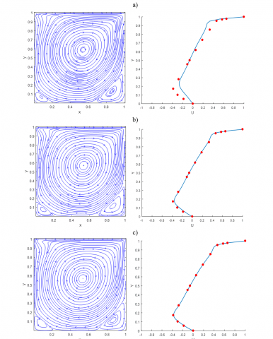
Results (seen in Figure 2) obtained through the methods of Vorticity-Stream function formulation (VSF) shows an excellent agreement with [1] for Re=1000. This comparison test gives the confidence on developed house-computational MATLAB Code for the further investigations.
Figure 2. Finite difference simulation of Streamlines and centerline velocity profile for various mesh sizes at Re=1000. a) Grid size 41X41, b) Grid size 81X81 and c) Grid size 129X129. Solid line -Present work (FDM-VSF) and red dots – Ghia et al. [1]
This section illustrates the fluid flow patterns with driven cavity for various values of Reynolds numbers with the impact of velocity slip influences, the fluid flow patterns for wide range of controlling key parameters such as Re = 50-1000, Sl=Sr=S=0.2-1.0 and with fixed lid driven control parameters λl=1, λr=-1. The implemented numerical method is validated with Ghia et al. [1], the detailed validation is presented in Figure 2, the streamline patterns at Re=1000 along with central line velocity are obtained for different grid sizes (i.e. 41X41, 81X81 and 129X129). The vertical central line velocity profile mapped with Ghia et al. [1] which gives an excellent agreement for the grid size 81X81 and 129X129.This comparison test gives the confidence for further computations with grid size 81X81. It is worth noting that side walls driven uniformly with the values of control parameters λl=1, λr=-1. Figure 3 represents the simulation of streamline pattern at Re=100 with velocity partial slip-onside walls S=1, here uniform horizontal streamline patterns are generated and the respective central line velocity profiles are also visualized. The minor vortices are formed near the side walls, which are generated by the walls, are driven in opposite directions. In Figure 4, when Re=400 the uniform streamline vortex pattern upsurge and the shape of the vortex is slightly shifted from horizontal position to diagonal position with minor vortices. In Figure 5, Rising the Reynolds number Re=1000 the vortex pattern is fully upraised form horizontal to diagonal mode and also the minor cells are merged, the shape of the vortex is changed from dumbbell to oval which shows that the fluid flow rises with the increase of Re values in presence of partial slip-on right wall.
Mid-section velocity profile of U for Re=1000 by varying the slip parameter S from 0.2 to 1.0 is depicted in Figure 6. This depicted plot explains, when velocity slip parameter rises from 0.2 to 1.0 it is observed that the flow pattern is uniformly twisted once at Y=0.5 and also the velocity of the fluid decreases when the right driven wall in positive (λl=1) direction and left wall driven in negative (λr=-1) direction. The Figure 7 shows mid-section V velocity profile for Re=1000 with the variation of Slip parameter S from 0.2 to 1.0. The presented plot expressed when slip parameter rises from 0.2 to 1.0 it is observed that the flow pattern is uniformly symmetric at X = 0.5. The velocity of the fluid upsurge near the right driven wall in positive (λl=1) direction and rise down the flow on left driven wall in negative (λl=-1) direction. The fluid flow velocity is gradually reducing when increasing of velocity slip parameter S.
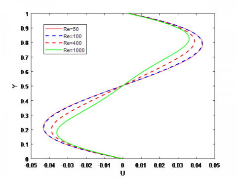
The variation on fluid velocity (velocity profile U with vertical direction) with the various values of Reynolds numbers Re and λl=1, λr=-1, Sl=Sr=S=1 is shown in Figure 8. This figure deliberates that as the Reynolds number Re increases from 50 to 1000 the flow pattern is uniformly symmetric at Y=0.5 and the U velocity is diminishes. That is the respective fluid flow velocity inside the cavity up rises at left driven wall and rises down near right driven wall of the enclosure and the fluid flow occupies the entire cavity.
Figure 3. Finite difference simulation of Streamlines – (a) and centerline velocity profiles – (b&c) for λl=1, Sl=1, Re=100, λr=-1, Sr=1
Figure 4. Finite difference simulation of Streamlines and centerline velocity profiles for λl=1, Sl=1, Re=400, λr=-1, Sr=1
Figure 5. Finite difference simulation of Streamlines and centerline velocity profiles for λl=1, Sl=1, Re=1000, λr=-1, Sr=1
Figure 6. Mid-section velocity profile of U for Re=1000 and λl=1, λr=-1, Sl=Sr=S
Figure 7. Mid-section velocity profile of V for Re=1000 and λl=1, λr=-1, Sl=Sr=S
Figure 8. Mid-section velocity profile of U for λl=1, λr=-1, Sl=Sr=S
The variation on fluid velocity (velocity profile V with horizontal direction) with the various values of Reynolds numbers Re and λl=1, λr=-1, Sl=Sr=S=1 is shown in Figure 9. It is expressed that as the Reynolds number Re increases from 50 to 1000 the flow pattern is uniformly symmetric at X=0.5 and the V velocity is raise down. That is the respective fluid flow velocity inside the cavity up rises at left driven wall and rises down near right driven wall of the enclosure.
Figure 9. Mid-section velocity profile of U for λl=1, λr=-1, Sl=Sr=S
The two-dimensional laminar incompressible double lid (λl=1, λr=-1) driven cavity flow under the effects of velocity slip conditions and Vorticity stream function approach has been examined numerically. Lid driven square cavity problem is a very interesting problem in computational fluid dynamics (CFD). Several numerical investigators have been investigating the fluid flow behavior within the top lid driven cavity for moderate Reynolds number (Re) values. Most of the lid driven cavity problems having only no-slip boundary conditions while in this investigation we considered slip and no-slip boundary conditions for various values of Re. The governing Partial differential equations with slip and no slip boundary conditions have been employed by finite difference method. Investigation of the control parameters influence on flow structures within the enclosure has been performed. It has been found that velocity slip parameter can be a good control parameter which allows changing the fluid flow velocity profiles regardless of Reynolds number values. Gradual reduction of fluid velocity is noticed for the incremental values in velocity slip parameter S. When the Reynolds number Re varies from 50 to 1000 a uniformly symmetric flow patterns are observed about the lines X= 0.5 and Y=0.5 respectively. The future works focused on natural convective internal flows with slip influence and manage the heat transport performance by controlling the fluid flow velocity.
|
L |
Length scale |
|
P |
Dimensionless pressure |
|
Re |
Reynolds number |
|
Sl |
Partial slip in the left sidewall |
|
Sr |
Partial slip in the Right sidewall |
|
t |
Time |
|
U |
Lid velocity |
|
u, v |
Dimensionless velocity components in X and Y direction respectively |
|
V0 |
Side walls velocity |
|
Greek symbols |
|
|
$\psi$ |
Non-dimensional stream function |
|
λl |
Left Wall driven control parameter |
|
λr |
Right Wall driven control parameter |
|
ω |
Non-dimensional vorticity function |
|
$\nabla$ |
Laplacian operator |
|
$\rho$ |
Fluid density of the particles |
|
v |
Kinematic viscosity |
|
$\mu$ |
Dynamic viscosity |
|
Ω |
Vorticity function |
|
τ |
Non-dimensional time function |
|
Ψ |
Stream function |
|
Subscripts |
|
|
l |
Left |
|
r |
Right |
|
0 |
Initial value |
[1] Ghia, U., Ghia, K.N., Shin, C.T. (1982). High-Re solutions for incompressible flow using the Navier Stokes equations and a multigrid method. Journal of Computational Physics, 48(3): 387-411. https://doi.org/10.1016/0021-9991(82)90058-4
[2] Erturk, E., Corke, T.C., GoKcol, C. (2005). Numerical solutions of 2-D steady incompressible driven cavity flow at high Reynolds numbers. Int. J. Numer. Meth. Fluids, 48(7): 747-774. https://doi.org/10.1002/fld.953
[3] Venkatadri, K., Maheswari, S., Venkata Lakshmi, C., Ramachandra Prasad, V. (2018). Numerical simulation of lid-driven cavity flow of micropolar fluid. IOP Conf. Series: Materials Science and Engineering, 402(1): 012168. https://doi.org/10.1088/1757-899X/402/1/012168
[4] Gupta, M.M., Kalita, J.C. (2005). A new Paradigm for solving Navier-Stokes’s equations: Stream function – Velocity formulation. Journal of computational Physics, 207(1): 52-68. https://doi.org/10.1016/j.jcp.2005.01.002
[5] Magalhaes, J.P.P., Albuquerque, D.M.S., Pereira, J.M.C., Pereira, J.C.F. (2013). Adaptive mesh Finite Volume calculation of 2D lid cavity corner vortices. Journal of Computational Physics, 243: 365-381. https://doi.org/10.1016/j.jcp.2013.02.042
[6] Erturk, E., GoKcol, C. (2006). Fourth-order Compact formulation Navier – Stokes equations and driven cavity flow at high Reynolds numbers. International journal for Numerical Methods in Fluids, 50(4): 421-436. https://doi.org/10.1002/fld.1061
[7] Barragy, E., Carey, G.F. (1997). Stream function – Vorticity driven cavity solution using p finite elements. Computers & Fluids, 26(5): 453-468. https://doi.org/10.1016/S0045-7930(97)00004-2
[8] Erturk, E. (2009). Comparison of wide and compact Fourth – order formulation of Navier – Stokes’s equations. International journal for Numerical Methods in Fluids, 60(9): 992-1010. https://doi.org/10.1002/fld.1920
[9] Venkatadri, K., Anwar Beg, O., Rajarajeswari, P., Ramachandra Prasad, V. (2020). Numerical simulation of thermal radiation influence on natural convection in a trapezoidal enclosure: Heat flow visualization through energy flux vectors. International Journal of Mechanical Sciences, 171: 105391. https://doi.org/10.1016/j.ijmecsci.2019.105391
[10] Venkatadri, K., Abdul Gaffar, S., Suryanarayana Reddy, M., Ramachandra Prasad, V., Hidayathulla Khan, B.M., Anwar Beg, O. (2020). Melting heat transfer on Magnetohydrodynamics buoyancy convection in an enclosure: A numerical study. Journal of Applied and Computational Mechanics 6(1): 52-62. https://doi.org/10.22055/JACM.2019.28761.1504
[11] Venkatadri, K., Abdul Gaffar, S., Ramachandra Prasad, V., Hidayathulla Khan, B.M., Anwar Beg, O. (2019). Simulation of natural convection heat transfer in a 2-D trapezoidal enclosure. International Journal of Automotive and Mechanical Engineering, 16(4): 7375-7390. https://doi.org/10.15282/ijame.16.4.2019.13.0547
[12] Yapici, K., Uludag, Y. (2013). Finite Volume simulation of 2-D steady square lid driven cavity flow at high Reynolds number. Brazilian journal of Chemical Engineering, 30(4): 923-937. https://doi.org/10.1590/S0104-66322013000400023
[13] Wang, C., Sun, J.J, Ba, Y. (2017). A semi-Lagrangian Vortex-In-Cell method and its application to high-Re lid-driven cavity flow. International Journal of Numerical Methods for Heat & Fluid Flow, 27(6): 1186-1214. https://doi.org/10.1108/HFF-08-2015-0320
[14] Venkatadri, K., GouseMohiddin, S., Suryanarayana Reddy, M. (2017). Hydromagneto quadratic natural convection on a lid driven square cavity with isothermal and non-isothermal bottom wall. Engineering Computations, 34(8): 2463-2478. https://doi.org/10.1108/EC-06-2017-0204
[15] Venkatadri, K., GouseMohiddin, S., Suryanarayana Reddy, M. (2017). Mathematical modelling of unsteady MHD double diffusive natural convection flow in a square cavity. Frontiers in Heat and Mass Transfer, 9: 33. http://dx.doi.org/10.5098/hmt.9.33
[16] Hidayathulla Khan, B.M., Venkatadri, K., Anwar Be´g, O., Ramachandra Prasad, V., Mallikarjuna, B. (2018). Natural convection in a square cavity with uniformly heated and/or insulated walls using marker-and-cell method. International Journal of Applied and Computational Mathematics, 4: 61. https://doi.org/10.1007/s40819-018-0492-z