Charles C. Ike
© 2021 IIETA. This article is published by IIETA and is licensed under the CC BY 4.0 license (http://creativecommons.org/licenses/by/4.0/).
OPEN ACCESS
The Fourier integral method was used in this work to determine the stress fields in a two dimensional (2D) elastic soil mass of semi-infinite extent subject to line and strip loads of uniform intensity acting on the boundary. The two dimensional plane strain problem was formulated using stress-based method. The Fourier integral was used to transform the biharmonic stress compatibility equation to a fourth order linear ordinary differential equation (ODE) in terms of the stress function. The ODE was solved subject to the boundedness condition to obtain the bounded stress function. Cartesian stress components were obtained using the Love stress functions. Application of the stress boundary conditions for the case of line load of uniform intensity and the cases of uniformly distributed load on a strip of finite width gave the respective unknown constants of the Love stress functions; and hence the complete determination of the Cartesian stress components for the two cases considered. Inversion of the Fourier integral expressions obtained for the normal and shear stresses in the Fourier parameter gave respective expressions for the normal and shear stress fields for line and finite strip loads of finite width in the physical domain variables. The results obtained agreed with the results from previous studies which used displacement based methods.
Fourier integral method, two dimensional elasticity problem in plane strain, Love stress function, biharmonic stress compatibility equation
The analysis and design of road pavements, bridge structures, building foundations, retaining walls, piles, piers and water reservoirs entail analysis of the stress, strain and deformation in the supporting soil as a result of the applied external loads. This is because the structures are founded on soil which is required to withstand the resulting stresses and deformations without the occurrence of failures of the soil [1-4]. The problems of the determination of stresses, strains and displacement fields in masses of soil idealised as semi-infinite in extent, and assumed to be linearly elastic are problems of the classical mathematical theory of elasticity [1, 5-10]. They are called elastic half-space problems if the soil mass is modelled as semi-infinite and occupying the half-space region defined in Cartesian coordinates as -∞≤x≤∞; -∞≤y≤∞; 0≤z≤∞.
Otherwise, when the soil mass occupies a two dimensional region of space which is of semi-infinite extent, the problems become elastic half-plane problems [11-13]. Problems of the mathematical theory of elasticity are formulated using the differential equations of equilibrium, the generalised Hooke’s stress – strain laws and the geometric (kinematic) relations together with the deformation and traction boundary conditions [5-13]. The governing equations for such problems are usually complicated when heterogeneity and anisotropy are considered. They are also complicated by considerations of non-linearities in the stress – strain behaviours. Even for considerations of homogenous, isotropic and linearly elastic materials, the governing equations for three dimensional cases are a system of fifteen equations in terms of fifteen unknown variables, namely six Cauchy stress components, three Cartesian displacement components, and six strain components. For two dimensional elasticity problems, the number of governing equations is reduced but the solution for the unknowns is still rendered difficult by the relatively high number of governing equations.
Research efforts to solve elasticity problems in three and two dimensions have led to the formulation and development of three methods, namely: stress-based methods, displacement based methods and mixed (hybrid) methods. Stress-based methods for formulation of elasticity problems entail the simultaneous formulation of the governing equations involving the differential equations of equilibrium, the stress – strain relations and the kinematic relations such that the stresses are the primary unknown variables. This achieves a reduction in the number of governing equations from fifteen to six for three dimensional problems [5-13]. Similarly, the displacement based method involve a reformulation of the governing equations to have the three displacement components as the primary unknowns. The merit of the displacement based method is the reduction in the number of governing equations to be solved from fifteen to three for three dimensional problems, and to two for two dimensional problems. The mixed or hybrid methods which are not common, involve the reformulation of the governing equations to have the primary unknowns as some stress components and some displacement components. All the three methods involve a simplification of the governing equations due to the reduction in the number of equations to be solved. Displacement based methods were developed by Navier, Lamé, Boussinesq, Papkovich, Neuber, Green and Zerna. Stress based methods were developed by Airy, Beltrami, Michell, Love and Morera.
The advantages and merits offered by the displacement and stress-based methods have led researchers to develop solutions to the governing equations of the displacement and stress-based methods. Such solutions, which satisfy the governing equations of the displacement and stress-based methods are called respectively displacement functions and stress functions [14-32]. Some displacement functions of the theory of elasticity are: Green and Zerna potential (harmonic) displacement function, Boussinesq displacement functions. Some stress functions of the theory of elasticity are: Airy’s stress function, Love stress function and Green and Zerna stress potential function.
Ike [12] used the exponential Fourier transform method to solve the theory of elasticity problem of finding Cartesian stresses in elastic half-plane soils due to load applied on the boundary. Onah et al. [18] used the Fourier transform method to determine Cartesian stress components caused by infinitely long line loads on semi-infinite elastic soils. Onah et al. [8] used the Fourier transform method to determine the Cartesian stress field components in semi-infinite, linear elastic soil in the xz coordinate plane due to infinitely long line load and uniformly distributed load applied on a finite strip -a≤x≤a on the boundary.
The main goal of this research is to use the Fourier integral method for solving two dimensional elasticity problems in plane strain. The specific objectives include:
(i) to present the two dimensional elasticity problem in plane strain conditions using a stress-based formulation.
(ii) to apply the Fourier integral transformation to the biharmonic stress compatibility equation of the stress-based formulation, and obtain a simplification of the boundary value problem to a fourth order ordinary differential equation (ODE) in the Fourier integral space.
(iii) to solve the resulting fourth order ODE to obtain bounded solution for the stress functions for the half-plane.
(iv) to use Love stress functions and obtain the Cauchy’s stresses in the Fourier integral space.
(v) to enforce boundary conditions for line and strip loads and obtain the integration constants.
(vi) to apply Fourier integral inversion formulae and obtain the stresses in the physical domain variables.
2.1 Field equations of 2D elasticity
The field equations for plane strain elasticity are: the strain – displacement relations [11-13], the stress-strain equations, and the differential equations of equilibrium. The strain-displacement relations are given by:
${{\varepsilon }_{xx}}=\frac{\partial u}{\partial x}$ (1)
${{\varepsilon }_{zz}}=\frac{\partial w}{\partial z}$ (2)
${{\varepsilon }_{xz}}=\frac{1}{2}\left( \frac{\partial u}{\partial z}+\frac{\partial w}{\partial x} \right)$ (3)
${{\varepsilon }_{xy}}={{\varepsilon }_{yz}}={{\varepsilon }_{yy}}=0$ (4)
where, $\mathcal{E}_{x x}, \quad \mathcal{E}_{y y,} \quad \mathcal{E}_{z z}$ are normal strains, $\varepsilon_{x z}, \varepsilon_{x y,} \varepsilon_{y z}$ are shear strains and u, w are displacement components in the x, and z Cartesian coordinate directions.
Saint Venant’s strain compatibility equation is [11-13]:
$\frac{{{\partial }^{2}}{{\varepsilon }_{xx}}}{\partial {{z}^{2}}}+\frac{{{\partial }^{2}}{{\varepsilon }_{zz}}}{\partial {{x}^{2}}}=2\frac{{{\partial }^{2}}{{\varepsilon }_{xz}}}{\partial x\partial z}$ (5)
The stress – strain relations (equations) are [11-13]:
${{\sigma }_{xx}}=(\lambda +2G){{\varepsilon }_{xx}}+\lambda {{\varepsilon }_{zz}}$ (6)
${{\sigma }_{zz}}=(\lambda +2G){{\varepsilon }_{zz}}+\lambda {{\varepsilon }_{xx}}$ (7)
${{\sigma }_{yy}}=\lambda {{\varepsilon }_{xx}}+\lambda {{\varepsilon }_{zz}}$ (8)
${{\tau }_{xz}}={{\sigma }_{xz}}=2G{{\varepsilon }_{xz}}=G{{\gamma }_{xz}}$ (9)
${{\tau }_{xy}}={{\tau }_{yz}}=0$ (10)
where, $\sigma_{x x}, \sigma_{y y} \sigma_{z z}$ are normal stresses; $\tau_{x z}\left(\sigma_{x z}\right), \tau_{x y}, \tau_{y z}$ are shear stresses; G is the shear modulus and l is the Lamé’s constant. The differential equations of equilibrium are given by:
$\frac{\partial {{\sigma }_{xx}}}{\partial x}+\frac{\partial {{\tau }_{xz}}}{\partial z}+{{f}_{x}}=0$ (11)
$\frac{\partial {{\tau }_{xz}}}{\partial x}+\frac{\partial {{\sigma }_{zz}}}{\partial z}+{{f}_{z}}=0$ (12)
where, fx and fz are body forces.
For plane strain, the Navier’s displacement equilibrium equations are given by the system of two partial differential equations in terms of the two displacement components [19]:
$G{{\nabla }^{2}}u+(\lambda +G)\frac{\partial }{\partial x}\left( \frac{\partial u}{\partial x}+\frac{\partial w}{\partial z} \right)+{{f}_{x}}=0$ (13)
$G{{\nabla }^{2}}w+(\lambda +G)\frac{\partial }{\partial z}\left( \frac{\partial u}{\partial x}+\frac{\partial w}{\partial z} \right)+{{f}_{z}}=0$ (14)
${{\nabla }^{2}}=\frac{{{\partial }^{2}}}{\partial {{x}^{2}}}+\frac{{{\partial }^{2}}}{\partial {{z}^{2}}}$ (15)
where, $\nabla^{2}$ is the Laplace differential operator.
Alternative forms of Navier’s displacement formulation of plane strain elasticity problems are:
$G{{\nabla }^{2}}u+\frac{E}{2(1+\mu )(1-2\mu )}\frac{\partial }{\partial x}\left( \frac{\partial u}{\partial x}+\frac{\partial w}{\partial z} \right)+{{f}_{x}}=$$G{{\nabla }^{2}}u+\frac{G}{(1-2\mu )}\frac{\partial }{\partial x}\left( \frac{\partial u}{\partial x}+\frac{\partial w}{\partial z} \right)+{{f}_{x}}=0$ (16)
$G{{\nabla }^{2}}w+\frac{E}{2(1+\mu )(1-2\mu )}\frac{\partial }{\partial z}\left( \frac{\partial u}{\partial x}+\frac{\partial w}{\partial z} \right)+{{f}_{z}}=$$G{{\nabla }^{2}}w+\frac{G}{(1-2\mu )}\frac{\partial }{\partial z}\left( \frac{\partial u}{\partial x}+\frac{\partial w}{\partial z} \right)+{{f}_{z}}=0$ (17)
where, E denotes the modulus of elasticity and $\mu$ is the Poisson’s ratio.
Navier’s equation for the displacement formulation of plane stress problems are [19]:
$G{{\nabla }^{2}}u+\frac{E}{2(1-\mu )}\frac{\partial }{\partial x}\left( \frac{\partial u}{\partial x}+\frac{\partial w}{\partial z} \right)+{{f}_{x}}=0$ (18)
$G{{\nabla }^{2}}w+\frac{E}{2(1-\mu )}\frac{\partial }{\partial z}\left( \frac{\partial u}{\partial x}+\frac{\partial w}{\partial z} \right)+{{f}_{z}}=0$ (19)
where for plane stress elasticity, the boundary conditions are $\gamma_{y z}=\gamma_{x z}=0$.
The surface tractions (stress boundary conditions) are:
$\left( \begin{matrix} {{t}_{x}} \\ {{t}_{z}} \\\end{matrix} \right)=\left( \begin{matrix} {{\sigma }_{xx}} & {{\sigma }_{xz}} \\ {{\sigma }_{xz}} & {{\sigma }_{zz}} \\\end{matrix} \right)\left( \begin{matrix} {{n}_{x}} \\ {{n}_{z}} \\\end{matrix} \right)$ (20)
where, tx, tz are tractions, and nx, nz are direction cosines.
For plane stress, the field equations are:
Stress – strain relations:
${{\varepsilon }_{xx}}=\frac{1}{E}({{\sigma }_{xx}}-\mu {{\sigma }_{zz}})$ (21)
${{\varepsilon }_{zz}}=\frac{1}{E}({{\sigma }_{zz}}-\mu {{\sigma }_{xx}})$ (22)
${{\varepsilon }_{yy}}=\frac{1}{E}(-\mu {{\sigma }_{xx}}-\mu {{\sigma }_{zz}})=-\frac{\mu }{E}({{\sigma }_{xx}}+{{\sigma }_{zz}})$ (23)
${{\varepsilon }_{xz}}=\frac{(1+\mu )}{E}{{\sigma }_{xz}}=\frac{{{\sigma }_{xz}}}{2G}$ (24)
${{\varepsilon }_{yy}}=\frac{-\mu }{1-\mu }({{\varepsilon }_{xx}}+{{\varepsilon }_{zz}})$ (25)
Strain – displacement equations:
$\left( \begin{matrix} {{\varepsilon }_{xx}} \\ {{\varepsilon }_{yy}} \\ {{\varepsilon }_{zz}} \\ 2{{\varepsilon }_{xz}} \\\end{matrix} \right)=\left( \begin{matrix} \frac{\partial }{\partial x} & 0 & 0 \\ 0 & \frac{\partial }{\partial y} & 0 \\ 0 & \frac{\partial }{\partial z} & 0 \\ \frac{\partial }{\partial z} & 0 & \frac{\partial }{\partial x} \\\end{matrix} \right)\left( \begin{matrix} u \\ v \\ w \\\end{matrix} \right)$ (26)
where, $\varepsilon_{y z}=\varepsilon_{x y}=0$.
Saint Venant’s compatibility equations for plane stress is still given by Eq. (5).
The differential equations of equilibrium for plane stress conditions are identical with those of plane strain. The field equations become for plane stress, Navier’s displacement equilibrium equation [19] given in Eqns. (18) and (19).
2.2 Airy’s stress function formulation
The Beltrami – Michell stress compatibility equations are written in general as [32]:
${{\nabla }^{2}}({{\sigma }_{xx}}+{{\sigma }_{zz}})=C(\mu )\left( \frac{\partial {{f}_{x}}}{\partial x}+\frac{\partial {{f}_{z}}}{\partial z} \right)$ (27)
where,
$C(\mu )=-(1+\mu )$ (28)
for plane stress and,
$C(\mu )=\frac{-1}{1-\mu }$ (29)
for plane strain.
Airy solved the 2D elasticity problems by defining stress potential functions φ(x,z) that satisfy the differential equations of equilibrium as follows:
${{\sigma }_{xx}}=\frac{{{\partial }^{2}}\varphi }{\partial {{z}^{2}}}+V$ (30)
${{\sigma }_{zz}}=\frac{{{\partial }^{2}}\varphi }{\partial {{x}^{2}}}+V$ (31)
${{\tau }_{xz}}=-\frac{{{\partial }^{2}}\varphi }{\partial x\partial z}$ (32)
where, V is the potential function for the body forces fx and fz and can be given by:
${{f}_{x}}=-\frac{\partial V}{\partial x}$ (33)
${{f}_{z}}=-\frac{\partial V}{\partial z}$ (34)
where,
$\frac{\partial {{f}_{x}}}{\partial z}=\frac{\partial {{f}_{z}}}{\partial x}$ (35)
Note:
$\frac{\partial }{\partial x}\left( \frac{{{\partial }^{2}}\varphi }{\partial {{z}^{2}}}+V \right)+\frac{\partial }{\partial z}\left( -\frac{{{\partial }^{2}}\varphi }{\partial x\partial z} \right)+{{f}_{x}}=0$ (36)
\(\frac{{{\partial }^{3}}\varphi }{\partial x\partial {{z}^{2}}}+\frac{\partial V}{\partial x}-\frac{{{\partial }^{3}}\varphi }{\partial x\partial {{z}^{2}}}+{{f}_{x}}=0\) (37)
which is true since $f_{x}=-\frac{\partial V}{\partial x}$.
$\frac{\partial }{\partial z}\left( \frac{{{\partial }^{2}}\varphi }{\partial {{x}^{2}}}+V \right)-\frac{\partial }{\partial x}\left( \frac{{{\partial }^{2}}\varphi }{\partial x\partial z} \right)+{{f}_{z}}=0$ (38)
$\frac{{{\partial }^{3}}\varphi }{\partial z\partial {{x}^{2}}}+\frac{\partial V}{\partial z}-\frac{{{\partial }^{3}}\varphi }{\partial {{x}^{2}}\partial z}+{{f}_{z}}=0$ (39)
which is true since $f_{z}=-\frac{\partial V}{\partial z}$.
Then, the Beltrami – Michell stress compatibility equation becomes:
\({{\nabla }^{2}}\left( \frac{{{\partial }^{2}}\varphi }{\partial {{z}^{2}}}+V+\frac{{{\partial }^{2}}\varphi }{\partial {{x}^{2}}}+V \right)=C(\mu )\left( \frac{\partial {{f}_{x}}}{\partial x}+\frac{\partial {{f}_{z}}}{\partial z} \right)\) (40)
\({{\nabla }^{2}}\left( \frac{{{\partial }^{2}}\varphi }{\partial {{x}^{2}}}+\frac{{{\partial }^{2}}\varphi }{\partial {{z}^{2}}} \right)+2{{\nabla }^{2}}V=C(\mu )\left( \frac{\partial {{f}_{x}}}{\partial x}+\frac{\partial {{f}_{z}}}{\partial z} \right)\) (41)
${{\nabla }^{2}}{{\nabla }^{2}}\varphi (x,z)+2{{\nabla }^{2}}V=C(\mu )\left( \frac{\partial {{f}_{x}}}{\partial x}+\frac{\partial {{f}_{z}}}{\partial z} \right)$ (42)
When body forces are absent, the Beltrami – Michell stress compatibility equation simplifies to the biharmonic equation in terms of the Airy’s stress potential function:
${{\nabla }^{2}}{{\nabla }^{2}}\varphi (x,z)={{\nabla }^{4}}\varphi (x,z)=0$ (43)
where,
${{\nabla }^{4}}={{\nabla }^{2}}{{\nabla }^{2}}$$=\left( \frac{{{\partial }^{4}}}{\partial {{x}^{4}}}+2\frac{{{\partial }^{4}}}{\partial {{x}^{2}}\partial {{z}^{2}}}+\frac{{{\partial }^{4}}}{\partial {{z}^{4}}} \right)$ (44)
Applying the Fourier integral transformation to the stress compatibility equation, we obtain:
$\int\limits_{0}^{\infty }{{{\nabla }^{4}}\Omega (x,z)({{{\bar{c}}}_{1}}\cos \beta x+{{{\bar{c}}}_{2}}\sin \beta x)dx=0}$ (45)
where, $\beta$ is the Fourier integral transform parameter.
$\begin{align} & \int\limits_{0}^{\infty }{\left( \frac{{{\partial }^{4}}}{\partial {{x}^{4}}}+2\frac{{{\partial }^{4}}}{\partial {{x}^{2}}\partial {{z}^{2}}}+\frac{{{\partial }^{4}}}{\partial {{z}^{4}}} \right)}\,\Omega (x,z) \\ & ({{{\bar{c}}}_{1}}\cos \beta x+{{{\bar{c}}}_{2}}\sin \beta x)\,dx=0 \\\end{align}$ (46)
\(\int\limits_{0}^{\infty }{{{\beta }^{4}}({{{\bar{c}}}_{1}}\cos \beta x+{{{\bar{c}}}_{2}}\sin \beta x)}\,\Omega (x,z)dz-\)
\(2\frac{{{d}^{2}}}{d{{z}^{2}}}\int\limits_{0}^{\infty }{{{\beta }^{2}}({{{\bar{c}}}_{1}}\cos \beta x+{{{\bar{c}}}_{2}}\sin \beta x)\,\Omega (x,z)dx+}\) (47)
$\frac{{{d}^{4}}}{d{{z}^{4}}}\int\limits_{0}^{\infty }{({{{\bar{c}}}_{1}}\cos \beta x+{{{\bar{c}}}_{2}}\sin \beta x)}\,\Omega (x,z)dx=0$
Let,
$\bar{\Omega }(\beta ,z)=\int\limits_{0}^{\infty }{({{{\bar{c}}}_{1}}\cos \beta x+{{{\bar{c}}}_{2}}\sin \beta x)}\,\Omega (x,z)dx$ (48)
where, $\bar{\Omega}(\beta, z)$ is the Fourier integral transform of the stress function Ω(x,z).
Then, Eq. (47) becomes the fourth order differential equation in $\bar{\Omega}(\beta, z)$ given by:
$\frac{{{d}^{4}}}{d{{z}^{4}}}\bar{\Omega }(\beta ,z)-2{{\beta }^{2}}\frac{{{d}^{2}}}{d{{z}^{2}}}\Omega (\beta ,z)+{{\beta }^{4}}\bar{\Omega }(\beta ,z)=0$ (49)
The solution is obtained using trial function method for solving ODEs as:
\(\begin{align} & \bar{\Omega }(\beta ,z)={{a}_{1}}{{e}^{\beta z}}+{{a}_{2}}{{e}^{-\beta z}}+{{a}_{3}}z{{e}^{\beta z}}+{{a}_{4}}z{{e}^{-\beta z}} \\ & =({{a}_{1}}+{{a}_{3}}z){{e}^{\beta z}}+({{a}_{2}}+{{a}_{4}}z){{e}^{-\beta z}} \\\end{align}\) (50)
where, a1, a2, a3, a4 are integration constants.
By inversion, the stress function is obtained in general as:
$\Omega (x,z)=\int\limits_{0}^{\infty }{({{c}_{1}}(\beta )\cos \beta x+{{c}_{2}}(\beta )\sin \beta x)}\,{{e}^{-\beta z}}d\beta +$$\int\limits_{0}^{\infty }{({{c}_{3}}(\beta )\cos \beta x+{{c}_{4}}(\beta )\sin \beta x)}\,{{e}^{\beta z}}d\beta $ (51)
where, $c_{1}(\beta), c_{2}(\beta), c_{3}(\beta)$ and $c_{4}(\beta)$ are the four unknown functions of the Fourier integral transform.
For bounded solutions of the 2D elasticity problem, stresses $\sigma_{x x,} \sigma_{z z,} \tau_{x z}$ are required to be bounded and finite as $z \rightarrow \infty$. Hence, Ω(x,z) must be bounded and finite as $z \rightarrow \infty$.
So,
${{c}_{3}}(\beta )=0$ (52)
${{c}_{4}}(\beta )=0$ (53)
and the bounded stress function Ω(x,z) is obtained as:
$\Omega (x,z)=\int\limits_{0}^{\infty }{({{c}_{1}}(\beta )\cos \beta x+{{c}_{2}}(\beta )\sin \beta x)}\,{{e}^{-\beta z}}d\beta $ (54)
This solution for Ω(x,z) shows that cosβx exp(-βz) and sinβx exp(-βz) are basis functions of the governing stress compatibility equation in terms of Ω(x,z). For $Z \rightarrow \infty$, it is observed that Ω(x,z)→0.
4.1 Stress fields
The corresponding stress fields are found using the Love’s stress functions Ω(x,z) expressed for the xz coordinate plane, as follows:
${{\sigma }_{zz}}=2G\left( z\frac{{{\partial }^{3}}\Omega (x,z)}{\partial {{z}^{3}}}-\frac{{{\partial }^{2}}\Omega (x,z)}{\partial {{z}^{2}}} \right)$ (55)
${{\sigma }_{xx}}=2G\left( (1-2\mu )\frac{{{\partial }^{2}}\Omega }{\partial {{x}^{2}}}+z\frac{{{\partial }^{3}}\Omega }{\partial {{x}^{2}}\partial z}-2\mu \frac{{{\partial }^{2}}\Omega }{\partial {{z}^{2}}} \right)$ (56)
${{\sigma }_{yy}}=2G\left( (1-2\mu )\frac{{{\partial }^{2}}\Omega }{\partial {{y}^{2}}}+z\frac{{{\partial }^{3}}\Omega }{\partial {{y}^{2}}\partial z}-2\mu \frac{{{\partial }^{2}}\Omega }{\partial {{z}^{2}}} \right)$ (57)
${{\tau }_{xy}}=2G\left( (1-2\mu )\frac{{{\partial }^{2}}\Omega }{\partial x\partial y}+z\frac{{{\partial }^{3}}\Omega }{\partial x\partial y\partial z} \right)$ (58)
${{\tau }_{yz}}=2G\left( z\frac{{{\partial }^{3}}\Omega }{\partial y\partial {{z}^{2}}} \right)$ (59)
${{\tau }_{zx}}=2G\left( z\frac{{{\partial }^{3}}\Omega }{\partial x\partial {{z}^{2}}} \right)$ (60)
On the xy coordinate plane, z=0, and,
${{\sigma }_{zz}}(z=0)=2G\left( -\frac{{{\partial }^{2}}\Omega }{\partial {{z}^{2}}} \right)=-2G\frac{{{\partial }^{2}}\Omega }{\partial {{z}^{2}}}$ (61)
\(\begin{align} & {{\sigma }_{zz}}(z=0) \\ & =-2G\frac{{{\partial }^{2}}}{\partial {{z}^{2}}}\int\limits_{0}^{\infty }{({{c}_{1}}(\beta )\cos \beta x+{{c}_{2}}(\beta )\sin \beta x)}\,{{e}^{-\beta z}}d\beta \\\end{align}\) (62)
\(\begin{align} & {{\sigma }_{zz}}(z=0) \\ & =-2G\int\limits_{0}^{\infty }{{{\beta }^{2}}({{c}_{1}}(\beta )\cos \beta x+{{c}_{2}}(\beta )\sin \beta x)}\,{{e}^{-\beta z}}d\beta \\\end{align}\) (63)
4.2 Distributed load p(x) on the elastic half-plane
When the distributed load on the surface of the elastic soil mass is given by p(x) for z=0, -∞≤x≤∞, where p(x) is a known function of x, then from the requirement of equilibrium of internal vertical and external stresses,
${{\sigma }_{zz}}(z=0)=p(x)$ (64)
$-2G\int\limits_{0}^{\infty }{({{c}_{1}}(\beta )\cos \beta x+{{c}_{2}}(\beta )\sin \beta x){{\beta }^{2}}{{e}^{0}}d\beta =p(x)}$ (65)
$-2G\int\limits_{0}^{\infty }{({{c}_{1}}(\beta )\cos \beta x+{{c}_{2}}(\beta )\sin \beta x){{\beta }^{2}}d\beta =p(x)}$ (66)
Applying the Fourier integral transform to p(x), we have
$p(x)=\int\limits_{0}^{\infty }{({{A}_{1}}(\beta )\cos \beta x+{{A}_{2}}(\beta )\sin \beta x)}\,d\beta $ (67)
where,
${{A}_{1}}(\beta )=\frac{1}{\pi }\int\limits_{-\infty }^{\infty }{p(t)\cos \beta t\,dt=}\frac{2}{\pi }\int\limits_{0}^{\infty }{p(t)\cos \beta t}\,dt$ (68)
${{A}_{2}}(\beta )=\frac{1}{\pi }\int\limits_{-\infty }^{\infty }{p(t)\sin \beta t\,dt}=\frac{2}{\pi }\int\limits_{0}^{\infty }{p(t)\sin \beta t}\,dt$ (69)
where, t is an integration parameter/variable.
${{A}_{1}}(\beta )=-2G{{\beta }^{2}}{{c}_{1}}(\beta )$ (70)
${{A}_{2}}(\beta )=-2G{{\beta }^{2}}{{c}_{2}}(\beta )$ (71)
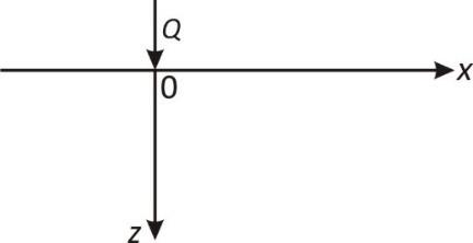
4.3 Line load Q in the elastic half-plane
4.3.1 Stress function for line load on elastic half-plane
Figure 1. Line load of intensity Q on an elastic half-plane
For the case of a line load of intensity Q, on an elastic half-plane as shown in Figure 1, the load function can be given by:
$p(x)=-\frac{Q}{2\in }$,$|x|<\epsilon$ (72)
$p(x)=0,|x|<\in$ (73)
where $\in \rightarrow 0$ and $\in$ is a small quantity.
Then,
$\begin{align} & {{A}_{1}}(\beta )=\frac{1}{\pi }\int\limits_{-\infty }^{\infty }{\frac{-Q}{2\in }\cos \beta t\,\,dt} \\ & =\frac{-2}{\pi }\int\limits_{0}^{\infty }{\frac{Q}{2\in }\cos \beta t\,dt}=\frac{-2}{\pi }\int\limits_{t=0}^{t=\in }{\frac{Q}{2\in }\cos \beta t\,dt} \\\end{align}$
$=\frac{-2Q}{2\pi \in }\int\limits_{0}^{\in }{\cos \beta t\,dt}=\frac{-Q}{\pi \in }\int\limits_{0}^{\in }{\cos \beta t\,dt}$ (74)
$=\frac{-Q}{\pi \in }\frac{\sin \beta \in }{\beta }=\frac{-Q}{\pi }\frac{\sin \beta \in }{\beta \in }$
${{A}_{2}}(\beta )=\frac{2}{\pi }\int\limits_{0}^{\infty }{\frac{-Q}{2\in }}\sin \beta t\,dt=0$ (75)
As $\in \rightarrow 0, \frac{\sin \beta \in}{\beta \in} \rightarrow 1$ and
${{A}_{1}}(\beta )=\frac{-Q}{\pi }$ (76)
${{A}_{2}}(\beta )=0$ (77)
\({{c}_{1}}(\beta )=\frac{-{{A}_{1}}(\beta )}{2G{{\beta }^{2}}}=-\frac{(-Q\text{/}\pi )}{2G{{\beta }^{2}}}=\frac{Q}{2\pi G{{\beta }^{2}}}\) (78)
${{c}_{2}}(\beta )=0$ (79)
The stress function is thus,
$\Omega (x,z)=\int\limits_{0}^{\infty }{\frac{Q}{2\pi G{{\beta }^{2}}}}\cos \beta x\exp (-\beta z)d\beta $ (80)
$\Omega (x,z)=\frac{Q}{2\pi G}\int\limits_{0}^{\infty }{\frac{\cos \beta x\exp (-\beta z)}{{{\beta }^{2}}}d\beta }$ (81)
This integral for the Love’s stress function for the 2D problem is divergent (does not converge).
However, by differentiation,
$\frac{{{\partial }^{2}}\Omega (x,z)}{\partial {{x}^{2}}}=\frac{{{\partial }^{2}}}{\partial {{x}^{2}}}\int\limits_{0}^{\infty }{\frac{Q}{2\pi G{{\beta }^{2}}}}\cos \beta x\exp (-\beta z)d\beta $ (82)
$\frac{{{\partial }^{2}}\Omega }{\partial {{x}^{2}}}=\frac{-Q}{2\pi G}\int\limits_{0}^{\infty }{\cos \beta x\exp (-\beta z)d\beta }$ (83)
The integral obtained for the function $\frac{\partial^{2} \Omega}{\partial x^{2}}(x, Z)$ converges, and can be readily evaluated.
Evaluation yields:
$\int\limits_{0}^{\infty }{\cos \beta x\exp (-\beta z)}\,d\beta =\frac{z}{{{x}^{2}}+{{z}^{2}}}$ (84)
Similarly,
$\frac{{{\partial }^{2}}\Omega }{\partial {{z}^{2}}}=\frac{Q}{2\pi G}\int\limits_{0}^{\infty }{\cos \beta x\exp (-\beta z)}\,d\beta $ (85)
$\frac{{{\partial }^{3}}\Omega }{\partial {{z}^{3}}}=\frac{Q}{2\pi G}\int\limits_{0}^{\infty }{-\beta \cos \beta x\exp (-\beta z)}\,d\beta $ (86)
$\frac{{{\partial }^{3}}\Omega }{\partial {{x}^{2}}\partial z}=\frac{Q}{2\pi G}\int\limits_{0}^{\infty }{\beta \cos \beta x\exp (-\beta z)}\,d\beta $ (87)
4.3.2 Stresses in elastic half-plane due to line load Q
The vertical stress field is then found using Eq. (55) as:
${{\sigma }_{zz}}=2G\left( z\frac{Q}{2\pi G}\int\limits_{0}^{\infty }{\begin{align} & -\beta \cos \beta x\exp (-\beta z) \\ & -\frac{Q}{2\pi G}\int\limits_{0}^{\infty }{\cos \beta x\exp (-\beta z)\,dz} \\ \end{align}} \right)$ (88)
Simplifying,
$\begin{align} & {{\sigma }_{zz}}=\frac{Qz}{\pi }\int\limits_{0}^{\infty }{-\beta \cos \beta x\exp (-\beta z)}\,dz \\ & -\frac{Q}{\pi }\int\limits_{0}^{\infty }{\cos \beta x\exp (-\beta z)dz} \\\end{align}$ (89)
Evaluating the integrals,
${{\sigma }_{zz}}=\frac{Qz}{\pi }\cdot \frac{{{x}^{2}}-{{z}^{2}}}{{{({{x}^{2}}+{{z}^{2}})}^{2}}}-\frac{Q}{\pi }\frac{z}{({{x}^{2}}+{{z}^{2}})}$ (90)
Further simplification yields:
\({{\sigma }_{zz}}=\frac{Q}{\pi }\left( \frac{2({{x}^{2}}-{{z}^{2}})}{{{({{x}^{2}}+{{z}^{2}})}^{2}}}-\frac{z}{({{x}^{2}}+{{z}^{2}})} \right)\) (91)
Simplifying further,
\({{\sigma }_{zz}}=\frac{Q}{\pi }\left( \frac{2({{x}^{2}}-{{z}^{2}})-z({{x}^{2}}+{{z}^{2}})}{{{({{x}^{2}}+{{z}^{2}})}^{2}}} \right)\) (92)
Simplifying,
\({{\sigma }_{zz}}=\frac{Q}{\pi }\left( \frac{{{x}^{2}}z-{{z}^{3}}-{{x}^{2}}z-{{z}^{3}})}{{{({{x}^{2}}+{{z}^{2}})}^{2}}} \right)\) (93)
Further simplification gives:
${{\sigma }_{zz}}=\frac{-2Q}{\pi }\frac{{{z}^{3}}}{{{({{x}^{2}}+{{z}^{2}})}^{2}}}$ (94)
Similarly, $\sigma_{x x}(x, Z)$ is found from Eq. (56) is follows:
\({{\sigma }_{xx}}=2G\left\{ (1-2\mu )\left( -\frac{Q}{2\pi G} \right)\int\limits_{0}^{\infty }{\cos \beta x\exp (-\beta z)d\beta +} \right.\)
\(\frac{z\cdot Q}{2\pi G}\int\limits_{0}^{\infty }{\beta \cos \beta x\exp (-\beta z)d\beta }-\)$\left. \frac{2\mu Q}{2\pi G}\int\limits_{0}^{\infty }{\cos \beta x\exp (-\beta z)d\beta } \right\}$ (95)
Simplifying, we have:
$\begin{align} & {{\sigma }_{xx}}=\frac{-Q(1-2\mu )}{\pi }\int\limits_{0}^{\infty }{\cos \beta x\exp (-\beta z)}d\beta \\ & +\frac{Qz}{\pi }\int\limits_{0}^{\infty }{\beta \cos \beta x\exp (-\beta z)}d\beta - \\\end{align}$ (96)
$\frac{2\mu Q}{\pi }\int\limits_{0}^{\infty }{\cos \beta x}\exp (-\beta z)d\beta $
Evaluating, the integrals, we obtain:
$\begin{align} & {{\sigma }_{xx}}=\frac{-Q(1-2\mu )}{\pi }\frac{z}{({{x}^{2}}+{{z}^{2}})} \\ & +\frac{Qz}{\pi }\left( \frac{{{z}^{2}}-{{x}^{2}}}{{{({{x}^{2}}+{{z}^{2}})}^{2}}} \right)-\frac{2\pi Q}{\pi }\frac{z}{{{x}^{2}}+{{z}^{2}}} \\\end{align}$ (97)
Simplifying,
$\begin{align} & {{\sigma }_{xx}}=\left( -\frac{Q}{\pi }+\frac{2\mu Q}{\pi } \right)\frac{z}{{{x}^{2}}+{{z}^{2}}} \\ & +\frac{Qz}{\pi }\left( \frac{{{z}^{2}}-{{x}^{2}}}{{{x}^{2}}+{{z}^{2}}} \right)-\frac{2\mu Q}{\pi }\frac{z}{{{x}^{2}}+{{z}^{2}}} \\\end{align}$ (98)
Simplifying,
${{\sigma }_{xx}}=\frac{-Q}{\pi }\frac{z}{{{x}^{2}}+{{z}^{2}}}+\frac{Qz}{\pi }\left( \frac{{{z}^{2}}-{{x}^{2}}}{{{({{x}^{2}}+{{z}^{2}})}^{2}}} \right)$ (99)
Simplifying,
\({{\sigma }_{xx}}=\frac{Q}{\pi }\left( \frac{z({{z}^{2}}-{{x}^{2}})}{{{({{x}^{2}}+{{z}^{2}})}^{2}}}-\frac{z}{{{x}^{2}}+{{z}^{2}}} \right)\) (100)
Simplifying further,
${{\sigma }_{xx}}=\frac{Q}{\pi }\left( \frac{z({{z}^{2}}-{{x}^{2}})-z({{x}^{2}}+{{z}^{2}})}{{{({{x}^{2}}+{{z}^{2}})}^{2}}} \right)$ (101)
Simplifying,
${{\sigma }_{xx}}=\frac{Q}{\pi }\left( \frac{{{z}^{3}}-z{{x}^{2}}-z{{x}^{2}}-{{z}^{3}}}{{{({{x}^{2}}+{{z}^{2}})}^{2}}} \right)$ (102)
Simplifying,
${{\sigma }_{xx}}=\frac{Q}{\pi }\left( \frac{-2z{{x}^{2}}}{{{({{x}^{2}}+{{z}^{2}})}^{2}}} \right)$ (103)
Hence,
${{\sigma }_{xx}}=\frac{-2Qz{{x}^{2}}}{{{({{x}^{2}}+{{z}^{2}})}^{2}}}$
$\tau_{x y}=0, \tau_{y z}=0$ (104)
The stresses are expressed in terms of the 2D polar coordinates using the coordinate transformations:
$x=r\cos \theta $ (105)
$z=r\sin \theta $ (106)
${{x}^{2}}+{{z}^{2}}={{r}^{2}}$ (107)
$\frac{x}{r}=\cos \theta $ (108)
$\frac{z}{r}=\sin \theta $ (109)
Then,
${{\sigma }_{xx}}=\frac{-2Q}{\pi r}{{\cos }^{2}}\theta \sin \theta $ (110)
${{\sigma }_{zz}}=\frac{-2Q}{\pi r}{{\sin }^{3}}\theta $ (111)
${{\tau }_{xz}}=\frac{-2Q}{\pi r}{{\sin }^{2}}\theta \cos \theta $ (112)
The stress components in polar coordinates are:
${{\sigma }_{rr}}={{\sigma }_{xx}}{{\cos }^{2}}\theta +{{\sigma }_{zz}}{{\sin }^{2}}\theta +{{\tau }_{xz}}\sin 2\theta $ (113)
${{\sigma }_{\theta \theta }}={{\sigma }_{zz}}{{\cos }^{2}}\theta +{{\sigma }_{xx}}{{\sin }^{2}}\theta -{{\tau }_{xz}}\sin 2\theta $ (114)
${{\tau }_{r\theta }}=({{\sigma }_{zz}}-{{\sigma }_{xx}})\sin \theta \cos \theta +{{\tau }_{xz}}\cos 2\theta $ (115)
${{\sigma }_{rr}}=\frac{-2Q}{\pi r}\sin \theta =\frac{-2Qz}{\pi {{r}^{2}}}$ (116)
${{\sigma }_{\theta \theta }}=0$ (117)
${{\tau }_{r\theta }}=0$ (118)
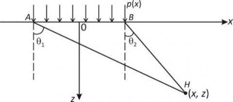
4.4 Strip load of finite width on the elastic half-plane
For a strip load of width 2b as shown in Figure 2, the origin, O, and arbitrary point, H is the elastic half-plane are shown in the Figure 2.
Figure 2. Strip load of finite width on the elastic half-plane
The Fourier integral of the load p(x) is given by:
$p(x)=\int\limits_{-\infty }^{\infty }{({{A}_{1}}(\beta )\cos \beta x+{{A}_{2}}(\beta )\sin \beta x)d\beta }$ (119)
where,
${{A}_{1}}(\beta )=\frac{1}{\pi }\int\limits_{-\infty }^{\infty }{p(t)\cos \beta t\,dt}=\frac{2}{\pi }\int\limits_{0}^{\infty }{p(t)\cos \beta t\,dt}$ (120)
${{A}_{2}}(\beta )=\frac{1}{\pi }\int\limits_{-\infty }^{\infty }{p(t)\sin \beta t\,dt}=\frac{2}{\pi }\int\limits_{0}^{\infty }{p(t)\sin \beta t\,dt}$ (121)
For a uniformly distributed strip load of intensity q, we have:
$p(x)=-q|x|<b, p(x)=0|x|>b$, then,
${{A}_{1}}(\beta )=\frac{2}{\pi }\int\limits_{0}^{\infty }{q\cos \beta t\,dt}$ (122)
${{A}_{1}}(\beta )=\frac{2}{\pi }\int\limits_{0}^{b}{q\cos \beta t\,dt}$ (123)
${{A}_{1}}(\beta )=\frac{2}{\pi }q\left[ \frac{\sin \beta t}{\beta } \right]_{0}^{b}$ (124)
${{A}_{1}}(\beta )=\frac{2q}{\pi }\frac{\sin \beta b}{\beta }$ (125)
$\begin{align} & {{A}_{2}}(\beta )=\frac{2}{\pi }\int\limits_{0}^{\infty }{q\sin \beta t\,dt}=\frac{2}{\pi }\int\limits_{0}^{b}{q\sin \beta t\,dt} \\ & =\frac{2q}{\pi }\int\limits_{0}^{b}{\sin \beta t\,dt}=\frac{2q}{\pi }\left[ \frac{-\cos \beta t}{\beta } \right]_{0}^{b} \\\end{align}$ (126)
${{A}_{2}}(\beta )=\frac{-2q}{\pi }\frac{\cos \beta b}{\beta }$ (127)
Hence,
${{c}_{1}}(\beta )=\frac{-{{A}_{1}}(\beta )}{2G{{\beta }^{2}}}=\frac{-2q}{\beta }\frac{\sin \beta b}{2G{{\beta }^{2}}}$ (128)
${{c}_{2}}(\beta )=\frac{-{{A}_{2}}(\beta )}{2G{{\beta }^{2}}}=\frac{2q}{\pi }\frac{\cos \beta b}{\beta 2G{{\beta }^{2}}}=\frac{2q\cos \beta b}{2\pi G{{\beta }^{3}}}$ (129)
The Love stress function for the case of uniformly distributed strip load is then:
$\begin{align} & \Omega (x,z) \\ & =\int\limits_{0}^{\infty }{\left( \frac{-2q\sin \beta b}{2\pi G{{\beta }^{3}}}\cos \beta x+\frac{2q\cos \beta b\sin \beta x}{2\pi G{{\beta }^{3}}} \right)}\,{{e}^{-\beta z}}d\beta \\\end{align}$ (130)
Simplifying,
$\Omega =\frac{q}{\pi G}\int\limits_{0}^{\infty }{\left( \frac{\cos \beta b}{{{\beta }^{3}}}\sin \beta x-\frac{\sin \beta b\cos \beta x}{{{\beta }^{3}}} \right)}\,{{e}^{-\beta z}}d\beta $ (131)
Further simplification yields
$\Omega =\frac{q}{\pi G}\int\limits_{0}^{\infty }{\frac{(\cos \beta b\sin \beta x-\sin \beta b\cos \beta x)}{{{\beta }^{3}}}}\,{{e}^{-\beta z}}d\beta $ (132)
Using trigonometric identities,
$\Omega =\frac{q}{\pi G}\int\limits_{0}^{\infty }{\frac{\sin (\beta x-\beta b)}{{{\beta }^{3}}}}\,{{e}^{-\beta z}}d\beta $ (133)
Simplifying,
$\Omega =\frac{q}{\pi G}\int\limits_{0}^{\infty }{\frac{\sin \beta (x-b)}{{{\beta }^{3}}}}\,\exp (-\beta z)d\beta $ (134)
By differentiation of $\Omega(x, z)$ with respect to z, we have:
$\frac{\partial \Omega }{\partial z}=\frac{q}{\pi G}\int\limits_{0}^{\infty }{\frac{\sin \beta (x-b)}{{{\beta }^{3}}}}\frac{d}{dz}{{e}^{-\beta z}}d\beta $ (135)
Simplifying,
$\frac{\partial \Omega }{\partial z}=\frac{q}{\pi G}\int\limits_{0}^{\infty }{\frac{\sin \beta (x-b)}{{{\beta }^{3}}}}(-\beta {{e}^{-\beta z}})d\beta $ (136)
Further simplification yields:
$\frac{\partial \Omega }{\partial z}=\frac{q}{\pi G}\int\limits_{0}^{\infty }{\frac{-\sin \beta (x-b)}{{{\beta }^{2}}}}{{e}^{-\beta z}}d\beta $ (137)
Differentiation of Eq. (137) again with respect to z yields:
$\frac{{{\partial }^{2}}\Omega }{\partial {{z}^{2}}}=\frac{q}{\pi G}\int\limits_{0}^{\infty }{\frac{-\sin \beta (x-b)}{{{\beta }^{2}}}}\frac{\partial }{\partial z}{{e}^{-\beta z}}d\beta $ (138)
Simplifying,
$\frac{{{\partial }^{2}}\Omega }{\partial {{z}^{2}}}=\frac{q}{\pi G}\int\limits_{0}^{\infty }{\frac{-\sin \beta (x-b)}{{{\beta }^{2}}}}-(\beta {{e}^{-\beta z}})d\beta $ (139)
Simplifying,
$\frac{{{\partial }^{2}}\Omega }{\partial {{z}^{2}}}=\frac{q}{\pi G}\int\limits_{0}^{\infty }{\frac{\sin \beta (x-b)}{\beta }}{{e}^{-\beta z}}d\beta $ (140)
By differentiation of Eq. (140) with respect to z, we have;
$\frac{{{\partial }^{3}}\Omega }{\partial {{z}^{3}}}=\frac{q}{\pi G}\int\limits_{0}^{\infty }{\frac{\sin \beta (x-b)}{\beta }}\frac{\partial }{\partial z}{{e}^{-\beta z}}d\beta $ (141)
Simplifying,
$\frac{{{\partial }^{3}}\Omega }{\partial {{z}^{3}}}=\frac{q}{\pi G}\int\limits_{0}^{\infty }{\frac{\sin \beta (x-b)}{\beta }}(-\beta {{e}^{-\beta z}})d\beta $ (142)
Further simplification yields:
$\frac{{{\partial }^{3}}\Omega }{\partial {{z}^{3}}}=\frac{q}{\pi G}\int\limits_{0}^{\infty }{-\sin \beta (x-b)\,}{{e}^{-\beta z}}d\beta $ (143)
Differentiation of the Love stress function with respect to x yields:
$\frac{\partial \Omega }{\partial x}=\frac{q}{\pi G}\int\limits_{0}^{\infty }{\frac{\partial }{\partial x}\sin \beta (x-b)}\frac{1}{{{\beta }^{3}}}{{e}^{-\beta z}}d\beta $ (144)
Simplifying,
\(\frac{\partial \Omega }{\partial x}=\frac{q}{\pi G}\int\limits_{0}^{\infty }{\frac{\beta \cos \beta (x-b)}{{{\beta }^{3}}}}{{e}^{-\beta z}}d\beta \) (145)
By differentiation of Eq. (145), we have:
$\frac{{{\partial }^{2}}\Omega }{\partial {{x}^{2}}}=\frac{q}{\pi G}\int\limits_{0}^{\infty }{\frac{\partial }{\partial x}\frac{\cos \beta (x-b)}{{{\beta }^{2}}}\,}{{e}^{-\beta z}}d\beta $ (146)
Simplifying,
$\frac{{{\partial }^{2}}\Omega }{\partial {{x}^{2}}}=\frac{q}{\pi G}\int\limits_{0}^{\infty }{\frac{-\beta \sin \beta (x-b)}{{{\beta }^{2}}}}{{e}^{-\beta z}}d\beta $ (147)
Simplifying,
\(\frac{{{\partial }^{2}}\Omega }{\partial {{x}^{2}}}=\frac{q}{\pi G}\int\limits_{0}^{\infty }{\frac{-\sin \beta (x-b)}{\beta }}{{e}^{-\beta z}}d\beta \) (148)
Differentiation of Eq. (148) with respect to z yield:
$\frac{{{\partial }^{3}}\Omega }{\partial {{x}^{2}}\partial z}=\frac{q}{\pi G}\int\limits_{0}^{\infty }{\frac{-\sin \beta (x-b)}{{{\beta }^{2}}}\,}\frac{d}{dz}{{e}^{-\beta z}}d\beta $ (149)
Simplifying,
$\frac{{{\partial }^{3}}\Omega }{\partial {{x}^{2}}\partial z}=\frac{q}{\pi G}\int\limits_{0}^{\infty }{\frac{-\sin \beta (x-b)}{\beta }(-\beta }{{e}^{-\beta z}})d\beta $ (150)
Simplifying,
$\frac{{{\partial }^{3}}\Omega }{\partial {{x}^{2}}\partial z}=\frac{q}{\pi G}\int\limits_{0}^{\infty }{\sin \beta (x-b)}{{e}^{-\beta z}}d\beta $ (151)
Differentiation of Eq. (138) with respect to x yields:
$\frac{{{\partial }^{3}}\Omega }{\partial x\partial {{z}^{2}}}=\frac{q}{\pi G}\int\limits_{0}^{\infty }{\frac{\partial }{\partial x}\frac{\sin \beta (x-b)}{\beta }\,}{{e}^{-\beta z}}d\beta $ (152)
Simplifying,
$\frac{{{\partial }^{3}}\Omega }{\partial x\partial {{z}^{2}}}=\frac{q}{\pi G}\int\limits_{0}^{\infty }{\frac{\beta \cos \beta (x-b)}{\beta }}{{e}^{-\beta z}}d\beta $ (153)
Simplifying,
$\frac{{{\partial }^{3}}\Omega }{\partial x\partial {{z}^{2}}}=\frac{q}{\pi G}\int\limits_{0}^{\infty }{\cos \beta (x-b)}{{e}^{-\beta z}}d\beta $ (154)
Stress fields for strip loads
Evaluating the integrals and using the Love stress functions, the stress fields for strip heads are obtained as follows:
\({{\sigma }_{zz}}=\frac{q}{\pi }\left[ \begin{align} & {{\tan }^{-1}}\left( \frac{z}{x-b} \right) \\ & -{{\tan }^{-1}}\left( \frac{z}{x+b} \right)-\frac{2bz({{x}^{2}}-{{z}^{2}}-{{b}^{2}})}{{{({{x}^{2}}+{{z}^{2}}-{{b}^{2}})}^{2}}+4{{b}^{2}}{{z}^{2}}} \\\end{align} \right]\) (155)
\({{\sigma }_{xx}}=\frac{q}{\pi }\left[ \begin{align} & {{\tan }^{-1}}\left( \frac{z}{x-b} \right) \\ & -{{\tan }^{-1}}\left( \frac{z}{x+b} \right)+\frac{2bz({{x}^{2}}-{{z}^{2}}-{{b}^{2}})}{{{({{x}^{2}}+{{z}^{2}}-{{b}^{2}})}^{2}}+4{{b}^{2}}{{z}^{2}}} \\\end{align} \right]\) (156)
${{\tau }_{xz}}=\frac{q}{\pi }\left( \frac{4bx{{z}^{2}}}{{{({{x}^{2}}+{{z}^{2}}-{{b}^{2}})}^{2}}+4{{b}^{2}}{{z}^{2}}} \right)$ (157)
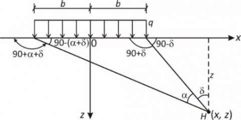
or, in simplified trigonometric forms,
${{\sigma }_{zz}}=\frac{q}{\pi }(\alpha +\sin \alpha \cos (\alpha +2\delta ))$ (158)
${{\sigma }_{xx}}=\frac{q}{\pi }(\alpha -\sin \alpha \cos (\alpha +2\delta ))$ (159)
${{\tau }_{xz}}=\frac{q}{\pi }(\sin \alpha \sin (\alpha +2\delta ))$ (160)
where, the angles, a and d are defined as shown in Figure 3.
Figure 3. Uniformly distributed vertical infinitely long strip load of width 2b acting on the surface of an elastic semi-infinite soil mass
$\tan (90-\delta )=\frac{z}{x-b}$ (161)
$\tan 90-(\alpha +\delta )=\frac{z}{x+b}$ (162)
$90-\delta ={{\tan }^{-1}}\left( \frac{z}{x-b} \right)$ (163)
$90-(\alpha +\delta )={{\tan }^{-1}}\left( \frac{z}{x+b} \right)$ (164)
$90-\delta -(90-(\alpha +\delta ))=90-\delta -90+(\alpha +\delta )$$=\alpha +\delta -\delta =\alpha $ (165)
$\alpha ={{\tan }^{-1}}\left( \frac{z}{x-b} \right)-{{\tan }^{-1}}\left( \frac{z}{x+b} \right)$ (166)
The results are presented in non-dimensional forms in Tables 1, 2, and 3 for the various loading cases considered in this study. The results are further validated in Table 3 which compared the present results with previous results and illustrates the agreement of present results with the previous results of Das [2] and Onah et al. [13].
Table 1. Non-dimensional vertical stress influence values for line load on elastic half-plane Values of szz/q, sxx/q, and txz/q for vertical strip loading
|
x/b |
z/b |
szz/q |
sxx/q |
txz/q |
x/b |
z/b |
szz/q |
sxx/q |
txz/q |
|
0 |
0 0.5 1.0 1.5 2.0 2.5 |
1.000 0.9594 0.8183 0.6678 0.5508 0.4617 |
1.000 0.4498 0.1817 0.0803 0.0410 0.0228 |
0 0 0 0 0 0 |
1.5 |
0.25 0.5 1.0 1.5 2.0 2.5 |
0.0177 0.0892 0.2488 0.2704 0.2876 0.2851 |
0.2079 0.2850 0.2137 0.1807 0.1268 0.0892 |
0.0606 0.1466 0.2101 0.2022 0.1754 0.1469 |
|
|
|
|
|
|
|
|
|
|
|
|
0.5 |
0 0.25 0.5 1.0 1.5 2.0 2.5 |
1.000 0.9787 0.9028 0.7352 0.6078 0.5107 0.4372 |
1.000 0.6214 0.3920 0.1863 0.0994 0.0542 0.0334 |
0 0.0522 0.1274 0.1590 0.1275 0.0959 0.0721 |
2.0 |
0.25 0.5 1.0 1.5 2.0 2.5 |
0.0027 0.0194 0.0776 0.1458 0.1847 0.2045 |
0.0987 0.1714 0.2021 0.1847 0.1456 0.1256 |
0.0164 0.0552 0.1305 0.1568 0.1567 0.1442 |
|
|
|
|
|
|
|
|
|
|
|
|
1.0 |
0.25 0.5 1.0 1.5 2.0 2.5 |
0.4996 0.4969 0.4797 0.4480 0.4095 0.3701 |
0.4208 0.3472 0.2250 0.1424 0.0908 0.0595 |
0.3134 0.2996 0.2546 0.2037 0.1592 0.1243 |
2.5 |
0.5 1.0 1.5 2.0 2.5 |
0.0068 0.0357 0.0771 0.1139 0.1409 |
0.1104 0.1615 0.1645 0.1447 0.1205 |
0.0254 0.0739 0.1096 0.1258 0.1266 |
Table 2. Dimensionless influence values for uniformly distributed strip load on elastic half-plane
|
szz/q |
|||||||||||
|
(x/b) |
|||||||||||
|
(z/b) |
0.0 |
0.1 |
0.2 |
0.3 |
0.4 |
0.5 |
0.6 |
0.7 |
0.8 |
0.9 |
1.0 |
|
0.00 0.10 0.20 0.30 0.40 0.50 0.60 0.70 0.80 0.90 1.00 1.10 1.20 1.30 1.40 1.50 1.60 1.70 1.80 |
1.000 1.000 0.997 0.990 0.977 0.959 0.937 0.910 0.881 0.850 0.818 0.787 0.755 0.725 0.696 0.668 0.642 0.617 0.593 |
1.000 1.000 0.997 0.989 0.976 0.958 0.935 0.908 0.878 0.847 0.815 0.783 0.752 0.722 0.693 0.666 0.639 0.615 0.591 |
1.000 0.999 0.996 0.987 0.973 0.953 0.928 0.899 0.869 0.837 0.805 0.774 0.743 0.714 0.685 0.658 0.633 0.608 0.585 |
1.000 0.999 0.995 0.984 0.966 0.943 0.915 0.885 0.853 0.821 0.789 0.758 0.728 0.699 0.672 0.646 0.621 0.598 0.576 |
1.000 0.999 0.992 0.978 0.955 0.927 0.896 0.863 0.829 0.797 0.766 0.735 0.707 0.679 0.653 0.629 0.605 0.583 0.563 |
1.000 0.998 0.988 0.967 0.937 0.902 0.866 0.831 0.797 0.765 0.735 0.706 0.679 0.654 0.630 0.607 0.586 0.565 0.546 |
1.000 0.997 0.979 0.947 0.906 0.864 0.825 0.788 0.755 0.724 0.696 0.670 0.646 0.623 0.602 0.581 0.562 0.544 0.526 |
1.000 0.993 0.959 0.908 0.855 0.808 0.767 0.732 0.701 0.675 0.650 0.628 0.607 0.588 0.569 0.552 0.535 0.519 0.504 |
1.000 0.980 0.909 0.833 0.773 0.727 0.691 0.662 0.638 0.617 0.598 0.580 0.564 0.548 0.534 0.519 0.506 0.492 0.479 |
1.000 0.909 0.775 0.697 0.651 0.620 0.598 0.581 0.566 0.552 0.540 0.529 0.517 0.506 0.495 0.484 0.474 0.463 0.453 |
0.000 0.500 0.500 0.499 0.498 0.497 0.495 0.492 0.489 0.485 0.480 0.474 0.468 0.462 0.455 0.448 0.440 0.433 0.425 |
Table 3. Variation of szz/(q/z) with x/z
|
x/z |
Present study szz/(q/z) |
Reference [2, 13] szz/(q/z) |
x/z |
Present study szz/(q/z) |
Reference [2, 13] szz/(q/z) |
|
0 0.1 0.2 0.3 0.4 0.5 0.6 0.7 0.8 0.9 1.0 1.1 1.2 |
0.637 0.624 0.589 0.536 0.473 0.407 0.344 0.287 0.237 0.194 0.159 0.130 0.107 |
0.637 0.624 0.589 0.536 0.473 0.407 0.344 0.287 0.237 0.194 0.159 |
1.3 1.4 1.5 1.6 1.7 1.8 1.9 2.0 2.2 2.4 2.6 2.8 3.0 |
0.088 0.073 0.060 0.050 0.042 0.035 0.030 0.025 0.019 0.014 0.011 0.008 0.006 |
0.060
0.025
0.006 |
The Fourier integral method was successfully used in this work to determine the normal and shear stress fields in an elastic half-plane under line and strip loads applied on the boundary. The elastic half-plane is made of soil that is assumed linear elastic, isotropic, homogeneous and of semi-infinite extent with $-\infty \leq x \leq \infty, 0 \leq z \leq \infty$. The governing equations of the elastic half-plane problem are the differential equations of equilibrium, the stress compatibility equation, the geometric (strain –displacement) relations and the boundary conditions. Stress formulation of the equations was adopted and the Beltrami – Michell stress compatibility equation was formulated for the two dimensional elastic half-plane problem considered. The Fourier integral transformation method was applied to the governing Beltrami – Michell stress compatibility equation in Eq. (46) to transform the problem from a boundary value problem to a fourth order linear ordinary differential equation (Eq. (49)) in terms of the stress functions in the Fourier integral transform space variable. The fourth order ODE was solved using methods for solving ODEs to obtain the stress function in the Fourier integral space in terms of four integration constants as Eq. (50). By inversion of Eq. (50), the stress function was obtained in the physical domain space variables as Eq. (51) which contained four unknown integration constants, $c_{1}(\beta), c_{2}(\beta), c_{3}(\beta)$ and $c_{4}(\beta)$, which in general are functions of the Fourier integral parameter $\beta$. The requirements for boundedness of the stresses and hence the stress functions were used to obtain solutions to two of the unknown constants of integration as Eqns. (52) and (53); thus, simplifying the unknown stress function as Equation (54) which had two unknown integration constants. Love stress functions for plane elasticity problems given as Eqns. (55) – (60) were used to obtain the expressions for the Cartesian stress components. The general problem of distributed load p(x) applied to the surface of the elastic half-plane was considered and the equilibrium of internal vertical stresses and the external (applied) stresses on the surface z = 0 was used to obtain the boundary conditions as Eq. (64). The enforcement of the boundary conditions gave the values of the two unknown integration constants for the bounded stress functions as Eqns. (68) and (69). For the case of line load of intensity Q, described mathematically as Eqns. (72) and (73), the unknown integration constants were found as Eqns. (76) and (77) or (78) and (79). The bounded Love stress function for the case of line load of intensity Q was then found as Eq. (81). The obtained expression for the Love stress function for line load was then used in Eqns. (55) – (60) to obtain the Cartesian stress components respectively as Eqns. (94) and (104). The stresses were expressed in terms of plane polar coordinates to obtain Eqns. (110) – (112).
For the case of strip load of intensity q and finite width 2b, considered as shown in Figures 2 and 3, the equilibrium of the internal vertical stresses and the external stresses on the z = 0 plane was used as the boundary condition to obtain the unknown integration constants as Eqns. (128) and (129). The bounded Love stress functions for the finite strip load of uniform intensity was thus obtained as Eq. (134). The Love stress function expressions Eqns. (55 – 60) were used to obtain the Cartesian stress components for the elastic half-plane problem under finite strip load as Eqns. (155) for $\sigma_{z z}$, (156) for $\sigma_{x x}$, and (157) for $\tau_{x z}$. The stresses were presented in trigonometric forms respectively as Eqns. (158 – 160).
It was observed that the expressions obtained for the Cartesian stress field components $\sigma_{x x}, \sigma_{z z}$ and $\tau_{x z}$ were identical for the two particular cases considered – line load and finite width strip load of uniform intensity – to the expressions obtained by Das [2], Onah et al. [13] and other researchers, who solved the elastic half-plane problem using other methods such as the displacement based approach, or Airy stress function method. Eqns. (155-157) were calculated for different various values of x/b and z/b and the influence values for the normal and shear stresses for strip load of finite width (2b) presented as Tables 1 and 2. Similarly, the influence values for vertical stress due to line load of constant intensity Q were evaluated and presented for various values of x/z as Table 3.
The conclusions of the present work are as follows:
(i) The Fourier integral method has been successfully used in this work to obtain general solutions for bounded Love stress functions, and normal ($\sigma_{x x}, \sigma_{z z}$) and shear stresses $\tau \mathrm{xZ}$ in a linear elastic, isotropic, homogeneous elastic half-plane in the xz coordinate for $-\infty \leq x \leq \infty ; \quad 0 \leq z \leq \infty$ under distributed boundary load p(x).
(ii) The Fourier integral method has been successfully used in this work to obtain solutions for bounded Love stress functions, Cartesian stress field components $\sigma_{x x}, \sigma_{z z}, \tau_{x z}$ is an elastic half-plane due to line load of uniform intensity Q applied on the surface.
(iii) The Fourier integral transform method has been used in this work to obtain bounded Love stress functions, and Cartesian stress field components $\sigma_{x x}, \sigma_{z z}$ and $\tau_{x z}$ in elastic half-plane problems due to finite width strip loads of constant intensity applied on the boundary.
(iv) The Fourier integral method transforms the elastic half-plane problem expressed in stress formulation using Beltrami – Michell stress compatibility equations to a linear ordinary differential equation in terms of the unknown stress function $\bar{\Omega}(\beta, z)$ expressed in terms of the Fourier integral transform space variables.
(v) The stress formulation method adopted in this work simplified the elastic half-plane problem to a problem of finding a suitable biharmonic stress function $\Omega(\mathrm{x}, \mathrm{z})$ that satisfies the boundary conditions of the particular (given) elastic half-plane problem expressed by the equilibrium of internal vertical stresses and the external stresses/load at the z=0 plane.
(vi) The resulting solutions obtained for the Love stress functions and the Cartesian stress field components satisfy the boundedness conditions at $Z \rightarrow \infty$, and are bounded solutions.
(vii) The Fourier integral method is an integral transformation method which transforms the governing Beltrami – Michell stress compatibility equation, a biharmonic partial differential equation in terms of the stress function to an ordinary differential equation (ODE) which would be more amenable to closed form mathematical solutions.
|
2D |
two dimensional |
|
ODE |
Ordinary Differential Equation |
|
ODEs |
Ordinary Differential Equations |
|
x, y, z |
Cartesian coordinates |
|
2a (or 2b) |
width of a finite strip load |
|
$\mathcal{E}_{x x}$ |
normal strain in the x direction |
|
${{\varepsilon }_{yy}}$ |
normal strain in the y direction |
|
${{\varepsilon }_{zz}}$ |
normal strain in the z direction |
|
u |
displacement component in the x direction |
|
v |
displacement component in y direction |
|
w |
displacement component in z direction |
|
${{\varepsilon }_{xz}},{{\varepsilon }_{yz}},{{\varepsilon }_{xy}}$ |
normal strains |
|
$\begin{align} & {{\tau }_{xy}},{{\tau }_{yz}},{{\tau }_{xz}} \\ & {{\sigma }_{xz}},{{\sigma }_{yz}},{{\sigma }_{xz}} \\\end{align}$ |
shear stresses |
|
G |
shear modulus |
|
$\lambda$ |
Lamé’s constant |
|
fx, fy, fz |
body force components |
|
E |
Modulus of elasticity |
|
tx, tz |
tractions |
|
nx, nz |
direction cosines |
|
V |
potential function for the body forces |
|
$C(\mu )$ |
parameter defined in terms of $\mu$ for plane stress and plane strain elasticity |
|
$\frac{\partial }{\partial x},\frac{\partial }{\partial y},\frac{\partial }{\partial z}$ |
partial differential operators with respect to x, y and z respectively |
|
a1, a2, a3, a4 |
integration constants |
|
${{c}_{1}}(\beta ),{{c}_{2}}(\beta ),{{c}_{3}}(\beta ),{{c}_{4}}(\beta )$ |
four unknown functions of the Fourier integral tranform |
|
${{\bar{c}}_{1}},{{\bar{c}}_{2}}$ |
constants used in defining Fourier integral tranforms of the Airy stress function $\Omega (x,z)$ |
|
p(x) |
distributed load on the boundary of elastic half plane |
|
${{A}_{1}}(\beta ),{{A}_{2}}(\beta )$ |
constants used in defining the Fourier integral tranform of the distributed load p(x) |
|
t |
dummy variable of integration for integrals in respect of the distributed load |
|
$\in$ |
small quantity used in defining the line load |
|
q |
intensity of uniformly distributed strip load |
|
Greek symbols |
|
|
${{\nabla }^{2}}$ |
Laplace differential operator |
|
$\mu $ |
Poisson’s ratio |
|
$\varphi (x,z)$ |
Airy stress function for elasticity problems in the xz coordinate plane |
|
${{\nabla }^{4}}$ |
biharmonic differential operator |
|
$\nabla $ |
gradient operator |
|
$\beta $ |
Fourier integral tranform parameters |
|
$\Omega (x,z)$ |
Airy stress potential function adopted for the 2D elasticity problem studied |
|
$\bar{\Omega }(\beta ,z)$ |
Fourier integral transform of the stress function adopted for the 2D elasticity problem studied |
|
$\alpha ,\delta $ |
angles defined for the strip load problem shown in Figure 3. |
APPENDIX I
$\int\limits_{0}^{\infty }{{{e}^{\alpha y}}\cos (\alpha )}d\alpha =\frac{-y}{{{x}^{2}}+{{y}^{2}}}$
\[\int\limits_{0}^{\infty }{{{e}^{\alpha y}}\alpha \cos (\alpha x)}\,d\alpha =\frac{d}{dy}\int\limits_{0}^{\infty }{{{e}^{\alpha y}}\cos \alpha x}\,d\alpha =\frac{d}{dy}\left( \frac{-y}{{{x}^{2}}+{{y}^{2}}} \right)\]
\[\int\limits_{0}^{\infty }{{{e}^{\alpha y}}\alpha \sin \alpha x}\,d\alpha =\frac{-d}{dx}\int\limits_{0}^{\infty }{{{e}^{\alpha y}}\cos \alpha x}\,d\alpha =\frac{-d}{dx}\left( \frac{-y}{{{x}^{2}}+{{y}^{2}}} \right)=\frac{d}{dx}\left( \frac{y}{{{x}^{2}}+{{y}^{2}}} \right)\]
$\frac{{{\partial }^{3}}\Omega }{\partial x\partial {{z}^{2}}}=\frac{Q}{2\pi G}\int\limits_{0}^{\infty }{-\beta \sin \beta x\exp }(-\beta z)d\beta $
\[\int\limits_{0}^{\infty }{-\beta \cos \beta x\exp (-\beta z)d\beta }=\frac{{{x}^{2}}-{{z}^{2}}}{{{({{x}^{2}}+{{z}^{2}})}^{2}}}\]
Then, for line load q of infinite extent, the stress field are:
${{\sigma }_{xx}}=\frac{-2Q}{\pi }\frac{{{x}^{2}}z}{{{({{x}^{2}}+{{z}^{2}})}^{2}}}$
${{\sigma }_{zz}}=\frac{-2Q}{\pi }\frac{{{z}^{3}}}{{{({{x}^{2}}+{{z}^{2}})}^{2}}}$
${{\tau }_{xz}}=\frac{-2Q}{\pi }\frac{x{{z}^{2}}}{{{({{x}^{2}}+{{z}^{2}})}^{2}}}$
APPENDIX II
Solution to Eq. (49)
$\frac{{{d}^{4}}}{d{{z}^{4}}}\bar{\Omega }(\beta ,z)-2{{\beta }^{2}}\frac{{{d}^{2}}}{d{{z}^{2}}}\Omega (\beta ,z)+{{\beta }^{4}}\bar{\Omega }(\beta ,z)=0$
By the method of trial functions, the unknown $\bar{\Omega }(\beta ,z)$ is assumed to be an exponential function of z of the form:
$\bar{\Omega }(\beta ,z)=\exp \lambda z$
where, $\lambda $ is a parameter sought to enable the assumed trial exponential function be the desired solution.
Then,
$\frac{{{d}^{2}}}{d{{z}^{2}}}\bar{\Omega }(\beta ,z)={{\lambda }^{2}}\exp \lambda z$
$\frac{{{d}^{4}}}{d{{z}^{4}}}\bar{\Omega }(\beta ,z)={{\lambda }^{4}}\exp \lambda z$
Then the equation becomes
$({{\lambda }^{4}}-2{{\beta }^{2}}{{\lambda }^{2}}+{{\beta }^{4}})\exp \lambda z=0$
For nontrivial solutions, $\exp \lambda z\ne 0,$ and
${{\lambda }^{4}}-2{{\beta }^{2}}{{\lambda }^{2}}+{{\beta }^{4}}={{({{\lambda }^{2}}-{{\beta }^{2}})}^{2}}=0$
$\lambda =\pm \beta $ (twice)
The basis of solutions are:
$\exp \beta z,\ \ z\exp \beta z,\ \ \exp (-\beta z),\ \ -z\exp (-\beta z)$
The general solution is the superposition of the linearly independent solution basis.
Thus,
$\bar{\Omega }(\beta ,z)={{\bar{a}}_{1}}{{e}^{\beta z}}+{{\bar{a}}_{3}}z{{e}^{\beta z}}+{{\bar{a}}_{2}}{{e}^{-\beta z}}+{{\bar{a}}_{4}}(-z{{e}^{-\beta z}})$
$\bar{\Omega }(\beta ,z)={{\bar{a}}_{1}}{{e}^{\beta z}}+{{\bar{a}}_{3}}z{{e}^{\beta z}}+{{\bar{a}}_{2}}{{e}^{-\beta z}}-{{\bar{a}}_{4}}z{{e}^{-\beta z}}$
$\bar{\Omega }(\beta ,z)={{a}_{1}}{{e}^{\beta z}}+{{a}_{3}}z{{e}^{\beta z}}+{{a}_{2}}{{e}^{-\beta z}}+{{a}_{4}}z{{e}^{-\beta z}}$
where,
${{a}_{1}}={{\bar{a}}_{1}},\ \ {{a}_{2}}={{\bar{a}}_{2}},\ \ {{a}_{3}}={{\bar{a}}_{3}},\ \ {{a}_{4}}=-{{\bar{a}}_{4}}$
$\bar{\Omega }(\beta ,z)=({{a}_{1}}+{{a}_{3}}z){{e}^{\beta z}}+({{a}_{2}}+{{a}_{4}}z){{e}^{-\beta z}}$
[1] Ike, C.C. (2006). Principles of Soil Mechanics. De-Adroit Innovation, Enugu.
[2] Das, B.M. (2008). Advanced Soil Mechanics. Third Edition. Taylor and Francis, London and New York.
[3] Richards, R. (2001). Principles of Solid Mechanics. CRC Press, Washington DC.
[4] Fredlund, D.G., Rahardjo, H., Fredlund M.D. (2012). Unsaturated Soil Mechanics in Engineering Practice. https/books.google.com/books isbn:1118280504.
[5] Nwoji, C.U., Onah, H.N., Mama, B.O., Ike C.C. (2017). Solution of the boussinesq problem of half-space using green and zerna displacement function method. The Electronic Journal of Geotechnical Engineering, 22(11): 4305-4314.
[6] Ike, C.C., Mama, B.O., Onah, H.N., Nwoji C.U. (2017). Trefftz harmonic function method for solving boussinesq problem. Electronic Journal of Geotechnical Engineering, 22(12): 4589-4601.
[7] Nwoji, C.U., Onah, H.N., Mama, B.O., Ike, C.C. (2017). Solution of elastic half-space problem using Boussinesq displacement potential functions. Asian Journal of Applied Sciences, 5(5): 1100-1106.
[8] Onah, H.N., Ike, C.C., Nwoji, C.U., Mama, B.O. (2017). Theory of elasticity solution for fields in semi-infinite linear elastic soil due to distributed load on the boundary using the Fourier transform method. Electronic Journal of Geotechnical Engineering, 22(13): 4945-4962.
[9] Onah, H.N., Mama, B.O., Nwoji, C.U., Ike, C.C. (2017). Boussinesq displacement potential function method for finding vertical stresses and displacement fields due to distributed load on elastic half-space. Electronic Journal of Geotechnical Engineering, 22(15): 5687-5709.
[10] Padio-Guidugli, P., Favata, A. (2014). Elasticity for Geotechnicians: A Modern Exposition of Kelvin, Boussinesq, Flammant, Cerrutti, Melan and Mindlin Problems. Solid Mechanics and Its Applications. Springer.
[11] Ike C.C. (2018). Fourier sine transform method for solving the Cerrutti problem of the elastic half-plane in plane strain. Mathematical Modelling in Civil Engineering, 14(1): 1-11. https/doi.org/10.2478/mmce-2018-0001
[12] Ike, C.C. (2018). Exponential Fourier integral transform method for stress analysis of boundary load on soil. Mathematical Modelling of Engineering Problems, 5(1): 33-39. https/doi.org/10.18280/mmep/050105
[13] Onah, H.N., Osadebe, N.N., Ike, C.C., Nwoji, C.U. (2016). Determination of stresses caused by infinitely long line loads on semi-infinite elastic soils using Fourier transform method. Nigerian Journal of Technology, 35(4): 726-731. http//dx.doi.org/10.4314/nijtv35i4.6
[14] Apostol, B.F. (2017). Elastic displacement in a half-space under the action of a tensor force, general solution for the half-space with point forces. Journal of Elasticity, 126: 231-244. https/doi.org/10.1007/s10659-016-9592-3
[15] Apostol, B.F. (2016). Elastic equilibrium of half space revisited, mindlin and boussinesq problems. Journal of Elasticity, 125(2): 139-148. https/doi.org/10.1007/10659-016-9574-5
[16] Chan, K.T. (2013). Analytic Methods in Geomechanics. CRC Press Taylor and Francis Group, New York.
[17] Vertical Stress in a Soil Mass. www.civil.uwaterloo.ca/maknight/courses/ciVE 353/Lectures/stress_load pdf, accessed on Aug. 1, 2018.
[18] Lecture Note Course Code BCE 402 Geotechnical Engineering II Stress Distribution in Soil – VSSUT https//www.vssut.ac/in/lecture_notes/lecture 424085471.pdf, accessed on Aug. 1, 2018.
[19] Sadd, M.H. (2014). Elasticity Theory Applications and Numerics, Third Edition, Elsevier Academic Press, Amsterdam.
[20] Sitharam, T.G., Govinda Reju, L. (2017). Applied Elasticity for Engineers Module: Elastic Solutions and Applications in Geomechanics, 14.139.172.204/nptel/1/CSE/web/10.5108070/module8/lecture 17/pdf.
[21] Hazel, A. (2018). MATH 350211 Elasticity. www.maths.manchester.ac.uk/ahazel/MATHS. Nov. 30, 2015, accessed on May 5, 2018.
[22] Palaniappan, D. (2011). A general solution of equations of equilibrium in linear elasticity. Applied Mathematical Modelling. Elsevier, 35: 5494-5499.
[23] Teodorescu, P.P. (2013). Treatise on classical elasticity theory and related problems. Mathematical and Analytical Techniques with Applications to Engineering. Springer Dordrecht. https/doi.org/10.1007/978-94-007-2616-1
[24] Ike, C.C. (2018). On Maxwell’s stress functions for solving three dimensional problems in the theory of elasticity. Journal of Computational Applied Mechanics, 49(2): 342-350. https/doi.org/10.22059/jcamech.2018.266787.330
[25] Ike, C.C. (2019). Hankel transformation method for solving the Westergaard problem for point line and distributed loads on elastic half-space. Latin American Journal of Solids and Structures, 16(1): 1-19. http://dx.doi.org/10.1590/1679-78255313
[26] Ike, C.C. (2018). Fourier-Bessel transform method for finding vertical stress fields in axisymmetric elasticity problems of elastic half-space involving circular foundation areas. Advances in Modelling and Analysis A, 55(4): 207-216. http://doi.org/10.18280/ama_a.550405
[27] Ike, C.C. (2019). Solution of elasticity problems in two-dimensional polar coordinates using Mellin transform. Journal of Computational Applied Mechanics, 50(1): 174-181. http://doi.org/10.22059/jcamech.2019.278288.370
[28] Ike, C.C., Onah, H.N., Onyia, M.E., Mama, B.O., Nwoji, C.U. (2020). First principles derivation of displacement and stress function for three-dimensional elastostatic problems, and application to the flexural analysis of thick circular plates. Journal of Computational Applied Mechanics, 51(1): 184-198. http://doi.org/10.22059/jcamech.295989.471
[29] Ike, C.C. (2020). Elzaki transform method for finding solutions to two-dimensional elasticity problems in polar coordinates formulated using Airy stress functions. Journal of Compuational Applied Mechanics, 51(2): 302-310. http://doi.org/10.22059/jcamech.2020.296012.472
[30] Ike, C.C. (2020). Fourier cosine transform method for solving the elasticity problem of point load on an elastic half plane. International Journal of Scientific and Technology Research, 9(4): 1850-1856.
[31] Ike, C.C. (2020). Cosine integral tranformation method for solving the Westergaard problem of elasticity of the half-space. Civil Engineering Infrastructure Journal, 53(2): 313-339. http://doi.org/10.22059/ceij.2020.285125-1596
[32] Chennamsetti, R. (2016). 2D Theory of Elasticity. R & DE (Engineers), DRDO. www.imechanica.org accessed 03/01/2016.