Yahia Z. Rawash
© 2020 IIETA. This article is published by IIETA and is licensed under the CC BY 4.0 license (http://creativecommons.org/licenses/by/4.0/).
OPEN ACCESS
In this paper the stretch function resulting from solving the fractional-order Bloch equations using fractional calculus was discussed. This function has promising results to represent diffusion signal decay from MRI images. Conventional analyses of (DWI) measurements resolve the normalized magnetization decay profiles in terms of discrete and mono-exponential components with distinct lifetimes. In complex, heterogeneous biological and biophysical samples such as tissue, multi-exponential decay functions can appear to provide truer representation to normalized magnetization decay profile than the assumption of a mono-exponential decay, but the assumption of multiple discrete components is arbitrary and is often erroneous. Moreover, interactions, between both normalized magnetization and with their environment, can result in complex normalized magnetization decay profiles that represent a continuous distribution of lifetimes. The purpose in this paper is to study different factors that influence the stretch function strength, clarity, and contrast of MRI magnetization signal relaxation by manipulating the anomalous diffusion parameters $\Delta, \delta, \mathrm{G}_{\mathrm{z}}, \beta \text { and } \mu$. of Bloch equations. Through this study, it was found that complex normalized magnetization decay profiles behave like stretch exponential function inside power law. Further developments of this study may be useful in optimizing anomalous diffusion in tissues with neurodegenerative, and ischemic diseases.
MRI, complex function, relaxation, Bloch equations, DWI, Anomalous diffusion, tensor, magnetization
MRI and NMR application in Fractional calculus attract the attention of scientists, engineers, and researchers for a long time ago, Solving Bloch equations for various combinations of applied static, radio frequency, and gradient magnetic fields is the starting point for NMR and diffusion MRI. Significant amounts of anomalous diffusion studies have been carried out in a variety of biophysical, biological, and bioengineering complex systems for optimal sensitivity, clarity, and contrast [1-5].
An important challenge in fractional calculus science is to give a physical meaning to the fractional derivative and the resulting complex normalized magnetization decay profiles. A better way to develop this physical meaning is by studying the behavior of complex systems under known parameters like ∆, δ, $\mathrm{G}_{z}$ , β and µ. Here the dynamic anomalous diffusion models with ∆, δ, $\mathrm{G}_{z}$ , β and µ parameters resulting from solving the generalize fractional-order Bloch equations using fractional calculus become more complex as they attempt to correlate data with a multiplicity of tissue compartments, complexity, heterogeneous structure, and function [6-11]. So we expand the analysis using the Bloch equation from single exponential to multi-exponential behavior, or even to stretch exponential and power law function and from single parameter diffusion to multicompartmental diffusion and diffusion tensor imaging as well as the resulting fractional derivative related diffusion parameters [12-16].
The stretch function Figure 1 is frequently used as a purely empirical decay law in studies of the relaxation of complex biological and biophysical systems. The stretch function can be used to describe magnetization relaxation in NMR and written as:
$I(t)=e^{-\left(\frac{t}{\tau_{0}}\right)^{\beta}}$ (1)
where, 0 < β≤ 1, and $\tau_{0}$ is a parameter with the dimensions of time. This simple and relatively flexible function has been indeed successfully used in various complex biological, biophysical and biomedical fields, and it deserves thus special attention.
Figure 1. Plot of I (t) verses $\left(\mathrm{t} / \tau_{0}\right)$ The stretched exponential decay function for several values of β (0.1(bottom curve), 0.2, ..., 0.9, 1)
The resulting solution to the Bloch-Torrey equation for the magnetization in the transverse plane derived from Magin et al. [1] can be written in the form of stretch function as:
$M_{x y}=M_{0} e^{-\left(D \mu^{2(\beta-1)}\left(\gamma G_{z} \delta\right)^{2 \beta}\left(\Delta-\frac{2 \beta-1}{2 \beta+1} \delta\right)\right)}$ (2)
By manipulating with the parameter, we can write this function as:
$\mathrm{M}_{\mathrm{xy}}=\mathrm{M}_{0} \mathrm{e}^{-}\left(\frac{\mathrm{D}_{\beta}}{\beta \mu_{\beta}^{2}}\left(\gamma \mathrm{G}_{\mathrm{z}} \delta \beta \mu_{\beta}\right)^{2 \beta}\left(\Delta-\frac{2 \beta-1}{2 \beta+1} \delta\right)\right)$ (3)
where, $0.5<\beta<1, D_{\beta}=D / \beta, \mu_{\beta}=\mu / \beta, \text { And } D_{\beta} \text { has unit }$ $\text { of } m^{2} / \mathrm{s},\left(\frac{\mathrm{meter}^{2}}{\mathrm{~second}}\right), \mu_{\beta} \text { has unit of } m,(\text {meter}), \Delta, \delta \text { has unit }$ $\text { of } s \text { , (second) }, \gamma \text { has unit of } \mathrm{Hz} / \mathrm{T}\left(\frac{\text { Hartes }}{\text { Tasla }}\right), G_{\mathrm{z}} \text { has unit }$ $\text { of } T / \text { meter },\left(\frac{\text { Tasla }}{\text { meter }}\right)$.
For $\text { Sfactor }=\left(\gamma G_{z} \delta \beta \mu_{\beta}\right)^{2}$ this function is unitless and we can write this function as:
$\mathrm{M}_{\mathrm{xy}}=\mathrm{M}_{0} \mathrm{e}^{-}\left(\frac{\mathrm{D}_{\beta}}{\beta \mu_{\beta}^{2}}(\text { Sfactor })^{\beta}\left(\Delta-\frac{2 \beta-1}{2 \beta+1} \delta\right)\right)$ (4)
For $\mathbf{b}^{\prime} \text { factor }=\left(\gamma \mathrm{G}_{\mathrm{z}} \delta \beta \mu_{\beta}\right)^{2 \beta}\left(\Delta-\frac{2 \beta-1}{2 \beta+1} \delta\right)$ this function has unit of $\mathrm{s},(\text { second })$ and we can write this function as:
$M_{x y}=M_{0} e^{-\left(\frac{D_{\beta}}{\beta \mu_{\beta}^{2}} \times b^{\prime} f a c t o r\right)}$ (5)
For $\overrightarrow{\mathbf{b}} \text { factor }=\frac{1}{\beta \mu_{\beta}^{2}}\left(\gamma G_{z} \delta \beta \mu_{\beta}\right)^{2 \beta}\left(\Delta-\frac{2 \beta-1}{2 \beta+1} \delta\right)$ this function has unit of $\mathrm{s} / \mathrm{m}^{2},\left(\frac{\text { second }}{\text { meter }^{2}}\right)$ and we can write this function as:
$\mathrm{M}_{\mathrm{xy}}=\mathrm{M}_{0} \mathrm{e}^{-\left(\mathrm{D}_{\beta} \times \overrightarrow{\mathrm{b}} \text { factor }\right)}$ (6)
For $\text { bfactor }=\left(\gamma \mathrm{G}_{\mathrm{z}} \delta\right)^{2} \Delta \text { and } \Delta \gg \delta$ this function has unit of $\mathrm{s} / \mathrm{m}^{2},\left(\frac{\mathrm{second}}{\mathrm{meter}^{2}}\right)$ and we can write this function as:
$\mathrm{M}_{\mathrm{xy}}=\mathrm{M}_{0} \mathrm{e}^{-}\left(\frac{\mathrm{D}_{\beta}}{\beta \mu_{\beta}^{2}}\left(\gamma \mathrm{G}_{\mathrm{z}} \delta \beta \mu_{\beta}\right)^{2 \beta} \Delta\left(\frac{\mathrm{bfactor}}{\left(\gamma \mathrm{G}_{\mathrm{z}} \delta\right)^{2} \Delta}\right)\right)$ (7)
$M_{\mathrm{xy}}=\mathrm{M}_{0} \mathrm{e}^{-\left(\frac{\mathrm{D}_{\beta}}{\beta \mu_{\beta}^{2}}\left(\gamma \mathrm{G}_{\mathrm{z}} \delta\right)^{2 \beta-2}\left(\beta \mu_{\beta}\right)^{2 \beta} \times \mathrm{bfactor}\right)}$ (8)
For $\mathbf{b}^{*} \text { factor }=\left(\gamma \mathrm{G}_{\mathrm{z}} \delta\right)^{2}\left(\Delta-\frac{2 \beta-1}{2 \beta+1} \delta\right)$ this function has unit of $\mathrm{s} / \mathrm{m}^{2},\left(\frac{\mathrm{second}}{\mathrm{meter}^{2}}\right)$ and we can write this function as:
$\mathrm{M}_{\mathrm{xy}}=\mathrm{M}_{0} \mathrm{e}^{-\left(\frac{\mathrm{D}_{\beta}}{\beta \mu_{\beta}^{2}}\left(\gamma \mathrm{G}_{\mathrm{z}} \delta\right)^{2 \beta-2}\left(\beta \mu_{\beta}\right)^{2 \beta} \times \mathrm{b}^{*} \text { factor }\right)}$ (9)
However, the closest form to stretched function is the first one where $\text { Sfactor }=\left(\gamma G_{z} \delta \beta \mu_{\beta}\right)^{2}$ this function is unitless and if $\text { Xfactor }=\frac{\mathrm{D}_{\beta}}{\beta \mu_{\beta}^{2}}\left(\Delta-\frac{2 \beta-1}{2 \beta+1} \delta\right)$ this function is also unitless and we can write this function as:
$\mathrm{M}_{\mathrm{xy}}=\mathrm{M}_{0} \mathrm{e}^{-\left(\text {Xfactor }(\text { Sfactor })^{\beta}\right)}$ (10)
Then;
$\mathrm{M}_{\mathrm{xy}}=\mathrm{M}_{0}\left(\mathrm{e}^{-(\text {Sfactor })^{\beta}}\right)^{\text {Xfactor }}$ (11)
The stretched exponential function results from solving the Bloch–Torrey equation using fractional calculus provides a mechanism for introducing stretched function dynamics “tissue heterogeneity”. In this section we present theoretical results for stretched-exponential function that can be applied to diffusion-weighted images. In the theoretical study, the derived magnetization attenuation curves are compared with the classical result and a more recent expression derived using stretched function models.
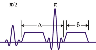
Figure 2. 2 Stejskal/Tanner diffusion preparation: Initial 90° RF pulse, followed by first diffusion lobe, 180° refocusing RF pulse, then second diffusion lobe. Leading edges of diffusion lobes are separated by ∆. Each lobe has duration δ
The theoretical curves were plotted versus the gradient parameter, $\text { bfactor, } \mathbf{b}^{\prime} \text { factor, } \overrightarrow{\mathbf{b}} \text { factor, Sfactor, } \mathbf{b}^{*}$ $\text { and } G_{z}$ for selected values of ∆, δ, $G_{z}$, β and µ Figure 2. As an example of the behavior expected, the decay of the normalized magnetization ($\frac{M_{x y}}{M_{0}}$), as given in Eq. (2), is plotted in Figure 3 versus $b_{\text {factor }}^{*} \text { where } b_{\text {factor }}^{*}=0 \text { to } 180 \mathrm{~s} / \mathrm{mm}^{2}$ and $b_{\text {factor }}^{*}=\left(\gamma \mathrm{G}_{\mathrm{z}} \delta\right)^{2}\left(\Delta-\frac{2 \beta-1}{2 \beta+1} \delta\right)$ for different values of $\mathrm{D}_{\beta}$ in the range from $\mathrm{D}_{\beta}=0.8333 \times 10^{-3} \mathrm{~mm}^{2} / \mathrm{s}$ (bottom curve) to $\mathrm{D}_{\beta}=3.333 \times 10^{-3} \mathrm{~mm}^{2} / \mathrm{s}$ in steps of 0.8333 $\times 10^{-3} \mathrm{~mm}^{2} / \mathrm{s}$ ($\Delta=40 \times 10^{-3} s$, µ = 5µm, β= 0.6, $\delta=1 \times 10^{-3} \mathrm{~s}$, γ= 42.58 MHz/T). We observed that as $\mathrm{D}_{\beta}$ increases the normalized magnetization curve change from heavy tailed decay to a straight line which strongly resembles the behavior recorded in restricted diffusion. In Figure 4 normalized magnetization $M_{x y} / M_{0} \text { is plotted versus } b_{\text {factor }}^{*}$ where 17=0 to 180 $s / m m^{2} \text { and } b_{\text {factor }}^{*}$ for different values of $\mu_{\beta}$ in the range from $\mu_{\beta}$ = 3.333µm (bottom curve) to $\mu_{\beta}$ = 16.6667µm in steps of 3.333µm (∆ = 40 $\times 10^{-3}$s, D = $1 \times 10^{-3} \mathrm{~mm}^{2} / \mathrm{s}, G_{\mathrm{z}}=0 \text { to } 1.5 \mathrm{~T} / \mathrm{m}, \delta=1 \times 10^{-3} \mathrm{~s}$, β=0.6, γ= 42.58 MHz/T). In Figure 5 normalized magnetization $M_{x y} / M_{0}$ is plotted versus $b_{\text {factor }}$ where $b_{\text {factor }}$ = 0 to 1800 $s / m m^{2} \text { and } b_{\text {factor }}=\left(\gamma \mathrm{G}_{\mathrm{z}} \delta\right)^{2} \Delta \text { and } \Delta \gg \delta$ for different values of $\mathrm{D}_{\beta} \text { in the range from } \mathrm{D}_{\beta}=0.8333 \times 10^{-3} \mathrm{~mm}^{2} / \mathrm{s}$ (bottom curve) to $\mathrm{D}_{\beta}=3.333 \times 10^{-3} \mathrm{~mm}^{2} / \mathrm{s}$ in steps of $0.8333 \times 10^{-3} \mathrm{~mm}^{2} / \mathrm{s}$ (∆ = 40 $\times 10^{-3} s$, µ = 5µm, β= 0.6, $\delta=1 \times 10^{-3} \mathrm{~s}$, γ= 42.58 MHz/T). In Figure 6 normalized magnetization $M_{x y} / M_{0} \text { is plotted versus } b_{\text {factor }}$ where $b_{\text {factor }}=0 \text { to } 1800 \mathrm{~s} / \mathrm{mm}^{2} \text { and } b_{\text {factor }}$ and $\Delta \gg \delta$ for different values of $\mu_{\beta}$ in the range from $\mu_{\beta}=3.333 \mu \mathrm{m}$ (bottom curve) to $\mu_{\beta}$ = 16.6667µm in steps of 3.333µm (∆ = 40 $\times 10^{-3}$s, $\mathrm{D}=1 \times 10^{-3} \mathrm{~mm}^{2} / \mathrm{s}, G_{\mathrm{z}}=0 \text { to } 1.5 \mathrm{~T} / \mathrm{m}, \delta=1 \times 10^{-3} \mathrm{~s}$, β=0.6, γ= 42.58 MHz/T).
In this part we observe that as the value of $\mu_{\beta}$ increases the contribution of restricted diffusion increase for a fixed value of β. We can see this behavior when Eq. (2) is written either in terms of a single exponential decay, $e^{-b D_{a p I}}$, where: $\text {DapI}=\frac{D}{\left(\left(\gamma G_{z} \delta\right) \mu\right)^{2(1-\beta)}}$; or when Eq. (2) is written as a stretched exponential, $e^{-\left(b D_{F}\right)^{\beta}}, \text { where } D_{F}^{\beta}=D\left(\Delta / \mu^{2}\right)^{1-\beta}$. Also when $\mu=\sqrt{D \Delta}$ it can be shown that the exponential form is ‘‘stretched exponential’’ result, $e^{-(b D)^{\beta}}$ considered by Bennett [12, 17-20]. In Figure 5 when $\mu_{\beta}=$ = 7.07/0.6 µm, we observed a decrease in the apparent diffusion coefficient $\mathrm{D}_{\beta}$ as the values of β decrease and $\mu_{\beta}$ increase.
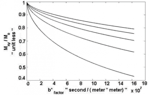
Figure 3. Stretched exponential model curves plot:
$\mathrm{M}_{\mathrm{xy}} / \mathrm{M}_{0}$ Versus $\mathrm{b}_{\text {factor }}^{*}$ where $\mathrm{b}_{\text {factor }}^{*}=0$ to $18 \times 10^{7} \mathrm{~s} / \mathrm{m}^{2}$ and $\mathrm{b}_{\text {factor }}^{*}=\left(\gamma \mathrm{G}_{\mathrm{z}} \delta\right)^{2}\left(\Delta-\frac{2 \beta-1}{2 \beta+1} \delta\right)$ for different values of $\mathrm{D}_{\beta}$ in
the range from $D_{\beta}=0.8333 \times 10^{-3} \mathrm{~mm}^{2} / \mathrm{s}$ (bottom curve) to $\mathrm{D}_{\beta}=3.333 \times 10^{-3} \mathrm{~mm}^{2} / \mathrm{s}$ in steps of $0.8333 \times 10^{-3} \mathrm{~mm}^{2} / \mathrm{s}(\Delta=$
$
\left.40 \times 10^{-3} \mathrm{~s}, \mu=5 \mu \mathrm{m}, \beta=0.6, \delta=1 \times 10^{-3} \mathrm{~s}, \gamma=42.58 \mathrm{MHz} / \mathrm{T}\right)
$
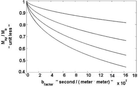
Figure 4. Stretched exponential model curves plot:
$\mathrm{M}_{\mathrm{xy}} / \mathrm{M}_{0}$ versus $\mathrm{b}_{\text {factor }}^{*}$ where $\mathrm{b}_{\text {factor }}^{*}=0$ to $18 \times 10^{7} \mathrm{~s} / \mathrm{m}^{2}$ and $\mathrm{b}_{\text {factor }}^{*}=\left(\gamma \mathrm{G}_{\mathrm{z}} \delta\right)^{2}\left(\Delta-\frac{2 \beta-1}{2 \beta+1} \delta\right)$ for different values of $\mu_{\beta}$ in
the range from $\mu_{\beta}=3.333 \mu \mathrm{m}$ (bottom curve) to $\mu_{\beta}=16.6667 \mu \mathrm{m}$ in steps of $3.333 \mu \mathrm{m}\left(\Delta=40 \times 10^{-3} \mathrm{~s}, \mathrm{D}=1 \times 10^{-3} \mathrm{~mm}^{2} / \mathrm{s},\right.$
$
\mathrm{G}_{\mathrm{z}}=0 \text { to } \left.1.5 \mathrm{~T} / \mathrm{m}, \delta=1 \times 10^{-3} \mathrm{~s}, \beta=0.6, \gamma=42.58 \mathrm{MHz} / \mathrm{T}\right)
$
Figure 5. Stretched exponential model curves plot:
$\mathrm{M}_{\mathrm{xy}} / \mathrm{M}_{0}$ Versus $\mathrm{b}_{\text {factor }}$ where $\mathrm{b}_{\text {factor }}=0$ to $18 \times 10^{8} \mathrm{~s} / \mathrm{m}^{2}$ and $\mathrm{b}_{\text {factor }}=\left(\gamma \mathrm{G}_{\mathrm{z}} \delta\right)^{2} \Delta$ and $\Delta \gg \delta$ for different values of $\mathrm{D}_{\beta}$ in
the range from $D_{\beta}=0.8333 \times 10^{-3} \mathrm{~mm}^{2} / \mathrm{s}$ (bottom curve) to $\mathrm{D}_{\beta}=3.333 \times 10^{-3} \mathrm{~mm}^{2} / \mathrm{s}$ in steps of $0.8333 \times 10^{-3} \mathrm{~mm}^{2} / \mathrm{s}$ ( $\Delta=$
$
\left.40 \times 10^{-3} \mathrm{~s}, \mu=5 \mu \mathrm{m}, \beta=0.6, \delta=1 \times 10^{-3} \mathrm{~s}, \gamma=42.58 \mathrm{MHz} / \mathrm{T}\right)
$
Figure 6. Stretched exponential model curves plot:
$\mathrm{M}_{\mathrm{xy}} / \mathrm{M}_{0}$ versus $\mathrm{b}_{\text {factor }}$ where $\mathrm{b}_{\text {factor }}=0$ to $18 \times 10^{7} \mathrm{~s} / \mathrm{m}^{2}$ and $\mathrm{b}_{\text {factor }}=\left(\gamma \mathrm{G}_{\mathrm{z}} \delta\right)^{2} \Delta$ and $\Delta \gg \delta$ for different values of $\mu_{\beta}$ in the range from $\mu_{\beta}=3.333 \mu \mathrm{m}$ (bottom curve) to $\mu_{\beta}=16.6667 \mu \mathrm{m}$ in steps of $3.333 \mu \mathrm{m}$
$\left(\Delta=40 \times 10^{-3} \mathrm{~s}, \mathrm{D}=1 \times 10^{-3} \mathrm{~mm}^{2} / \mathrm{s}, \mathrm{G}_{\mathrm{z}}=0 \text { to } 1.5 \mathrm{~T} / \mathrm{m}, \delta=1 \times 10^{-3} \mathrm{~s}, \beta=0.6, \gamma=42.58 \mathrm{MHz} / \mathrm{T}\right)$
Figure 7. Stretched Exponential Model Curves Plot:
$\mathrm{M}_{\mathrm{xy}} / \mathrm{M}_{0}$ Versus $\mathrm{G}_{\mathrm{z}}$ where $\mathrm{G}_{\mathrm{z}}=0$ to $1.5 \mathrm{~T} / \mathrm{m}$ for different values of $\mathrm{D}_{\beta}$ in the range $\mathrm{from} \mathrm{D}_{\beta}=0.8333 \times 10^{-3} \mathrm{~mm}^{2} / \mathrm{s}$
(bottom curve) to $D_{\beta}=3.333 \times 10^{-3} \mathrm{~mm}^{2} / \mathrm{s}$ in steps of $0.8333 \times 10^{-3} \mathrm{~mm}^{2} / \mathrm{s}$
$
\left(\Delta=40 \times 10^{-3} \mathrm{~s}, \mu=5 \mu \mathrm{m}, \beta=0.6, \delta=1 \times 10^{-3} \mathrm{~s}, \gamma=42.58 \mathrm{MHz} / \mathrm{T}\right)
$
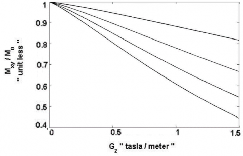
Figure 8. Stretched exponential model curves plot:
$\mathrm{M}_{\mathrm{xy}} / \mathrm{M}_{0}$ Versus $\mathrm{G}_{\mathrm{z}}$ where $\mathrm{G}_{\mathrm{z}}=0$ to $1.5 \mathrm{~T} / \mathrm{m}$ for different
values of $\mu$ in the range from $\mu_{\beta}=3.333 \mu \mathrm{m}$ (bottom curve) to $\mu_{\beta}=16.6667 \mu \mathrm{m}$ in steps of $3.333 \mu \mathrm{m}\left(\Delta=40 \times 10^{-3} \mathrm{~s}, \mathrm{D}=\right.$
$
\begin{aligned}
1 \times 10^{-3} \mathrm{~mm}^{2} / \mathrm{s}, \mathrm{G}_{\mathrm{z}} &=0 \text { to } 1.5 \mathrm{~T} / \mathrm{m}, \delta=1 \times 10^{-3} \mathrm{~s}, \beta=0.6 \\
\gamma &=42.58 \mathrm{MHz} / \mathrm{T})
\end{aligned}
$
Figure 9. Stretched exponential model curves plot:
$\mathrm{M}_{\mathrm{xy}} / \mathrm{M}_{0} \text { Versus } \overline{\mathrm{b}} \text { factor where } \overline{\mathrm{b}} \text { factor }=0 \text { to } 2.5 \times 10^{8} \mathrm{~s} / \mathrm{m}^{2} \text { and } \overline{\mathrm{b}} \text { factor }=\frac{1}{\beta \mu_{\mathrm{\beta}}^{2}}\left(\gamma \mathrm{G}_{\mathrm{z}} \delta \beta \mu_{\beta}\right)^{2 \beta}\left(\Delta-\frac{2 \beta-1}{2 \beta+1} \delta\right) \text { for different }$
$\text { values of } D_{\beta} \text { in the range from } D_{\beta}=0.8333 \times 10^{-3} \mathrm{~mm}^{2} / \mathrm{s} \text { (bottom curve) to } \mathrm{D}_{\beta}=3.333 \times 10^{-3} \mathrm{~mm}^{2} / \mathrm{s} \text { in steps of }$
$0.8333 \times 10^{-3} \mathrm{~mm}^{2} / \mathrm{s}\left(\Delta=40 \times 10^{-3} \mathrm{~s}, \mu=5 \mu \mathrm{m}, \beta=0.6, \delta=1 \times 10^{-3} \mathrm{~s}, \gamma=42.58 \mathrm{MHz} / \mathrm{T}\right)$
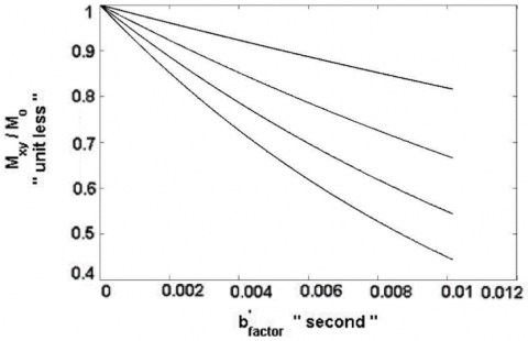
Figure 10. Stretched exponential model curves plot:
$\mathrm{M}_{\mathrm{xy}} / \mathrm{M}_{0}$ Versus $\mathrm{b}_{\text {factor }}^{\prime}$ where $\mathrm{b}_{\text {factor }}^{\prime}=0$ to 0.01 second and $\mathrm{b}_{\text {factor }}^{\prime}=\left(\gamma \mathrm{G}_{\mathrm{z}} \delta \beta \mu_{\beta}\right)^{2 \beta}\left(\Delta-\frac{2 \beta-1}{2 \beta+1} \delta\right)$ for different values of $\mathrm{D}_{\beta}$ in the
range from $\mathrm{D}_{\beta}=0.8333 \times 10^{-3} \mathrm{~mm}^{2} / \mathrm{s}$ (bottom curve) to $\mathrm{D}_{\beta}=3.333 \times 10^{-3} \mathrm{~mm}^{2} / \mathrm{s}$ in steps of $0.8333 \times 10^{-3} \mathrm{~mm}^{2} / \mathrm{s}$ ( $\Delta=$
$
\left.40 \times 10^{-3} \mathrm{~s}, \mu=5 \mu \mathrm{m}, \beta=0.6, \delta=1 \times 10^{-3} \mathrm{~s}, \gamma=42.58 \mathrm{MHz} / \mathrm{T}\right)
$
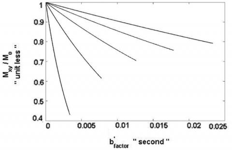
Figure 11. Stretched exponential model curves plot:
$\mathrm{M}_{\mathrm{xy}} / \mathrm{M}_{0}$ versus $\mathrm{b}_{\text {factor }}^{\prime}$ where $\mathrm{b}_{\text {factor }}^{\prime}=0$ to 0.025 second and $\mathrm{b}_{\text {factor }}^{\prime}=\left(\gamma \mathrm{G}_{\mathrm{z}} \delta \beta \mu_{\beta}\right)^{2 \beta}\left(\Delta-\frac{2 \beta-1}{2 \beta+1} \delta\right)$ for different values of $\mu_{\beta}$ in
the range from $\mu_{\beta}=3.333 \mu \mathrm{m}$ (bottom curve) to $\mu_{\beta}=16.6667 \mu \mathrm{m}$ in steps of $3.333 \mu \mathrm{m}\left(\Delta=40 \times 10^{-3} \mathrm{~s}, \mathrm{D}=1 \times 10^{-3} \mathrm{~mm}^{2} / \mathrm{s},\right.$
$
\mathrm{G}_{\mathrm{z}}=0 \text { to } \left.1.5 \mathrm{~T} / \mathrm{m}, \delta=1 \times 10^{-3} \mathrm{~s}, \beta=0.6, \gamma=42.58 \mathrm{MHz} / \mathrm{T}\right)
$
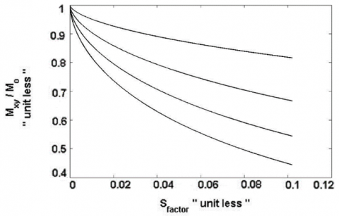
Figure 12. Stretched exponential model curves plot:
$\mathrm{M}_{\mathrm{xy}} / \mathrm{M}_{0}$ Versus $S_{\text {factor }}$ where $S_{\text {factor }}=0$ to 0.1 and $S_{\text {factor }}=\left(\gamma \mathrm{G}_{\mathrm{z}} \delta \beta \mu_{\beta}\right)^{2}$ for different values of $\mathrm{D}_{\beta}$ in the range from $\mathrm{D}_{\beta}=0.8333 \times 10^{-3} \mathrm{~mm}^{2} / \mathrm{s}$ (bottom curve) to $\mathrm{D}_{\beta}=3.333 \times 10^{-3} \mathrm{~mm}^{2} / \mathrm{s}$ in steps of $0.8333 \times 10^{-3} \mathrm{~mm}^{2} / \mathrm{s}$
$
\left(\Delta=40 \times 10^{-3} \mathrm{~s}, \mu=5 \mu \mathrm{m}, \beta=0.6, \delta=1 \times 10^{-3} \mathrm{~s}, \gamma=42.58 \mathrm{MHz} / \mathrm{T}\right)
$
Figure 13. Stretched exponential model curves plot:
$\mathrm{M}_{\mathrm{xy}} / \mathrm{M}_{0}$ versus $\mathrm{S}_{\text {factor }}$ where $\mathrm{S}_{\text {factor }}=0$ to 0.45 and $\mathrm{S}_{\text {factor }}=\left(\gamma \mathrm{G}_{\mathrm{z}} \delta \beta \mu_{\beta}\right)^{2}$ for different values of $\mu_{\beta}$ in the range from $\mu_{\beta}=3.333 \mu \mathrm{m}$ (bottom curve) to $\mu_{\beta}=16.6667 \mu \mathrm{m}$ in steps of $3.333 \mu \mathrm{m}$
$
\left(\Delta=40 \times 10^{-3} \mathrm{~s}, \mathrm{D}=1 \times 10^{-3} \mathrm{~mm}^{2} / \mathrm{s}, \mathrm{G}_{\mathrm{z}}=0 \text { to } 1.5 \mathrm{~T} / \mathrm{m}, \delta=1 \times 10^{-3} \mathrm{~s}, \beta=0.6, \gamma=42.58 \mathrm{MHz} / \mathrm{T}\right)
$
Figure 14. Stretched exponential model curves plot:
$\mathrm{M}_{\mathrm{xy}} / \mathrm{M}_{0}$ Versus $\overline{\mathrm{b}}$ factor where $\overline{\mathrm{b}}$ factor $=0$ to $2.5 \times 10^{8}$
$\mathrm{s} / \mathrm{m}^{2}$ and $\overline{\mathrm{b}}$ factor $=\frac{1}{\beta \mu_{\beta}^{2}}\left(\gamma \mathrm{G}_{\mathrm{z}} \delta \beta \mu_{\beta}\right)^{2 \beta}\left(\Delta-\frac{2 \beta-1}{2 \beta+1} \delta\right)$ for
different values of $\beta$ in the range from $\beta=0.6$ (bottom curve) to $\beta=0.9$ in steps of $0.1\left(\mathrm{D}=1^{*} 10^{-3} \mathrm{~mm}^{2} / \mathrm{s}, \mu=5 \mu \mathrm{m}, \mathrm{G}_{\mathrm{z}}=\right.$
0 to $1.5 \mathrm{~T} / \mathrm{m}, \delta=1 \times 10^{-3} \mathrm{~s}, \Delta=40 \times 10^{-3} \mathrm{~s}, \gamma=42.58$
$\mathrm{MHz} / \mathrm{T})$
In Figure 7 normalized magnetization $M_{x y} / M_{0}$ is plotted versus $G_{z} \text { where } G_{z}=0 \text { to } 1.5 \mathrm{~T} / \mathrm{m} \text { for different values of } D_{\beta}$ in the range from $\mathrm{D}_{\beta}=0.8333 \times 10^{-3} \mathrm{~mm}^{2} / \mathrm{s}$ (bottom curve) to $\mathrm{D}_{\beta}$ = 3.333 $10^{-3} \mathrm{~mm}^{2}$/s in steps of 0.8333 $10^{-3} \mathrm{~mm}^{2}$/s (∆ = 40 $\times 10^{-3} s$, µ = 5µm, β= 0.6, δ=1 $\times 10^{-3} s$, γ= 42.58 MHz/T). In Figure 8 normalized magnetization $M_{x y} / M_{0}$ is plotted versus $G_{z} \text { where } G_{z}$ = 0 to 1.5 T/m for different values of $\mu_{\beta}$ in the range from $\mu_{\beta}$ = 3.333µm (bottom curve) to $\mu_{\beta}$ = 16.6667µm in steps of 3.333µm (∆ = 40 $\times 10^{-3}$s, D = $1 \times 10^{-3} \mathrm{~mm}^{2} / \mathrm{s}, G_{\mathrm{z}}=0 \text { to } 1.5 \mathrm{~T} / \mathrm{m}, \delta=1 \times 10^{-3} \mathrm{~s}$, β=0.6, γ= 42.58 MHz/T). In Figure 9 normalized magnetization $M_{x y} / M_{0}$ is plotted versus $\overline{\mathrm{b}}$ factor where $\overline{\mathrm{b}}$ factor $=0$ to $250 \mathrm{~s} / \mathrm{mm}^{2}$ and $\overline{\mathrm{b}}$ factor $=\frac{1}{\beta \mu_{\beta}^{2}}\left(\gamma \mathrm{G}_{\mathrm{z}} \delta \beta \mu_{\beta}\right)^{2 \beta}\left(\Delta-\frac{2 \beta-1}{2 \beta+1} \delta\right) \quad$ for $\quad$ different values of $\mathrm{D}_{\beta}$ in the range from $\mathrm{D}_{\beta}=0.8333 \times 10^{-3} \mathrm{~mm}^{2} / \mathrm{s}$ (bottom curve) to $\mathrm{D}_{\beta}=3.333 \times 10^{-3} \mathrm{~mm}^{2} / \mathrm{s}$ in steps of $0.8333 \times 10^{-3} \mathrm{~mm}^{2} / \mathrm{s}\left(\Delta=40 \times 10^{-3} \mathrm{~s}, \mu=5 \mu \mathrm{m}, \beta=0.6\right.$ $\left.\delta=1 \times 10^{-3} \mathrm{~s}, \gamma=42.58 \mathrm{MHz} / \mathrm{T}\right)$. In Figure 10 normalized magnetization $M_{x y} / M_{0}$ is plotted versus $\mathrm{b}_{\text {factor}}^{\prime}$ where $\mathrm{b}_{\text {factor}}^{\prime}=0$ to 0.01 second and $\mathrm{b}_{\text {factor}}^{\prime}=$ $\left(\gamma \mathrm{G}_{\mathrm{z}} \delta \beta \mu_{\beta}\right)^{2 \beta}\left(\Delta-\frac{2 \beta-1}{2 \beta+1} \delta\right)$ for different values of $\mathrm{D}_{\beta}$ in the range from $D_{\beta}=0.8333 \times 10^{-3} \mathrm{~mm}^{2} / \mathrm{s}$ (bottom curve) to $\mathrm{D}_{\beta}=$ $3.333 \times 10^{-3} \mathrm{~mm}^{2} / \mathrm{s}$ in steps of $0.8333 \times 10^{-3} \mathrm{~mm}^{2} / \mathrm{s}(\Delta=$ $\left.40 \times 10^{-3} s, \mu=5 \mu \mathrm{m}, \beta=0.6, \delta=1 \times 10^{-3} \mathrm{~s}, \gamma=42.58 \mathrm{MHz} / \mathrm{T}\right)$. In Figure 11 stretched exponential model curves plot, $\mathbf{M}_{\mathrm{xy}} / \mathrm{M}_{0}$ versus $\mathbf{b}_{\mathrm{factor}}^{\prime}$ where $\mathbf{b}_{\mathrm{factor}}^{\prime}=0$ to $0.025 \mathrm{~second}$ and $\mathbf{b}_{\text {factor }}^{\prime}=\left(\gamma G_{z} \delta \beta \mu_{\beta}\right)^{2 \beta}\left(\Delta-\frac{2 \beta-1}{2 \beta+1} \delta\right)$ for different values of $\mu_{\beta}$ in the range from $\mu_{\beta}=3.333 \mu \mathrm{m}$ (bottom curve) to $\mu_{\beta}=$ $16.6667 \mu \mathrm{m}$ in steps of $3.333 \mu \mathrm{m}\left(\Delta=40 \times 10^{-3} \mathrm{~s}, \mathrm{D}=\right.$ $1 \times \mathbf{1 0}^{-3} \mathbf{m m}^{2} / \mathbf{s}, \mathbf{G}_{\mathbf{z}}=\mathbf{0}$ to $\mathbf{1 . 5} \mathrm{T} / \mathrm{m}, \delta=1 \times \mathbf{1 0}^{-3} \mathrm{~s}, \beta=0.6$ $\gamma=42.58 \mathrm{MHz} / \mathrm{T})$.
In Figure 13 normalized magnetization $M_{x y} / M_{0}$ is plotted versus $\mathrm{b}_{\text {factor}}^{\prime}$ where $\mathrm{b}_{\text {factor}}^{\prime}=0$ to 0.025 second for different values of $\mu_{\beta}$ in the range from $\mu_{\beta}=3.333 \mu \mathrm{m}$ (bottom curve) to $\mu_{\beta}=16.6667 \mu \mathrm{m}$ in steps of $3.333 \mu \mathrm{m}\left(\Delta=40 \times 10^{-3} \mathrm{~s}, \mathrm{D}=\right.$ $1 \times 10^{-3} \mathrm{~mm}^{2} / \mathrm{s}, G_{z}=0$ to $1.5 \mathrm{~T} / \mathrm{m}, \delta=1 \times 10^{-3} \mathrm{~s}, \beta=0.6, \gamma=$ $\begin{array}{lllll}42.58 & \text { MHz/T). } & \text { In Figure } & 12 & \text { normalized } & \text { magnetization }\end{array}$ $M_{x y} / M_{0}$ is plotted versus $S_{\text {factor}}$ where $S_{\text {factor}}=0$ to 0.1 and $S_{\text {factor}}=\left(\gamma G_{z} \delta \beta \mu_{\beta}\right)^{2}$ for different values of $D_{\beta}$ in the range from $\mathrm{D}_{\beta}=0.8333 \times 10^{-3} \mathrm{~mm}^{2} / \mathrm{s}$ (bottom curve) to $\mathrm{D}_{\beta}=$ $3.333 \times 10^{-3} \mathrm{~mm}^{2} / \mathrm{s}$ in steps of $0.8333 \times 10^{-3} \mathrm{~mm}^{2} / \mathrm{s}(\Delta=$ $\left.40 \times 10^{-3} s, \mu=5 \mu \mathrm{m}, \beta=0.6, \delta=1 \times 10^{-3} \mathrm{~s}, \gamma=42.58 \mathrm{MHz} / \mathrm{T}\right)$ In Figure 13 normalized magnetization $M_{x y} / M_{0}$ is plotted versus Sfactar where $S_{\text {factar }}=0$ to 0.45 for different values of $\mu_{\beta}$ in the range from $\mu_{\beta}=3.333 \mu \mathrm{m}$ (bottom curve) to $\mu_{\beta}=$ 16.6667\mum in steps of $3.333 \mu \mathrm{m}\left(\Delta=40 \times 10^{-3} \mathrm{~s}, \mathrm{D}=\right.$ $1 \times 10^{-3} \mathrm{~mm}^{2} / \mathrm{s}, G_{z}=0$ to $1.5 \mathrm{~T} / \mathrm{m}, \delta=1 \times 10^{-3} \mathrm{~s}, \beta=0.6, \gamma=$ $\begin{array}{llllll}42.58 & \text { MHz/T). } & \text { We observed that the } & \text { normalized }\end{array}$ magnetization curve change from heavy tailed decay to a straight line as $\mathrm{D}_{\beta}$ increases and $\mu_{\beta}$ increases. Which strongly resembles the behavior of restricted diffusion.
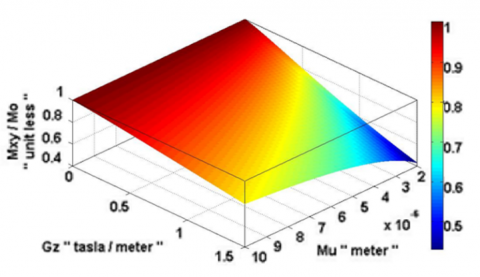
Figure 15. Stretched exponential model surface plot:
$\mathrm{M}_{\mathrm{xy}} / \mathrm{M}_{\mathrm{o}} \text { Versus } \mathrm{G}_{\mathrm{z}} \text { where } \mathrm{G}_{\mathrm{z}}=0 \text { to } 1.5 \mathrm{~T} / \mathrm{m} \text { and } \mu \text { where } \mu=2 \text { to } 10 \mu \mathrm{m}$.
$\left(\mathrm{D}=1 \times 10^{-3} \mathrm{~mm}^{2} / \mathrm{s}, \beta=0.6, \delta=1 \times 10^{-3} \mathrm{~s}, \Delta=40 \times 10^{-3} \mathrm{~s}, \gamma=42.58 \mathrm{MHz} / \mathrm{T}\right)$
Figure 16. Stretched exponential model surface plot:
$\mathrm{M}_{\mathrm{xy}} / \mathrm{M}_{\mathrm{o}} \text { Versus } \beta \text { where } \beta=0.5 \text { to } 1 \text { and } \mu \text { where } \mu=2 \text { to } 10 \mu \mathrm{m}$.
$\left(\mathrm{D}=1 \times 10^{-3} \mathrm{~mm}^{2} / \mathrm{s}, \mathrm{G}_{\mathrm{z}}=1.5 \mathrm{~T} / \mathrm{m}, \delta=1 \times 10^{-3} \mathrm{~s}, \Delta=40 \times 10^{-3} \mathrm{~s}, \gamma=42.58 \mathrm{MHz} / \mathrm{T}\right)$
Figure 17. Stretched exponential model surface plot:
$\begin{equation}\mathrm{M}_{\mathrm{xv}} / \mathrm{M}_{\mathrm{o}} \text { Versus } \mathrm{D} \text { where } \mathrm{D}=1 \times 10^{-3} \text {to } 10 \times 10^{-3} \mathrm{~mm}^{2} / \mathrm{s} \text { and } \mu \text { where } \mu=2 \text { to } 10 \mu \mathrm{m}\end{equation}$.
$\begin{equation}\left(\beta=0.6, \mathrm{G}_{\mathrm{z}}=1.5 \mathrm{~T} / \mathrm{m}, \delta=1 \times 10^{-3} \mathrm{~s}, \Delta=40 \times 10^{-3} \mathrm{~s}, \gamma=42.58 \mathrm{MHz} / \mathrm{T}\right)\end{equation}$
Figure 18. Stretched exponential model surface plot:
$\begin{equation}\mathrm{M}_{\mathrm{xy}} / \mathrm{M}_{\mathrm{o}} \text { Versus } \beta \text { where } \beta=0.5 \text { to } 1 \text { and } \mathrm{D} \text { where } \mathrm{D}=1 \times 10^{-3} \mathrm{to} 10 \times 10^{-3} \mathrm{~mm}^{2} / \mathrm{s}\end{equation}$.
$\begin{equation}\left(\mu=2 \times 10^{-6} \mathrm{~m}, \mathrm{G}_{\mathrm{z}}=1.5 \mathrm{~T} / \mathrm{m}, \delta=1 \times 10^{-3} \mathrm{~s}, \Delta=40 \times 10^{-3} \mathrm{~s}, \gamma=42.58 \mathrm{MHz} / \mathrm{T}\right)\end{equation}$
Figure 19. Stretched exponential model surface plot:
$\begin{equation}\mathrm{M}_{\mathrm{xy}} / \mathrm{M}_{\mathrm{o}} \text { Versus } \beta \text { where } \beta=0.5 \text { to } 1 \text { and } \Delta \text { where } \Delta=40 \times 10^{-3} \text {to } 400 \times 10^{-3} \mathrm{~s}\end{equation}$.
$\begin{equation}\left(\mu=2 \times 10^{-6} \mathrm{~m}, \mathrm{G}_{\mathrm{z}}=1.5 \mathrm{~T} / \mathrm{m}, \delta=1 \times 10^{-3} \mathrm{~s}, \mathrm{D}=1 \times 10^{-3} \mathrm{~mm}^{2} / \mathrm{s}, \gamma=42.58 \mathrm{MHz} / \mathrm{T}\right)\end{equation}$
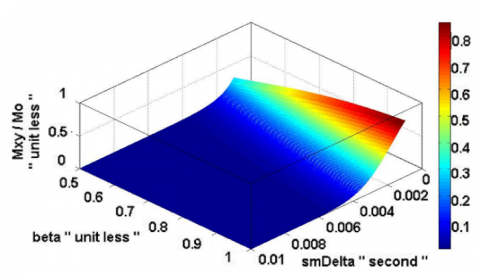
Figure 20. Stretched exponential model surface plot:
$\begin{equation}\mathrm{M}_{\mathrm{xy}} / \mathrm{M}_{\mathrm{o}} \text { Versus } \beta \text { where } \beta=0.5 \text { to } 1 \text { and } \delta \text { where } \delta=1 \times 10^{-3} \text {to } 10 \times 10^{-3} \mathrm{~s}\end{equation}$.
$\begin{equation}\left(\mu=2 \times 10^{-6} \mathrm{~m}, \mathrm{G}_{\mathrm{z}}=1.5 \mathrm{~T} / \mathrm{m}, \Delta=40 \times 10^{-3} \mathrm{~s}, \mathrm{D}=1 \times 10^{-3} \mathrm{~mm}^{2} / \mathrm{s}, \gamma=42.58 \mathrm{MHz} / \mathrm{T}\right)\end{equation}$
Figure 21. Stretched exponential model surface plot:
$\begin{equation}\mathrm{M}_{\mathrm{xy}} / \mathrm{M}_{\mathrm{o}} \text { Versus } \Delta \text { where } \Delta=40 \times 10^{-3} \text {to } 400 \times 10^{-3} \mathrm{~s} \text { and } \delta \text { where } \delta=1 \times 10^{-3} \text {to } 10 \times 10^{-3} \mathrm{~s}\end{equation}$.
$\begin{equation}\left(\mu=2 \times 10^{-6} \mathrm{~m}, \mathrm{G}_{\mathrm{z}}=1.5 \mathrm{~T} / \mathrm{m}, \beta=0.6, \mathrm{D}=1 \times 10^{-3} \mathrm{~mm}^{2} / \mathrm{s}, \gamma=42.58 \mathrm{MHz} / \mathrm{T}\right)\end{equation}$
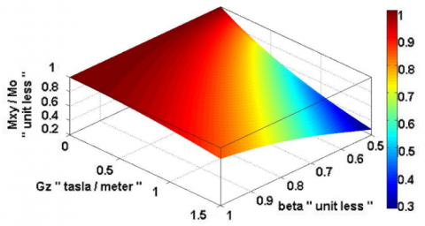
Figure 22. Stretched exponential model surface plot
$\mathrm{M}_{\mathrm{xy}} / \mathrm{M}_{\mathrm{o}} \text { Versus } \mathrm{G}_{\mathrm{z}} \text { where } \mathrm{G}_{\mathrm{z}}=0 \text { to } 1.5 \mathrm{~T} / \mathrm{m} \text { and } \beta \text { where } \beta=0.5 \text { to } 1.$
$\left(\mu=2 \times 10^{-6} \mathrm{~m}, \Delta=40 \times 10^{-3} \mathrm{~s}, \delta=1 \times 10^{-3} \mathrm{~s}, \mathrm{D}=1 \times 10^{-3} \mathrm{~mm}^{2} / \mathrm{s}, \gamma=42.58 \mathrm{MHz} / \mathrm{T}\right)$
Figure 23. Stretched exponential model surface plot:
$\mathrm{M}_{\mathrm{xV}} / \mathrm{M}_{\mathrm{o}} \text { Versus } \mathrm{G}_{\mathrm{z}} \text { where } \mathrm{G}_{\mathrm{z}}=0 \text { to } 1.5 \mathrm{~T} / \mathrm{m} \text { and } \Delta \text { where } \Delta=40 \times 10^{-3} \text {to } 40 \times 10^{-3} \mathrm{~s}$.
$\left(\mu=2 \times 10^{-6} \mathrm{~m}, \beta=0.6, \delta=1 \times 10^{-3} \mathrm{~s}, \mathrm{D}=1 \times 10^{-3} \mathrm{~mm}^{2} / \mathrm{s}, \gamma=42.58 \mathrm{MHz} / \mathrm{T}\right)$
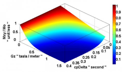
Figure 24. Stretched exponential model surface plot:
$\mathrm{M}_{\mathrm{xy}} / \mathrm{M}_{\mathrm{o}} \text { Versus } \mathrm{G}_{\mathrm{z}} \text { where } \mathrm{G}_{\mathrm{z}}=0 \text { to } 1.5 \mathrm{~T} / \mathrm{m} \text { and } \delta \text { where } \delta=1 \times 10^{-3} \text {to } 10 \times 10^{-3} \mathrm{~s}$.
$\left(\mu=2 \times 10^{-6} \mathrm{~m}, \beta=0.6, \Delta=40 \times 10^{-3} \mathrm{~s}, \mathrm{D}=1 \times 10^{-3} \mathrm{~mm}^{2} / \mathrm{s}, \gamma=42.58 \mathrm{MHz} / \mathrm{T}\right)$
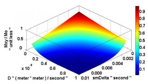
Figure 25. Stretched exponential model surface plot:
$\mathrm{M}_{\mathrm{xy}} / \mathrm{M}_{\mathrm{o}} \text { Versus } \mathrm{G}_{\mathrm{z}} \text { where } \mathrm{G}_{\mathrm{z}}=0 \text { to } 1.5 \mathrm{~T} / \mathrm{m} \text { and } \mathrm{D} \text { where } \mathrm{D}=1 \times 10^{-3} \text {to } 10 \times 10^{-3} \mathrm{~mm}^{2} / \mathrm{s}$.
$\left(\mu=2 \times 10^{-6} \mathrm{~m}, \beta=0.6, \Delta=40 \times 10^{-3} \mathrm{~s}, \delta=1 \times 10^{-3} \mathrm{~s}, \gamma=42.58 \mathrm{MHz} / \mathrm{T}\right)$
Figure 26. Stretched exponential model surface plot:
$\mathrm{M}_{\mathrm{xy}} / \mathrm{M}_{\mathrm{o}} \text { Versus } \delta \text { where } \delta=1 \times 10^{-3} \text {to } 10 \times 10^{-3} \mathrm{~s} \text { and } \mathrm{D} \text { where } \mathrm{D}=1 \times 10^{-3} \text {to } 10 \times 10^{-3} \mathrm{~mm}^{2} / \mathrm{s}$.
$\left(\mu=2 \times 10^{-6} \mathrm{~m}, \beta=0.6, \Delta=40 \times 10^{-3} \mathrm{~s}, \mathrm{G}_{\mathrm{z}}=1.5 \mathrm{~T} / \mathrm{m}, \gamma=42.58 \mathrm{MHz} / \mathrm{T}\right)$
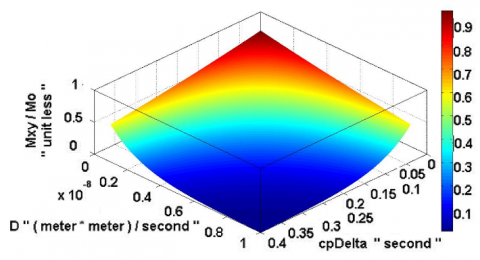
Figure 27. Stretched exponential model surface plot:
$\mathrm{M}_{\mathrm{xv}} / \mathrm{M}_{\mathrm{o}} \text { Versus } \delta \text { where } \Delta=40 \times 10^{-3} \text {to } 400 \times 10^{-3} \mathrm{~s} \text { and } \mathrm{D} \text { where } \mathrm{D}=1 \times 10^{-3} \text {to } 10 \times 10^{-3} \mathrm{~mm}^{2} / \mathrm{s}$.
$\left(\mu=2 \times 10^{-6} \mathrm{~m}, \beta=0.6, \delta=1 \times 10^{-3} \mathrm{~s}, \mathrm{G}_{\mathrm{z}}=1.5 \mathrm{~T} / \mathrm{m}, \gamma=42.58 \mathrm{MHz} / \mathrm{T}\right)$
Figure 28. Stretched exponential model surface plot:
$\mathrm{M}_{\mathrm{xy}} / \mathrm{M}_{\mathrm{o}} \text { Versus } \delta \text { where } \delta=1 \times 10^{-3} \text {to } 10 \times 10^{-3} \mathrm{~s} \text { and } \mu \text { where } \mu=2 \text { to } 10 \mu \mathrm{m}$.
$\left(\mathrm{D}=1 \times 10^{-3} \mathrm{~mm}^{2} / \mathrm{s}, \beta=0.6, \Delta=40 \times 10^{-3} \mathrm{~s}, \mathrm{G}_{\mathrm{z}}=1.5 \mathrm{~T} / \mathrm{m}, \gamma=42.58 \mathrm{MHz} / \mathrm{T}\right)$
Figure 29. Stretched exponential model surface plot:
$\mathrm{M}_{\mathrm{xy}} / \mathrm{M}_{\mathrm{o}} \text { Versus } \Delta \text { where } \Delta=40 \times 10^{-3} \text {to } 400 \times 10^{-3} \mathrm{~s} \text { and } \mu \text { where } \mu=2 \text { to } 10 \mu \mathrm{m}$.
$\left(\mathrm{D}=1 \times 10^{-3} \mathrm{~mm}^{2} / \mathrm{s}, \beta=0.6, \delta=1 \times 10^{-3} \mathrm{~s}, \mathrm{G}_{\mathrm{z}}=1.5 \mathrm{~T} / \mathrm{m}, \gamma=42.58 \mathrm{MHz} / \mathrm{T}\right)$
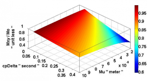
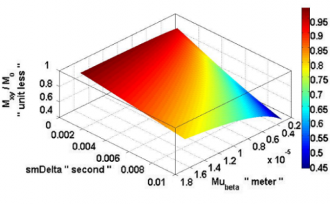
Figure 30. Stretched exponential model surface plot:
$\mathrm{M}_{\mathrm{xy}} / \mathrm{M}_{\mathrm{e}} \text { Versus } \mathrm{G}_{\mathrm{z}} \text { where } \mathrm{G}_{\mathrm{z}}=0 \text { to } 1.5 \mathrm{~T} / \mathrm{m} \text { and } \mu_{\beta} \text { where } \mu_{\mathrm{B}}=0.333 \times 10^{-5} \text {to } 1.67 \times 10^{-5} \mathrm{~m}$.
$\left(\mathrm{D}=1 \times 10^{-3} \mathrm{~mm}^{2} / \mathrm{s}, \beta=0.6, \delta=1 \times 10^{-3} \mathrm{~s}, \Delta=40 \times 10^{-3} \mathrm{~s}, \gamma=42.58 \mathrm{MHz} / \mathrm{T}\right)$
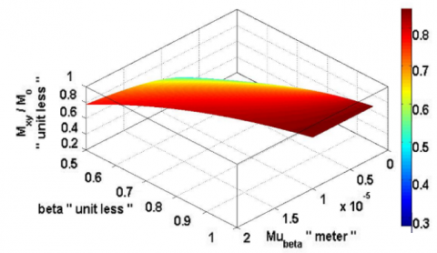
Figure 31. Stretched exponential model surface plot:
$\mathrm{M}_{\mathrm{xy}} / \mathrm{M}_{\mathrm{o}} \text { Versus } \beta \text { where } \beta=0.5 \text { to } 1 \text { and } \mu_{\beta} \text { where } \mu_{\beta}=0.333 \times 10^{-5} \text {to } 1.67 \times 10^{-5} \mathrm{~m}$.
$\left(\mathrm{D}=1 \times 10^{-3} \mathrm{~mm}^{2} / \mathrm{s}, \mathrm{G}_{\mathrm{z}}=1.5 \mathrm{~T} / \mathrm{m}, \delta=1 \times 10^{-3} \mathrm{~s}, \Delta=40 \times 10^{-3} \mathrm{~s}, \gamma=42.58 \mathrm{MHz} / \mathrm{T}\right)$
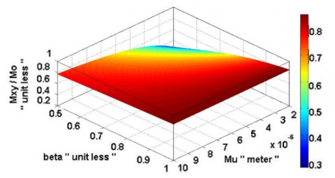
Figure 32. Stretched exponential model surface plot:
$\mathrm{M}_{\mathrm{xy}} / \mathrm{M}_{\mathrm{o}} \text { Versus } \mathrm{D}_{\beta} \text { where } \mathrm{D}_{\beta}=1.7 \times 10^{-3} \text {to } 16.7 \times 10^{-3} \mathrm{~mm}^{2} / \mathrm{s}, \text { and } \mu_{\mathrm{\beta}} \text { where } \mu_{\beta}=3.33 \times 10^{-5} \text {to } 1.67 \times 10^{-5} \mathrm{~m}$.
$\left(\beta=0.6, \mathrm{G}_{\mathrm{z}}=1.5 \mathrm{~T} / \mathrm{m}, \delta=1 \times 10^{-3} \mathrm{~s}, \Delta=40 \times 10^{-3} \mathrm{~s}, \gamma=42.58 \mathrm{MHz} / \mathrm{T}\right)$
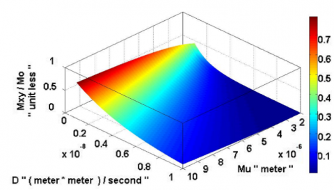
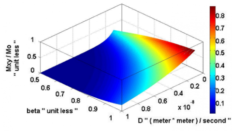
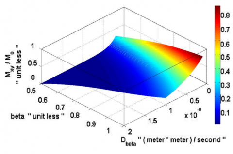
Figure 33. Stretched exponential model surface plot:
$\mathrm{M}_{\mathrm{xy}} / \mathrm{M}_{\mathrm{o}} \text { Versus } \mathrm{D}_{\beta} \text { where } \mathrm{D}_{\beta}=1.7 \times 10^{-3} \text {to } 16.7 \times 10^{-3} \mathrm{~mm}^{2} / \mathrm{s}, \text { and } \beta \text { where } \beta=0.5 \text { to } 1$.
$\left(\mu=2 \mu \mathrm{m}, \mathrm{G}_{\mathrm{z}}=1.5 \mathrm{~T} / \mathrm{m}, \delta=1 \times 10^{-3} \mathrm{~s}, \Delta=40 \times 10^{-3} \mathrm{~s}, \gamma=42.58 \mathrm{MHz} / \mathrm{T}\right)$
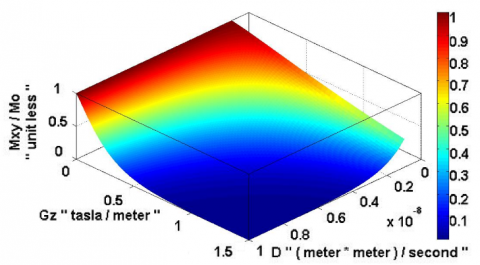
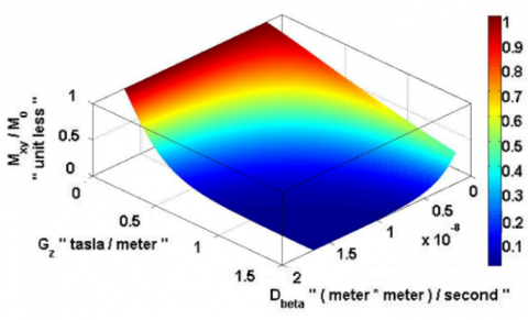
Figure 34. Stretched exponential model surface plot:
$\mathrm{M}_{\mathrm{xy}} / \mathrm{M}_{\mathrm{o}} \text { Versus } \mathrm{D}_{\beta} \text { where } \mathrm{D}_{\beta}=1.7 \times 10^{-3} \text {to } 16.7 \times 10^{-3} \mathrm{~mm}^{2} / \mathrm{s}, \text { and } \mathrm{G}_{\mathrm{z}} \text { where } \mathrm{G}_{\mathrm{z}}=0 \text { to } 1.5 \mathrm{~T} / \mathrm{m}$.
$\left(\mu=2 \mu \mathrm{m}, \beta=0.6, \delta=1 \times 10^{-3} \mathrm{~s}, \Delta=40 \times 10^{-3} \mathrm{~s}, \gamma=42.58 \mathrm{MHz} / \mathrm{T}\right)$
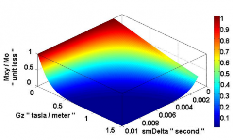
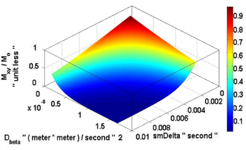
Figure 35. Stretched exponential model surface plot:
$\mathrm{M}_{\mathrm{xy}} / \mathrm{M}_{\mathrm{o}} \text { Versus } \mathrm{D}_{\beta} \text { where } \mathrm{D}_{\beta}=1.7 \times 10^{-3} \text {to } 16.7 \times 10^{-3} \mathrm{~mm}^{2} / \mathrm{s}, \text { and } \delta \text { where } \delta=1 \times 10^{-3} \text {to } 10 \times 10^{-3} \mathrm{~s}$.
$\left(\mu=2 \mu \mathrm{m}, \beta=0.6, \mathrm{G}_{\mathrm{z}}=1.5 \mathrm{~T} / \mathrm{m}, \Delta=40 \times 10^{-3} \mathrm{~s}, \gamma=42.58 \mathrm{MHz} / \mathrm{T}\right)$
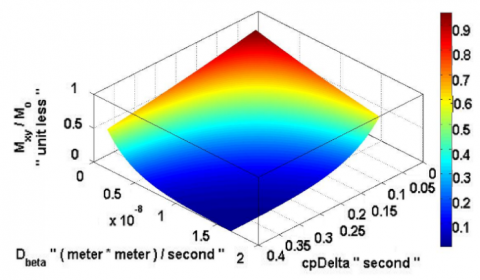
Figure 36. Stretched exponential model surface plot:
$\mathrm{M}_{\mathrm{xy}} / \mathrm{M}_{\mathrm{o}} \text { Versus } \mathrm{D}_{\beta} \text { where } \mathrm{D}_{\beta}=1.7 \times 10^{-3} \text {to } 16.7 \times 10^{-3} \mathrm{~mm}^{2} / \mathrm{s}, \text { and } \Delta \text { where } \Delta=40 \times 10^{-3} \text {to } 400 \times 10^{-3} \mathrm{~s}$.
$\left(\mu=2 \mu \mathrm{m}, \beta=0.6, \mathrm{G}_{\mathrm{z}}=1.5 \mathrm{~T} / \mathrm{m}, \delta=1 \times 10^{-3} \mathrm{~s}, \gamma=42.58 \mathrm{MHz} / \mathrm{T}\right)$
Another example of the behavior expected, the decay of the normalized magnetization $\left(M_{x y} / M_{0}\right),$ is plotted in Figure 14 versus $\overline{\mathrm{b}}$ factor where $\overline{\mathrm{b}}$ factor $=0$ to $250 \mathrm{~s} / \mathrm{mm}^{2}$ and $\overline{\mathrm{b}}$ factor $=\frac{1}{\beta \mu_{\beta}^{2}}\left(\gamma \mathrm{G}_{\mathrm{z}} \delta \beta \mu_{\beta}\right)^{2 \beta}\left(\Delta-\frac{2 \beta-1}{2 \beta+1} \delta\right)$ for $\quad$ different values of $\beta$ in the range from $\beta=0.6$ (bottom curve) to $\beta=0.9$ in steps of $0.1\left(\mathrm{D}=1^{*} 10^{-3} \mathrm{~mm}^{2} / \mathrm{s}, \mu=5 \mu \mathrm{m}, G_{\mathrm{z}}=\right.$ 0 to $\left.1.5 \mathrm{~T} / \mathrm{m}, \delta=1 \times 10^{-3} \mathrm{~s}, \Delta=40 \times 10^{-3} \mathrm{~s}, \gamma=42.58 \mathrm{MHz} / \mathrm{T}\right)$.
In Figure $15,$ Eq. ( 2 ) normalized magnetization $\mathrm{M}_{\mathrm{xy}} / \mathrm{M}_{\mathrm{o}}$ versus $\mathrm{G}_{\mathrm{z}}$ was plotted where $\mathrm{G}_{\mathrm{z}}=0$ to $1.5 \mathrm{~T} / \mathrm{m}$ and $\mu$ where $\mu$ $=2$ to $10 \mu \mathrm{m} .\left(\mathrm{D}=1 \times 10^{-3} \mathrm{~mm}^{2} / \mathrm{s}, \beta=0.6, \delta=1 \times 10^{-3} \mathrm{~s}, \Delta=\right.$$\left.40 \times 10^{-3} \mathrm{~s}, \gamma=42.58 \mathrm{MHz} / \mathrm{T}\right)$. In Figure $16,$ Eq. ( 2 ) normalized magnetization $\mathrm{M}_{\mathrm{xy}} / \mathrm{M}_{\mathrm{o}}$ versus $\beta$ was plotted where, $\beta=0.5$ to 1 and $\mu$ where $\mu=2$ to $10 \mu \mathrm{m} \cdot\left(\mathrm{D}=1 \times 10^{-3} \mathrm{~mm}^{2} / \mathrm{s}, \mathrm{G}_{\mathrm{z}}=1.5 \mathrm{~T} / \mathrm{m}, \delta=1 \times 10^{-3} \mathrm{~s}, \Delta=\right.$$\begin{array}{ccccc}40 \times & 10^{-3} \mathrm{~s}, & \gamma= & 42.58 & \mathrm{MHz} / \mathrm{T}) & \text { In Figure } & 17, \text { Eq. }\end{array}$ normalized magnetization $\mathrm{M}_{\mathrm{xy}} / \mathrm{M}_{\mathrm{o}}$ Versus $\mathrm{D}$ was plotted where $\mathrm{D}=1 \times 10^{-3}$ to $10 \times 10^{-3} \mathrm{~mm}^{2} / \mathrm{s}$ and $\mu$ where $\mu=2$ to $10 \mu \mathrm{m} .\left(\beta=0.6, \mathrm{G}_{\mathrm{z}}=1.5 \mathrm{~T} / \mathrm{m}, \delta=1 \times 10^{-3} \mathrm{~s}, \Delta=40 \times 10^{-3} \mathrm{~s}\right.$ $\gamma=42.58 \mathrm{MHz} / \mathrm{T})$. In Figure $18,$ Eq. ( 2 ) normalized magnetization $\mathrm{M}_{\mathrm{xy}} / \mathrm{M}_{\mathrm{o}}$ versus $\beta$ was plotted where $\beta=0.5$ to 1 and $D$ where $D=1$ $\times 10^{-3}$ to $10 \times 10^{-3} \mathrm{~mm}^{2} / \mathrm{s} .\left(\mu=2 \times 10^{-6} \mathrm{~m}, \mathrm{G}_{\mathrm{z}}=1.5 \mathrm{~T} / \mathrm{m}\right.$ $\left.\delta=1 \times 10^{-3} \mathrm{~s}, \Delta=40 \times 10^{-3} \mathrm{~s}, \gamma=42.58 \mathrm{MHz} / \mathrm{T}\right) .$ In Figure 19 Eq. (2) normalized magnetization $\mathrm{M}_{\mathrm{xy}} / \mathrm{M}_{\mathrm{o}}$ versus $\beta$ was plotted where $\beta=0.5$ to 1 and $\Delta$ where $\Delta=40 \times 10^{-3}$ to 400 $\times 10^{-3} \mathrm{~s} .\left(\mu=2 \times 10^{-6} \mathrm{~m}, \mathrm{G}_{\mathrm{z}}=1.5 \mathrm{~T} / \mathrm{m}, \delta=1 \times 10^{-3} \mathrm{~s}, \mathrm{D}=\right.$ $\left.1 \times 10^{-3} \mathrm{~mm}^{2} / \mathrm{s}, \gamma=42.58 \mathrm{MHz} / \mathrm{T}\right)$. In Figure $20,$ Eq. (2) normalized magnetization $\mathrm{M}_{\mathrm{xy}} / \mathrm{M}_{\mathrm{o}}$ versus $\beta$ was plotted where $\beta=0.5$ to 1 and $\delta$ where $\delta=1$ $\times 10^{-3}$ to $10 \times 10^{-3} \mathrm{~s} .\left(\mu=2 \times 10^{-6} \mathrm{~m}, \mathrm{G}_{\mathrm{z}}=1.5 \mathrm{~T} / \mathrm{m}, \Delta=\right.$ $\left.40 \times 10^{-3} \mathrm{~s}, \mathrm{D}=1 \times 10^{-3} \mathrm{~mm}^{2} / \mathrm{s}, \gamma=42.58 \mathrm{MHz} / \mathrm{T}\right)$. In Figure $21,$ Eq. ( 2 ) normalized magnetization $\mathrm{M}_{\mathrm{xy}} / \mathrm{M}_{\mathrm{o}}$ versus $\Delta$ was plotted where $\Delta=40 \times 10^{-3}$ to $400 \times 10^{-3} \mathrm{~s}$ and $\delta$ where $\delta=1 \times 10^{-3}$ to $10 \times 10^{-3} \mathrm{~s} .\left(\mu=2 \times 10^{-6} \mathrm{~m}, \mathrm{G}_{\mathrm{z}}=1.5\right.$ $\left.\mathrm{T} / \mathrm{m}, \beta=0.6, \mathrm{D}=1 \times 10^{-3} \mathrm{~mm}^{2} / \mathrm{s}, \gamma=42.58 \mathrm{MHz} / \mathrm{T}\right)$. In Figure 22 Eq. ( 2 ) normalized magnetization $\mathrm{M}_{\mathrm{xy}} / \mathrm{M}_{\mathrm{o}}$ versus $\mathrm{G}_{\mathrm{z}}$ was plotted where $\mathrm{G}_{\mathrm{z}}=0$ to $1.5 \mathrm{~T} / \mathrm{m}$ and $\beta$ where $\beta$ $=0.5$ to $1 .\left(\mu=2 \times 10^{-6} \mathrm{~m}, \Delta=40 \times 10^{-3} \mathrm{~s}, \delta=1 \times 10^{-3} \mathrm{~s}, \mathrm{D}\right.$ $\left.=1 \times 10^{-3} \mathrm{~mm}^{2} / \mathrm{s}, \gamma=42.58 \mathrm{MHz} / \mathrm{T}\right)$. In Figure 23 Eq. (2) normalized magnetization $\mathrm{M}_{\mathrm{xy}} / \mathrm{M}_{\mathrm{o}}$ versus $\mathrm{G}_{\mathrm{z}}$ was plotted where $\mathrm{G}_{\mathrm{z}}=0$ to $1.5 \mathrm{~T} / \mathrm{m}$ and $\Delta$ where $\Delta$ $=40 \times 10^{-3}$ to $40 \times 10^{-3} \mathrm{~s} .\left(\mu=2 \times 10^{-6} \mathrm{~m}, \beta=0.6, \delta=\right.$ $\left.1 \times 10^{-3} \mathrm{~s}, \mathrm{D}=1 \times 10^{-3} \mathrm{~mm}^{2} / \mathrm{s}, \gamma=42.58 \mathrm{MHz} / \mathrm{T}\right)$. In Figure 24 Eq. (2) normalized magnetization $\mathrm{M}_{\mathrm{xy}} / \mathrm{M}_{\mathrm{o}}$ versus $\mathrm{G}_{\mathrm{z}}$ was plotted where $\mathrm{G}_{\mathrm{z}}=0$ to $1.5 \mathrm{~T} / \mathrm{m}$ and $\delta$ where $\delta$ $=1 \times 10^{-3}$ to $10 \times 10^{-3} \mathrm{~s} \cdot\left(\mu=2 \times 10^{-6} \mathrm{~m}, \beta=0.6, \Delta=\right.$ $\left.40 \times 10^{-3} \mathrm{~s}, \mathrm{D}=1 \times 10^{-3} \mathrm{~mm}^{2} / \mathrm{s}, \gamma=42.58 \mathrm{MHz} / \mathrm{T}\right)$. In Figure 25 Eq. (2) normalized magnetization $\mathrm{M}_{\mathrm{xy}} / \mathrm{M}_{\mathrm{o}}$ versus $\mathrm{G}_{\mathrm{z}}$ was plotted where $\mathrm{G}_{\mathrm{z}}=0$ to $1.5 \mathrm{~T} / \mathrm{m}$ and $\mathrm{D}$ where $\mathrm{D}$ $=1 \times 10^{-3}$ to $10 \times 10^{-3} \mathrm{~mm}^{2} / \mathrm{s} .\left(\mu=2 \times 10^{-6} \mathrm{~m}, \beta=0.6, \Delta=\right.$ $\left.40 \times 10^{-3} \mathrm{~s}, \delta=1 \times 10^{-3} \mathrm{~s}, \gamma=42.58 \mathrm{MHz} / \mathrm{T}\right)$. In Figure 26 Eq. (2) normalized magnetization $\mathrm{M}_{\mathrm{xy}} / \mathrm{M}_{\mathrm{o}}$ versus $\delta$ was plotted where $\delta=1 \times 10^{-3}$ to $10 \times 10^{-3} \mathrm{~s}$ and $\mathrm{D}$ where $\mathrm{D}=1 \times 10^{-3}$ to $10 \times 10^{-3} \mathrm{~mm}^{2} / \mathrm{s} .\left(\mu=2 \times 10^{-6} \mathrm{~m}, \beta=\right.$ $\left.0.6, \Delta=40 \times 10^{-3} \mathrm{~s}, \mathrm{G}_{\mathrm{z}}=1.5 \mathrm{~T} / \mathrm{m}, \gamma=42.58 \mathrm{MHz} / \mathrm{T}\right)$. In Figure 27 Eq. (2) normalized magnetization $\mathrm{M}_{\mathrm{xy}} / \mathrm{M}_{\mathrm{o}}$ versus $\delta$ was plotted where $\Delta=40 \times 10^{-3}$ to $400 \times 10^{-3} \mathrm{~s}$ and $\mathrm{D}$ where $\mathrm{D}=1 \times 10^{-3}$ to $10 \times 10^{-3} \mathrm{~mm}^{2} / \mathrm{s} .\left(\mu=2 \times 10^{-6} \mathrm{~m}, \beta\right.$ $\left.=0.6, \delta=1 \times 10^{-3} \mathrm{~s}, \mathrm{G}_{\mathrm{z}}=1.5 \mathrm{~T} / \mathrm{m}, \gamma=42.58 \mathrm{MHz} / \mathrm{T}\right)$. In Figure 28 Eq. (2) normalized magnetization $\mathrm{M}_{\mathrm{xy}} / \mathrm{M}_{\mathrm{o}}$ versus $\delta$ was plotted where $\delta=1 \times 10^{-3}$ to $10 \times 10^{-3} \mathrm{~s}$ and $\mu$ where $\mu=2$ to $10 \mu \mathrm{m} .\left(\mathrm{D}=1 \times 10^{-3} \mathrm{~mm}^{2} / \mathrm{s}, \beta=0.6, \Delta=\right.$ $\left.40 \times 10^{-3} \mathrm{~s}, \mathrm{G}_{7}=1.5 \mathrm{~T} / \mathrm{m}, \gamma=42.58 \mathrm{MHz} / \mathrm{T}\right)$. In Figure 29 Eq. (2) normalized magnetization $\mathrm{M}_{\mathrm{xy}} / \mathrm{M}_{\mathrm{o}}$ versus $\Delta$ was plotted where $\Delta=40 \times 10^{-3}$ to $400 \times 10^{-3} \mathrm{~s}$ and $\mu$ where $\mu=2$ to $10 \mu \mathrm{m} .\left(\mathrm{D}=1 \times 10^{-3} \mathrm{~mm}^{2} / \mathrm{s}, \beta=0.6, \delta=\right.$ $\left.1 \times 10^{-3} \mathrm{~s}, \mathrm{G}_{\mathrm{z}}=1.5 \mathrm{~T} / \mathrm{m}, \gamma=42.58 \mathrm{MHz} / \mathrm{T}\right)$. In Figure 30 Eq. (2) normalized magnetization $\mathrm{M}_{\mathrm{xy}} / \mathrm{M}_{\mathrm{o}}$ versus $\mathrm{G}_{\mathrm{z}}$ was plotted where $\mathrm{G}_{\mathrm{z}}=0$ to $1.5 \mathrm{~T} / \mathrm{m}$ and $\mu_{\beta}$ where $\mu_{\beta}=0.333 \times 10^{-5}$ to $1.67 \times 10^{-5} \mathrm{~m} \cdot\left(\mathrm{D}=1 \times 10^{-3} \mathrm{~mm}^{2} / \mathrm{s}, \beta=\right.$ $\left.0.6, \delta=1 \times 10^{-3} \mathrm{~s}, \Delta=40 \times 10^{-3} \mathrm{~s}, \gamma=42.58 \mathrm{MHz} / \mathrm{T}\right)$. In Figure 31 Eq. ( 2 ) normalized magnetization $\mathrm{M}_{\mathrm{xy}} / \mathrm{M}_{\mathrm{o}}$ versus $\beta$ was plotted where $\beta=0.5$ to 1 and $\mu_{\beta}$ where $\mu_{\beta}$ $=0.333 \times 10^{-5}$ to $1.67 \times 10^{-5} \mathrm{~m} .\left(\mathrm{D}=1 \times 10^{-3} \mathrm{~mm}^{2} / \mathrm{s}, \mathrm{G}_{\mathrm{z}}=\right.$ $\left.1.5 \mathrm{~T} / \mathrm{m}, \delta=1 \times 10^{-3} \mathrm{~s}, \Delta=40 \times 10^{-3} \mathrm{~s}, \gamma=42.58 \mathrm{MHz} / \mathrm{T}\right)$. In Figure 32 Eq. (2) normalized magnetization $\mathrm{M}_{\mathrm{xy}} / \mathrm{M}_{\mathrm{o}}$ versus $D_{\beta}$ was plotted where $D_{\beta}=1.7 \times 10^{-3}$ to $16.7 \times$ $10^{-3} \mathrm{~mm}^{2} / \mathrm{s},$ and $\mu_{\beta}$ where $\mu_{\beta}=3.33 \times 10^{-5}$ to $1.67 \times$ $10^{-5} \mathrm{~m} \cdot\left(\beta=0.6, \mathrm{G}_{\mathrm{z}}=1.5 \mathrm{~T} / \mathrm{m}, \delta=1 \times 10^{-3} \mathrm{~s}, \Delta=40 \times\right.$ $\left.10^{-3} \mathrm{~s}, \gamma=42.58 \mathrm{MHz} / \mathrm{T}\right)$. In Figure 33 Eq. (2) normalized magnetization $\mathrm{M}_{\mathrm{xy}} / \mathrm{M}_{\mathrm{o}}$ versus $D_{\beta}$ was plotted where $D_{\beta}=1.7 \times 10^{-3}$ to $16.7 x$ $10^{-3} \mathrm{~mm}^{2} / \mathrm{s},$ and $\beta$ where $\beta=0.5$ to $1 .\left(\mu=2 \mu \mathrm{m}, \mathrm{G}_{\mathrm{z}}=1.5\right.$ $\left.\mathrm{T} / \mathrm{m}, \delta=1 \times 10^{-3} \mathrm{~s}, \Delta=40 \times 10^{-3} \mathrm{~s}, \gamma=42.58 \mathrm{MHz} / \mathrm{T}\right)$. In Figure 34 Eq. (2) normalized magnetization $\mathrm{M}_{\mathrm{xy}} / \mathrm{M}_{\mathrm{o}}$ versus $D_{\beta}$ was plotted where $D_{\beta}=1.7 \times 10^{-3}$ to $16.7 \times$ $10^{-3} \mathrm{~mm}^{2} / \mathrm{s},$ and $\mathrm{G}_{\mathrm{z}}$ where $\mathrm{G}_{\mathrm{z}}=0$ to $1.5 \mathrm{~T} / \mathrm{m} .(\mu=2 \mu \mathrm{m}, \beta=$ $\left.0.6, \delta=1 \times 10^{-3} \mathrm{~s}, \Delta=40 \times 10^{-3} \mathrm{~s}, \gamma=42.58 \mathrm{MHz} / \mathrm{T}\right)$. In Figure 35 Eq. (2) normalized magnetization $\mathrm{M}_{\mathrm{xy}} / \mathrm{M}_{\mathrm{o}}$ versus $\mathrm{D}_{\beta}$ was plotted where $\mathrm{D}_{\beta}=1.7 \times 10^{-3}$ to $16.7 \times$ $10^{-3} \mathrm{~mm}^{2} / \mathrm{s},$ and $\delta$ where $\delta=1 \times 10^{-3}$ to $10 \times 10^{-3} \mathrm{~s} .(\mu=$ $\left.2 \mu \mathrm{m}, \beta=0.6, \mathrm{G}_{\mathrm{z}}=1.5 \mathrm{~T} / \mathrm{m}, \Delta=40 \times 10^{-3} \mathrm{~s}, \gamma=42.58 \mathrm{MHz} / \mathrm{T}\right)$. In Figure 36 Eq. (2) normalized magnetization $\mathrm{M}_{\mathrm{xy}} / \mathrm{M}_{\mathrm{o}}$ versus $D_{\beta}$ was plotted where $D_{\beta}=1.7 \times 10^{-3}$ to $16.7 \times$ $10^{-3} \mathrm{~mm}^{2} / \mathrm{s},$ and $\Delta$ where $\Delta=40 \times 10^{-3}$ to $400 \times 10^{-3} \mathrm{~s} .(\mu=$ $\left.2 \mu \mathrm{m}, \beta=0.6, \mathrm{G}_{\mathrm{z}}=1.5 \mathrm{~T} / \mathrm{m}, \delta=1 \times 10^{-3} \mathrm{~s}, \gamma=42.58 \mathrm{MHz} / \mathrm{T}\right)$. In Figure 37 Eq. (2) normalized magnetization $\mathrm{M}_{\mathrm{xy}} / \mathrm{M}_{\mathrm{o}}$ versus $\delta$ was plotted where $\delta=1 \times 10^{-3}$ to $10 \times 10^{-3} \mathrm{~s}$ and $\mu_{\beta}$ where $\mu_{\beta}=0.333 \times 10^{-5}$ to $1.67 \times 10^{-5} \mathrm{~m} . \quad(\mathrm{D}=1 \times$ $10^{-3} \mathrm{~mm}^{2} / \mathrm{s}, \mathrm{G}_{\mathrm{z}}=1.5 \mathrm{~T} / \mathrm{m}, \beta=0.6, \Delta=40 \times 10^{-3} \mathrm{~s}, \gamma=42.58$ $\mathrm{MHz} / \mathrm{T})$. Finally, in Figure 38 Eq. (2) the normalized magnetization $\mathrm{M}_{\mathrm{xy}} / \mathrm{M}_{\mathrm{o}} \text { versus } \Delta \text { was plotted where } \Delta=40 \times 10^{-3}$ to 400 $\times 10^{-3} \mathrm{~s} \text { and } \mu_{\beta} \text { where } \mu_{\beta}=0.333 \times 10^{-5} \text {to } 1.67 \times 10^{-5} \mathrm{~m}$ $\left(\mathrm{D}=1 \times 10^{-3} \mathrm{~mm}^{2} / \mathrm{s}, \mathrm{G}_{\mathrm{z}}=1.5 \mathrm{~T} / \mathrm{m}, \beta=0.6, \delta=1 \times 10^{-3} \mathrm{~s}, \gamma=42.58 \mathrm{MHz} / \mathrm{T}\right)$.
Figure 37. Stretched exponential model surface plot:
$\mathrm{M}_{\mathrm{xy}} / \mathrm{M}_{\mathrm{o}} \text { Versus } \delta \text { where } \delta=1 \times 10^{-3} \text {to } 10 \times 10^{-3} \mathrm{~s} \text { and } \mu_{\beta} \text { where } \mu_{\beta}=0.333 \times 10^{-5} \text {to } 1.67 \times 10^{-5} \mathrm{~m}$.
$\left(\mathrm{D}=1 \times 10^{-3} \mathrm{~mm}^{2} / \mathrm{s}, \mathrm{G}_{\mathrm{z}}=1.5 \mathrm{~T} / \mathrm{m}, \beta=0.6, \Delta=40 \times 10^{-3} \mathrm{~s}, \gamma=42.58 \mathrm{MHz} / \mathrm{T}\right)$
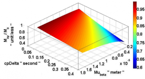
Figure 38. Stretched exponential model surface plot:
$\mathrm{M}_{\mathrm{xy}} / \mathrm{M}_{\mathrm{o}} \text { Versus } \Delta \text { where } \Delta=40 \times 10^{-3} \mathrm{to} 400 \times 10^{-3} \mathrm{~s} \text { and } \mu_{\beta} \text { where } \mu_{\beta}=0.333 \times 10^{-5} \text {to } 1.67 \times 10^{-5} \mathrm{~m}$.
$\left(\mathrm{D}=1 \times 10^{-3} \mathrm{~mm}^{2} / \mathrm{s}, \mathrm{G}_{\mathrm{z}}=1.5 \mathrm{~T} / \mathrm{m}, \beta=0.6, \delta=1 \times 10^{-3} \mathrm{~s}, \gamma=42.58 \mathrm{MHz} / \mathrm{T}\right)$
In this paper we discuss the stretch function resulting from solving the generalize fractional-order Bloch equations using fractional calculus in details. The theoretical curves were plotted versus the gradient parameter, $\text { bfactor, b'factor, } \overline{\mathrm{b}} \text { factor, Sfactor, } \mathrm{b}^{*} \text { factor and } \mathrm{G}_{\mathrm{z}}$ for selected values of ∆, δ, $\mathrm{G}_{\mathrm{z}}$, β and µ. Stretched exponential function surface plot were also plotted, different shapes of decays were observed versus different values of $\text { bfactor, b'factor, } \overline{\mathrm{b}} \text { factor, Sfactor, } \mathrm{b}^{*} \text { factor and } \mathrm{G}_{\mathrm{z}}$ for selected values of ∆, δ, $\mathrm{G}_{\mathrm{z}}$, β and µ.
We observe that the stretch function resulting from solving the generalize fractional-order Bloch equations behaves like pure exponential function with rats $\mathrm{D}_{\beta} \text { when we use } \bar{b} \text { factor }$, and behaves like stretch exponential function inside power law when we use $\text { S factor and X factor }$. Further developments of this study may be useful in optimizing anomalous diffusion in tissues with neurodegenerative, and ischemic diseases.
This work is supported by The Hashemite University and The University of Illinois at Chicago.
[1] Magin, R.L., Abdullah, O., Baleanu, D., Zhou, X.J. (2008). Anomalous diffusion expressed through fractional order differential operators in the Bloch-Torrey equation. Journal of Magnetic Resonance, 190(2): 255-270. https://doi.org/10.1016/j.jmr.2007.11.007
[2] Kopf, M., Metzler, R., Haferkamp, O., Nonnenmacher, T.F. (1998). NMR studies of anomalous diffusion in biological tissues: Experimental observation of Levy stable processes. In: G.A. Losa, D. Merlini, T.F. Nonnenmacher, E.R. Weibel (Eds.), Fractals in Biology and Medicine, vol. II, Birkhauser, Basel, 345-364. https://doi.org/10.1007/978-3-0348-8936-0_28
[3] Kilbas, A.A., Srivastava, H.M., Trujillo, J.J. (2006). Theory and Applications of Fractional Differential Equations. Elsevier, Amsterdam.
[4] Metzler, R., Nonnenmacher, T.F. (2002). Space- and time-fractional diffusion and wave equations, fractional Fokker–Planck equations, and physical motivation. Chemical Physics, 284(1-2): 67-90. https://doi.org/10.1016/S0301-0104(02)00537-2
[5] Callaghan, P.T. (2011). Translational Dynamics and Magnetic Resonance: Principles of Pulsed Gradient Spin Echo NMR. Oxford: Oxford University Press. https://doi.org/10.1093/acprof:oso/9780199556984.001.0001
[6] Zhou, X.J., Gao, Q., Abdullah, O., Magin, R.L. (2010). Studies of anomalous diffusion in the human brain using fractional order calculus. Magnetic Resonance in Medicine, 63(3): 562-569. https://doi.org/10.1002/mrm.22285
[7] Kuchel, P.W., Pages, G., Nagashima, K., Sendhil, V., Vijayaragavan, V., Nagarajan, V., Chuang, K.H. (2012). Stejskal–Tanner equation derived in full. Conc Magn Reson. 40A(5): 205-214. https://doi.org/10.1002/cmr.a.21241
[8] Magin, R.L., Xu, F., Baleanu, D. (2008). Solving the fractional order Bloch equation. Conc Magn Reson., 34A(1): 16-23. https://doi.org/10.1002/cmr.a.20129
[9] Berberan-Santos, M.N. (2008). A luminescence decay function encompassing the stretched exponential and the compressed hyperbola. Chemical Physics Letters, 460(1-3): 146-150. https://doi.org/10.1016/j.cplett.2008.06.023
[10] Berberan-Santos, M.N., Valeur, B. (2007). Luminescence decays with underlying distributions: general properties and analysis with mathematical functions. Journal of Luminescence, 126(2): 263-272. https://doi.org/10.1016/j.jlumin.2006.07.004
[11] Marchenko, V.A. (1986). Sturm–Liouville Operators and Applications. Birkhäuser.
[12] Nomura, Y., Sakuma, H., Takeda, K., Tagami, T., Okuda, Y., Nakagawa, T. (1994). Diffusional anisotropy of the human brain assessed with diffusion-weighted MR: relation with normal brain development and aging. AJNR, 15(2): 231-238.
[13] Berberan-Santos, M.N., Bodunov, E.N., Valeur, B. (2005). Mathematical functions for the analysis of luminescence decays with underlying distributions: 2. Becquerel (compressed hyperbola) and related decay functions. Chemical Physics, 317(1): 57-62. https://doi.org/10.1016/j.chemphys.2005.05.026
[14] Machta, B.B., Chachra, R., Transtrum, M.K., Sethna, J.P. Parameter space compression underlies emergent theories and predictive models. Science, 342(6158): 604-607. https://doi.org/10.1126/science.1238723
[15] Rozov, N.K.H. (2001). Singular solution. Encyclopedia of Mathematics, Springer Science, Business Media B.V. / Kluwer Academic Publishers.
[16] Phillips, E.G. (1957). Functions of a Complex Variable with Applications, 8th ed. Edinburgh: Oliver and Boyd.
[17] Basser, P., Pierpaoli, C. (1996). Microstructural and physiological features of tissues elucidated by quantitative-diffusion-tensor MRI. Journal of Magnetic Resonance, Series B, 111(3): 209-219. https://doi.org/10.1006/jmrb.1996.0086
[18] ennett, K.M., Schmainda, K.M., Bennett, R.T., Rowe, D.B., Lu, H., Hyde, J.S. (2003). Characterization of continuously distributed cortical water diffusion rates with a stretched-exponential model. Magn. Reson. Med., 50(4): 727-734. https://doi.org/10.1002/mrm.10581
[19] Bennett, K.M., Hyde, J.S., Schmainda, K.M. (2006). Water diffusion heterogeneity index in the human brain is insensitive to the orientation of applied magnetic field gradients. Magn. Reson. Med., 56(2): 235-239. https://doi.org/10.1002/mrm.20960
[20] Clark, C.A., Le Bihan, D. (2020). Water diffusion compartmentation and anisotropy at high B values in the human brain. Magn. Reson. Med., 44(6): 852-859. https://doi.org/10.1002/1522-2594(200012)44:6<852::aid-mrm5>3.0.co;2-a