Hamed Reza Zarif Sanayei* | Fatemeh Nasiri
© 2020 IIETA. This article is published by IIETA and is licensed under the CC BY 4.0 license (http://creativecommons.org/licenses/by/4.0/).
OPEN ACCESS
In hydraulic engineering, the steady non-uniform flow in a channel with the gradual changes at the water surface level is introduced as the Gradually Varied Flow (GVF). For the design of open channels, it is necessary to calculate the GVF profile along the channel flow. The GVF profile is described by a nonlinear Ordinary Differential Equation (ODE). Because this equation is strongly nonlinear, providing new analytical and/or semi-analytical solutions for this equation without any simplifications and/or linearizations would be necessary and helpful. In this research, the Perturbation Method (PM) is proposed to present a semi-analytical solution for solving the GVF equation in the prismatic triangular channel. A total of two cases are studied in this paper. In case 1, the Manning equation and in case 2, the Chezy equation are applied as the resistance equations. The GVF profiles in the two cases are compared with the Finite Difference Method (FDM) profiles. Also, the effect of the summation truncation in the PM is studied for these cases. The results show that by increasing the terms approximation in the PM, the GVF profile converges to the FDM profile. A reference solution for efficiency assessment of numerical techniques can be provided by presented semi-analytical solutions in this paper. Furthermore, the proposed method in this paper can be used as a new idea in providing semi-analytical solutions to other open channel works.
gradually varied flow, nonlinear ordinary differential equation, perturbation method, semi-analytical solution, triangular channel, water surface profile
In a prismatic channel, the steady non-uniform flow with gradual changes at the water surface level is defined as Gradually varied flow (GVF) [1]. For the design of open channels, it is necessary to calculate the water depth along the flow direction and it is performed by investigation of GVF in the channel.
Over the past few decades, the calculation of GVF profiles has been an important issue for hydraulic engineering. To obtain this profile, the nonlinear ordinary differential equation of the GVF should be solved. Analytical and numerical methods can be used for the solution of this equation. However, due to the extreme nonlinear state of this equation, providing an analytical solution for it is difficult. In the last three decades, many numerical techniques have been proposed to obtain a GVF profile in the open channels.
Numerical techniques consist of Finite Difference Method (FDM), Newton-Raphson method, Differential Quadrature Method (DQM), Runge– Kutta method, Genetic Programming and other methods [2-16].
However, numerical methods that have been proposed for solving this problem are discontinuous solutions. Analytical and semi-analytical solutions continue and give a proper understanding for problems, compared to numerical solutions. Analytical solutions can be used as reference solutions for verifying numerical solutions and numerical programming [17, 18]. Patil et al. [19] introduced an improved direct method for the Chow method in prismatic channels to solve the GVF equation. The hydraulic parameters in their integration were considered to be variable, unlike the Chow method that the hydraulic parameters were constant at all depths. Vatankhah [20] presented an analytical solution for calculation of the GVF profile length in triangular channels using the Manning formula as the resistance equation. He obtained the GVF profiles for subcritical and supercritical flows in the Mild and steep slopes. Jan and Chen [21] applied the Gaussian hyper-geometric function (GHF) in the direct integration method for the analytical solution of the GVF equation in sustain and non-sustain wide channels. They obtained the GHF-based solutions for GVF profiles in various slopes. Vatankhah [22] developed an analytical solution by the direct integration method to obtain the GVF profile in the circular prismatic channels. He applied the variable Manning coefficient in the governing equation. Tajari et al. [23] presented the semi-analytical solution and numerical simulation for the spatially varied flow (SVF) equation along duckbill weir. In that paper, the semi-analytical solution and Flow-3D simulation were in good agreement with experimental results.
Homayoon and Abedini [24] presented an analytical solution to the GVF equation for ordinary rectangular and triangular channels with the Manning equation as the resistance equation. The proposed analytical solution was compared with HEC-RAS software and numerical integration schemes.
Other similar researches investigated the analytical and semi-analytical solutions for GVF profiles in various channels [25-33].
Analytical solutions presented in the literature for the governing equation contain many simplifications. Therefore, providing new analytical and/or semi-analytical solutions for the GVF profile equation without such simplifications and/or linearizations would be necessary and helpful. In addition, most presented methods to date only provide the profile length between two specified water depths along the channel. In other words, they do not provide any closed form continuous equation for the profile or water surface along the channel.
In this research, the Perturbation Method (PM) is proposed to present a semi-analytical solution for solving the GVF equation in the prismatic triangular channels. A total of two cases are investigated in this study. In case 1, the Manning equation and in case 2, the Chezy equation are utilized as the resistance equations. The GVF profiles in two cases are compared with the Finite Difference Method (FDM) profiles. Also, the effect of the terms approximation and the summations truncation in the PM is studied for these cases. These semi-analytical solutions may be used as a benchmark for verification and efficiency assessment of other numerical approaches.
The Governing equation and boundary condition for the GVF in a prismatic channel may be expressed as [34, 35].
$\frac{d y}{d x}=\frac{S_{0}-S_{f}}{1-F r^{2}}, \quad y(0)=y_{1}$ (1)
where, x is the distance along the channel (positive in the direction of channel flow); y is the water depth; S0 is the longitudinal slope of the channel; Sf is the energy line slope and Fr is the Froude number. The Fr2 for the triangular channel is:
$F r^{2}=\frac{Q^{2} T}{g A^{3}}=\frac{Q^{2}(2 Z y)}{g\left(Z y^{2}\right)^{3}}=\frac{2 Q^{2}}{g Z^{2} y^{5}}=G(y)$ (2)
where, Q is the discharge; A is the cross section area of the channel flow; T is the width of the water surface; g is the acceleration of gravitation and Z is the side slope of the triangular channel. For simplicity, Fr2 is replaced with G(y) in the next equations.
At first, Eq. (1) is rearranged as follows:
$\frac{d x}{d y}=\frac{1-F r^{2}}{S_{0}-S_{f}}, \quad x\left(y_{1}\right)=0$ (3)
In Eq. (3), Sf is substituted by the Manning equation for the triangular channel.
According to the perturbation method, a solution for the Eq. (3) is presented as [36]:
$x(y, \varepsilon)=\sum_{k=0}^{m} \varepsilon^{k} x_{k}(y)+o\left(\varepsilon^{m+1}\right)$. (4)
where, ε is a small parameter that can be artificially introduced in the governing equation (Eq. (3)).
Some terms of the perturbation series (Eq. (4)) for ε=1 may be written as:
$x(y)=x_{0}(y)+x_{1}(y)+x_{2}(y)+\ldots$ (5)
In this research, the ε parameter is inserted into Eq. (3) as follows:
$\frac{d x}{d y}=\frac{1-F r^{2}}{S_{0}-\varepsilon S_{f}}$ (6a)
$x\left(y_{1}\right)=0$ (6b)
Now, substituting Eq. (4) into Eq. (6a) (rearranged ODE with the ε parameter) and applying some simplifications yields:
$\left(S_{0}-\varepsilon \frac{n^{2} Q^{2}}{f(y)}\right)\left(x_{0}^{\prime}+\varepsilon x_{1}^{\prime}+\varepsilon^{2} x_{2}^{\prime}+\varepsilon^{3} x_{3}^{\prime}+\ldots\right)=1-G(y)$ (7)
where, n is Manning roughness coefficient and f(y) is:
$f(y)=\left(\frac{Z y}{2 \sqrt{1+Z^{2}}}\right)^{4 / 3} Z^{2} y^{4}=R^{4 / 3} Z^{2} y^{4}$ (8)
Also, substituting Eq. (4) into rearranged boundary condition (Eq. (6b)) gives:
$\varepsilon^{0} x_{0}\left(y_{1}\right)+\varepsilon^{1} x_{1}\left(y_{1}\right)+\varepsilon^{2} x_{2}\left(y_{1}\right)+\varepsilon^{3} x_{3}\left(y_{1}\right)+\ldots=0$ (9)
Equating the left and right side terms of Eqns. (7) and (9) for identical powers of ε0, ε1, ε2, ε3, … and applying some simplifications yields:
$\varepsilon^{0}: S_{0} f(y) x_{0}^{\prime}=f(y)-G(y) f(y), x_{0}\left(y_{1}\right)=0$ (10a)
$\varepsilon^{1}: S_{0} f(y) x_{1}^{\prime}=n^{2} Q^{2} x_{0}^{\prime}, \quad x_{1}\left(y_{1}\right)=0$ (10b)
$\varepsilon^{2}: S_{0} f(y) x_{2}^{\prime}=n^{2} Q^{2} x_{1}^{\prime}, \quad x_{2}\left(y_{1}\right)=0$ (10c)
$\varepsilon^{3}: S_{0} f(y) x_{3}^{\prime}=n^{2} Q^{2} x_{2}^{\prime}, \quad x_{3}\left(y_{1}\right)=0$ (10d)
$\varepsilon^{4}: S_{0} f(y) x_{4}^{\prime}=n^{2} Q^{2} x_{3}^{\prime}, \quad x_{4}\left(y_{1}\right)=0$ (10e)
$\varepsilon^{5}: S_{0} f(y) x_{5}^{\prime}=n^{2} Q^{2} x_{4}^{\prime}, \quad x_{5}\left(y_{1}\right)=0$ (10f)
$\vdots$
The solutions for Eqns. (10a), (10b), (10c) and etc. are:
$x_{0}=\frac{1}{S_{0}}\left(y+\frac{Q^{2}}{2 g Z^{2} y^{4}}\right)+C_{0}$ (11a)
$x_{1}=\frac{3}{182} \frac{n^{2} Q^{2} \cdot\left(13 Q^{2}-14 g \cdot Z^{2} \cdot y^{5}\right)}{2 g \cdot Z^{4} \cdot(R)^{4 / 3} S_{0}^{2} y^{8}}+C_{1}$ (11b)
$x_{2}=\frac{6}{2552} \frac{n^{4} Q^{4} \cdot\left(29 Q^{2}-22 \cdot g \cdot Z^{2} \cdot y^{5}\right)}{g \cdot Z^{5} \cdot \sqrt{1+Z^{2}}(R)^{11 / 3} S_{0}^{3} y^{11}}+C_{2}$ (11c)
$x_{3}=\frac{8}{15} \frac{\left(1+Z^{2}\right)^{2} n^{6} Q^{6} \cdot\left(3 Q^{2}-2 \cdot g \cdot Z^{2} \cdot y^{5}\right)}{g \cdot Z^{12} \cdot S_{0}^{4} y^{20}}+C_{3}$ (11d)
$x_{4}=\frac{48}{2318} \frac{\left(1+Z^{2}\right)^{2} n^{8} Q^{8} \cdot\left(61 Q^{2}-38 . g \cdot Z^{2} \cdot y^{5}\right)}{g \cdot Z^{14} \cdot(R)^{4 / 3} S_{0}^{5} y^{24}}+C_{4}$ (11e)
$x_{5}=\frac{96}{14168} \frac{\left(1+2 Z^{2}+Z^{4}\right) n^{10} Q^{10} \cdot\left(77 Q^{2}-46 . g \cdot Z^{2} \cdot y^{5}\right)}{g . Z^{15} \cdot \sqrt{1+Z^{2}}(R)^{11 / 3} S_{0}^{6} y^{27}}+C_{5}$ (11f)
where, C0, C1, C2, C3, … are constants and $R=\frac{Z y}{2 \sqrt{1+Z^{2}}}$ is the hydraulic radius of the triangular channel. The constants are obtained by boundary conditions (in Eqns. (10a), (10b), (10c) and etc.).
With substituting Eqns. (11a), (11b), (11c) and etc. in Eq. (5), the semi-analytical solution for GVF profile in a prismatic triangular channel may be expressed as:
$x=\frac{1}{S_{0}}\left(y+\frac{Q^{2}}{2 g Z^{2} y^{4}}\right)+\frac{3}{182} \frac{n^{2} Q^{2} \cdot\left(13 Q^{2}-14 g \cdot Z^{2} \cdot y^{5}\right)}{2 g \cdot Z^{4} \cdot(R)^{4 / 3} S_{0}^{2} y^{8}}$
$+\frac{6}{2552} \frac{n^{4} Q^{4} \cdot\left(29 Q^{2}-22 \cdot g \cdot Z^{2} \cdot y^{5}\right)}{g \cdot Z^{5} \cdot \sqrt{1+Z^{2}}(R)^{11 / 3} S_{0}^{3} y^{11}}$
$+\frac{8}{15} \frac{\left(1+Z^{2}\right)^{2} n^{6} Q^{6} \cdot\left(3 Q^{2}-2 \cdot g \cdot Z^{2} \cdot y^{5}\right)}{g \cdot Z^{12} \cdot S_{0}^{4} y^{20}}$
$+\frac{48}{2318} \frac{\left(1+Z^{2}\right)^{2} n^{8} Q^{8} \cdot\left(61 Q^{2}-38 \cdot g \cdot Z^{2} \cdot y^{5}\right)}{g \cdot Z^{14} \cdot(R)^{4 / 3} S_{0}^{5} y^{24}}$
$+\frac{96}{14168} \frac{\left(1+2 Z^{2}+Z^{4}\right)^{10} Q^{10} \cdot\left(77 Q^{2}-46 \cdot g \cdot Z^{2} \cdot y^{5}\right)}{g \cdot Z^{15} \cdot \sqrt{1+Z^{2}}(R)^{11 / 3} S_{0}^{6} y^{27}}+C^{* *}$ (12)
where, C** is C0+C1+C2+C3+···. To show the application of Eq. (12), an example of the GVF profile is presented in the triangular channel and is compared with FDM. More details for the explicit FDM solution can be found by Szymkiewicz [35].
3.1 Example
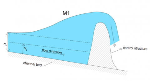
In this example, a triangular channel is considered with a mild slope of S0 =0.001, the Manning coefficient n=0.015, the discharge Q=4m3/s and the side slope Z=1.5. There is a control structure in the flow path of the channel that creates the GVF profile from the control structure site to upstream. The water depth in the control structure site is 2m.
Figure 1 shows a schematic view of the GVF profile in this channel.
Figure 1. The schematic view of the GVF profile in the channel with the mild slope (M1 profile in the open channel hydraulic)
As seen in Figure 1, the water surface profile (or GVF profile) decreases from the control structure site to upstream of channel.
Now, the GVF profile in this channel can be obtained by substituting example parameters in Eq. (12).
It should be noted that the presented solutions (Eqs. 4, 5 and 12) are series solutions. Therefore, it is necessary to check their convergence in reaching to the answer for the number of used terms. Certainly, in the analytical solutions that are presented in the series forms, using the first few terms is enough to obtain the exact solution. The expressed numerical solution (FDM solution) is presented to determine how many terms of the presented series are needed for obtaining the exact solution. By determining the number of terms, a continuous solution can be created to obtain GVF profile in the triangular channels with Manning equation.
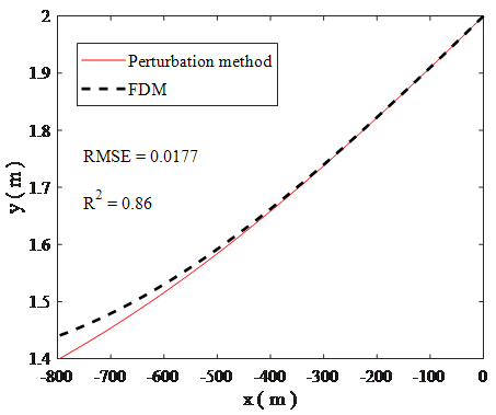
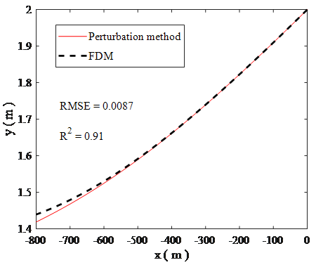
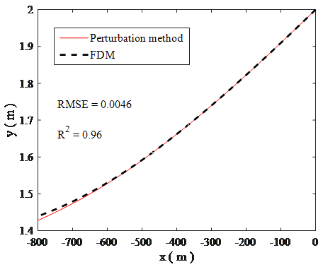
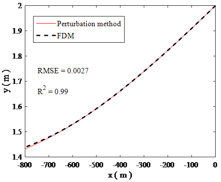
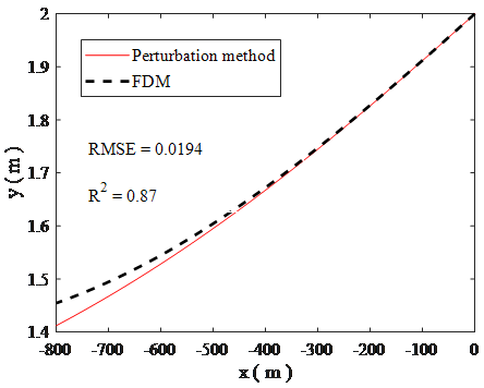
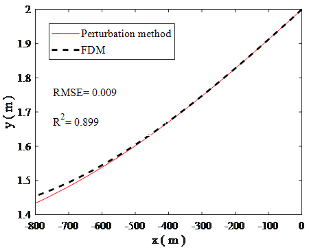
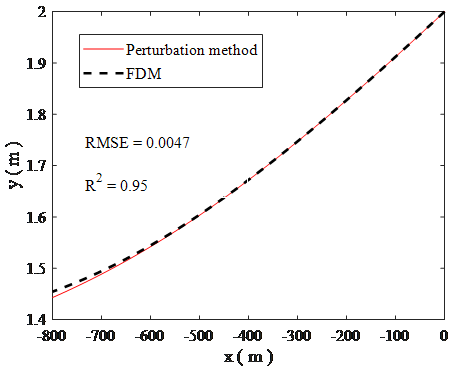
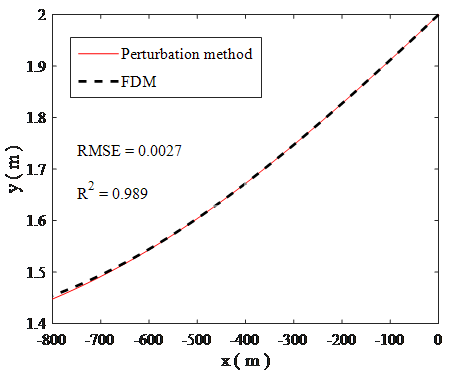
The GVF profile in this channel for different terms approximation of Eq. (12) are shown in Figure 2. It should be noted that in Figure 2, water surface profile draws from downstream to upstream of the channel flow.
As mentioned in defenition of Eq. (1), the distance along the channel (x) is positive in the direction of channel flow and therefore, When the profile is drawn from downstream to upstream of the channel (the opposite direction of the flow), the value of X is negative (horizental axes in Figures 2a to 2d) [34, 35]. Furthermore, the negative value for X is obtained from both numerical and analytical methods.
In this Figure, the first three terms approximation is equivalent to the sum of the first three terms and the corresponding constant (C** =C0+C1+C2) in Eq. (12). Also, the first four terms approximation means the sum of the first four terms and the corresponding constant (C** =C0+C1+C2+C3) in Eq. (12) and so on.
So that, Figures 2a, 2b, 2c and 2d are for the first three, four, five and six terms of Eq. (12), respectively.
As shown, by increasing the terms approximation of Eq. (12), GVF profile for the perturbation solution converges to the FDM profile (FDM is for Δx=1m). Therefore, as seen in Figure 2d, the perturbation profile is in excellent agreement with the FDM profile. Also, Errors as well as correlation among solutions are computed in terms of root mean squared error (RMSE) and absolute fraction of variance (R2) and shown in Figures 2a to 2d. R2 and RMSE parameters are computed as:
$R^{2}=1-\frac{\sum_{i=1}^{n}\left(y_{P M}-y_{F D M}\right)^{2}}{\sum_{i=1}^{n}\left(y_{P M}\right)^{2}}$
$R M S E=\sqrt{\frac{1}{n} \sum_{i=1}^{n}\left(y_{P M}-y_{F D M}\right)^{2}}$
where, yPM and yFDM are the water depth values by PM and FDM, respectively. Closer values of R2 to 1 and closer values of RMSE to 0, indicate good agreements between PM and FDM results. As shown in Figures, maximum value of R2 and minimum value of RMSE are in Figure 2d with six terms approximation. In other words, R2 value is closer to 1 and RMSE value is closer to zero by increasing the terms approximation.
Table 1 shows the water depth values at different distances for various terms approximation. As seen, difference in water depth is negligible at six terms approximation, and yPM is almost identical to yFDM at all distances. Relative error (RE) values in the Table are defined as:
Relative Error $(\mathrm{RE})=\left|\frac{y_{P M}-y_{F D M}}{y_{P M}}\right| \times 100 \%$
As shown, RE’s are all less than 0.5% which is deemed reasonable, and hence, it is concluded that convergence in Eq. (12) is very rapid.
According to the results, the PM can be applied to plot the water surface profile for the prismatic triangular channel when the Manning equation is utilized for the resistance equation.
(a) First three terms
(b) First four terms
(c) First five terms
(d) First six terms
Figure 2. GVF profiles in the triangular channel for various terms approximation in Eq. (12): a) First three terms, b) First four terms, c) First five terms, d) First six terms
Table 1. Water depth values for perturbation solution with various terms approximation, FDM solution, and the relative error (RE) in the Manning equation case
|
X (m) |
yPM (m) by first three terms |
yPM (m) by first four terms |
yPM (m) by first five terms |
yPM (m) by first six terms |
yFDM (m) ∆x=1 m |
RE (%) |
|
-100 |
1.9095 |
1.9095 |
1.9095 |
1.9095 |
1.9099 |
0.02 |
|
-300 |
1.7380 |
1.7395 |
1.7395 |
1.7395 |
1.7399 |
0.02 |
|
-500 |
1.5840 |
1.5895 |
1.5910 |
1.5915 |
1.5920 |
0.03 |
|
-800 |
1.4002 |
1.4185 |
1.4280 |
1.4325 |
1.4394 |
0.48 |
In this section, the Chezy equation is used for the energy line slope (Sf) in the governing equation (Eq. (1)). Therefore, Sf with the Chezy equation for the triangular channel is:
$S_{f}=\frac{Q^{2}}{\left(Z y^{2}\right)^{2} C^{2}\left(\frac{Z y}{2 \sqrt{1+Z^{2}}}\right)}=\frac{Q^{2}}{Z^{3} y^{5} C^{2} / 2 \sqrt{1+Z^{2}}}$ (13)
where, C is Chezy’s roughness coefficient. Here, the coefficient is assumed constant.
Now, Following the similar mathematical procedure as before (section 3), the answers for x0, x1, x2, … would be:
$x_{0}=\frac{1}{S_{0}}\left(y+\frac{Q^{2}}{2 g Z^{2} y^{4}}\right)+C_{0}^{*}$ (14a)
$x_{1}=\frac{2 Q^{2} \sqrt{\left(1+Z^{2}\right)}\left(\frac{2}{9} \frac{Q^{2}}{y^{9}}-\frac{1}{4} \frac{g Z^{2}}{y^{4}}\right)}{s_{0}^{2} \cdot Z^{5} \cdot C^{2} \cdot g}+C_{1}^{*}$ (14b)
$x_{2}=\frac{4 Q^{4} \cdot\left(1+Z^{2}\right)\left(\frac{1}{7} \frac{Q^{2}}{y^{14}}-\frac{1}{9} \frac{g Z^{2}}{y^{9}}\right)}{S_{0}^{3} \cdot Z^{8} \cdot C^{4} \cdot g}+C_{2}^{*}$ (14c)
$x_{3}=\frac{8 Q^{6} \cdot\left(1+Z^{2}\right)^{3 / 2}\left(\frac{2}{19} \frac{Q^{2}}{y^{19}}-\frac{1}{14} \frac{g Z^{2}}{y^{14}}\right)}{S_{0}^{4} \cdot Z^{11} \cdot C^{6} \cdot g}+C_{3}^{*}$ (14d)
$x_{4}=\frac{16 Q^{8} \cdot\left(1+Z^{2}\right)^{2}\left(\frac{1}{12} \frac{Q^{2}}{y^{24}}-\frac{1}{19} \frac{g Z^{2}}{y^{19}}\right)}{S_{0}^{5} \cdot Z^{14} \cdot C^{8} \cdot g}+C_{4}^{*}$ (14e)
$x_{5}=\frac{32 Q^{10} \cdot\left(1+Z^{2}\right)^{5 / 2}\left(\frac{2}{29} \frac{Q^{2}}{y^{29}}-\frac{1}{24} \frac{g Z^{2}}{y^{24}}\right)}{S_{0}^{6} \cdot Z^{17} \cdot C^{10} \cdot g}+C_{5}^{*}$ (14f)
where, C0*, C1*, C2*, C3*…are constants. The constants are obtained by boundary conditions (similar to Eqns. (10a), (10b), (10c) and etc.).
Finally, substituting Eqns. (14a), (14b), (14c) and etc. in Eq. (5) and applying some simplifications, the perturbation solution for the GVF profile, in this case, is written as:
$X=\left(\begin{array}{l}\sum_{m=0}^{\infty} \frac{2^{m} Q^{2 m}\left(1+Z^{2}\right)^{m / 2}}{S_{0}^{m+1} \cdot Z^{3 m+2} \cdot C^{2 m} \cdot g} \\ \times\left(\frac{2}{5 m+4} \frac{Q^{2}}{y^{5 m+4}}-\frac{1}{5 m-1} \frac{g Z^{2}}{y^{5 m-1}}\right)\end{array}\right)+C^{*}$ (15)
where, C* is C0*+C1*+C2*+···. Eq. (15) is the exact solution for the nonlinear governing equation (Eq. (1)) in the prismatic triangular channel. In order to confirm summations convergence in Eq. (15), water surface profile is calculated using summations truncation with different values of m in an applied example. The example parameters for this case are identical to those used in the previous section, except that the Chezy coefficient (C) is 60. As explained in the previous section, the presented solution (Eq. (15)) is series solution. Therefore, it is necessary to check its convergence in reaching to the answer for the number of used terms. By determining the number of terms, a continuous solution can be created to obtain GVF profile in the triangular channels with Chezy equation.
Figure 3 shows the GVF profile for summations truncation with different values of m in Eq. (15). So that, Figures 3a, 3b, 3c and 3d are for m=0~2, m=0~3, m=0~4 and m=0~5, respectively. As explained in the previous section, the X values are negative in the horizontal axes of Figures 3a to 3b.
(a) m=0~2
(b) m=0~3
(c) m=0~4
(d) m=0~5
Figure 3. GVF profiles in the triangular channel for summations truncation with a different value of m in Eq. (15): a) m=0~2, b) m=0~3, c) m=0~4, d) m=0~5
As seen, by increasing m values in Eq. (15), the perturbation profile is more consistent with the FDM profile (see R2 and RMSE values in Figures 3a to 3d). Thus, Figure 3d for m=0~5 shows an excellent agreement between them. In other words, R2 value is very close to 1 and RMSE value is very close to zero in m=0~5 or Figure 3d.
Also, Table 2 shows the water depth values at different distances for various m values. As seen, difference in water depth is negligible at m=0~5, and yPM is almost identical to yFDM at all distances. As seen, the maximum RE is 0.48% and therefore, yPM values are judged as having excellent agreements with yFDM.
According to the found results, the PM can be used to obtain the water surface profile for a prismatic triangular channel with mild slope (M1 profile in the open channel hydraulic) when the Chezy equation is utilized for the energy line slope.
Table 2. Water depth values for perturbation solution with various m values, FDM solution, and the relative error (RE) in the Chezy equation case
|
X(m) |
yPM (m) by m=0~2 |
yPM (m) by m=0~3 |
yPM (m) by m=0~4 |
yPM (m) by m=0~5 |
yFDM (m) ∆x=1 m |
RE (%) |
|
-100 |
1.9115 |
1.9120 |
1.9120 |
1.9120 |
1.9122 |
0.01 |
|
-300 |
1.7445 |
1.7465 |
1.7470 |
1.7470 |
1.7473 |
0.017 |
|
-500 |
1.5950 |
1.6010 |
1.6030 |
1.6040 |
1.6044 |
0.02 |
|
-800 |
1.4115 |
1.4335 |
1.4430 |
1.4475 |
1.4545 |
0.48 |
In the current study, semi-analytical solutions have been presented by the Perturbation Method (PM) for solving the GVF equation in a prismatic triangular channel. Two cases were investigated in this paper. In case 1, the Manning equation and in case 2, the Chezy equation were applied as the resistance equations. Semi-analytical profiles in two cases were compared to the Finite Difference Method (FDM) profiles. Also, the effect of the terms approximation and the summations truncation in the PM was investigated for these cases. By determining the number of terms, a continuous solution can be created to obtain GVF profile in the triangular channels.
The results have shown that by increasing the terms approximation in the PM, GVF profiles coincide with FDM profiles. These semi-analytical solutions may be used as a benchmark solution for verification and efficiency assessment of other numerical techniques.
Furthermore, the proposed method in this paper can be used as a new idea in providing semi-analytical solutions to other open channel works such as the spatially varied flow equation. Investigation of analytical solutions for trapezoidal, circular, parabolic and non-prismatic channels using PM is suggested for future researches in this field.
|
Fr |
Froude number |
|
S0 |
The longitudinal slope of the channel |
|
Sf |
Energy line slope |
|
T |
Width of the water surface, m |
|
A |
Cross section area of the channel flow, m2 |
|
Q |
Discharge, m3/s |
|
g |
Acceleration of gravitation, m.s-2 |
|
Z |
Side slope of the triangular channel |
|
R |
The hydraulic radius of triangular channel, m |
|
n |
Manning roughness coefficient |
|
x |
The distance along the channel, m |
|
C |
Chezy’s roughness coefficient |
[1] Zaghloul, N.A., Anwar, M.N. (1991). Numerical integration of gradually varied flow in trapezoidal channel. Computer Methods in Applied Mechanics and Engineering, 88(2): 259-272. http://dx.doi.org/10.1016/0045-7825(91)90258-8
[2] Rhodes, D.G. (1998). Gradually varied flow solution in Newton-Raphson form. Journal of Irrigation and Drainage Engineering, 124(4): 233-235. http://dx.doi.org/10.1061/(ASCE)07339437(1998)124:4(233)
[3] Dey, S. (2000). Chebyshev solution as aid in computing GVF by standard step method. Journal of Irrigation and Drainage Engineering, 126(4): 271-274. http://dx.doi.org/10.1061/(ASCE)07339437(2000)126:4(271)
[4] Sen, D.J., Garg, N.K. (2002). Efficient algorithm for gradually varied flows in channel networks. Journal of Irrigation and Drainage Engineering, 128(6): 351-357. http://dx.doi.org/10.1061/(ASCE)07339437
[5] Reddy, H.P., Bhallamudi, S.M. (2004). Gradually varied flow computation in cyclic looped channel networks. Journal of Irrigation and Drainage Engineering, 130(5): 424-431. http://dx.doi.org/10.1061/(ASCE)07339437(2004)130:5(424)
[6] Islam, A., Raghuwanshi, N.S., Singh, R., Sen, D.J. (2005). Comparison of gradually varied flow computation algorithms for open-channel network. Journal of Irrigation and Drainage Engineering, 131(5): 457-465. http://dx.doi.org/10.1061/(ASCE)0733-9437(2005)131:5(457)
[7] Nabila, C.K., Azzedine, S. (2019). Numerical study of surface roughness effects on the behavior of fluid flow in micro-channels. Mathematical Modelling of Engineering Problems, 6(2): 285-292. https://doi.org/10.18280/mmep.060217
[8] Kaya, B. (2011). Investigation of gradually varied flows using differential quadrature method. Scientific Research and Essays, 6(13): 2630-2638. https://doi.org/10.5897/SRE10.827
[9] Kurnatowski, J. (2011). Comparison of analytical and numerical solutions for steady gradually varied open-channel flow. Polish Journal of Environmental Studies, 20(4): 925-930.
[10] Menni, Y., Chamkha, A.J., Zidani, C., Benyoucef, B. (2019). Numerical analysis of heat and nano fluid mass transfer in a channel with detached and atached baffle plates. Mathematical Modelling of Engineering Problems, 6(1): 52-60. https://doi.org/10.18280/mmep.060107
[11] Artichowicz, W., Szymkiewicz, R. (2014). Computational issues of solving the 1D steady gradually varied flow equation. Journal of Hydrology and Hydromechanics, 62(3): 226-233. http://dx.doi.org/10.2478/johh-2014-0031
[12] Reddy, H.P., Chaudhry, M.H., Imran, J. (2014). Computation of gradually varied flow in compound open channel networks. Sadhana, 39(6): 1523-1545. https://doi.org/10.1007/s12046-014-0299-5
[13] Ghazizadeh, S., Abedini, M.J. (2017). Gradually Varied Flow modeling: How to choose a reach with maximum information content? Flow Measurement and Instrumentation, 56: 56-60. http://dx.doi.org/10.1016/j.flowmeasinst.2017.05.001
[14] Malekabadi, M.J., Kalateh, F. (2019). Gradually varied flow profile based on adaptive pattern. ISH Journal of Hydraulic Engineering, 25(2): 223-231. https://doi.org/10.1080/09715010.2017.1408035
[15] Artichowicz, W., Gąsiorowski, D. (2018). Numerical Analysis of Steady Gradually Varied Flow in Open Channel Networks with Hydraulic Structures. In Free Surface Flows and Transport Processes, Springer, Cham, 127-142. https://doi.org/10.1007/978-3-319-70914-7_6
[16] Sivapragasam, C., Saravanan, P., Ganeshmoorthy, K., Muhil, A., Dilip, S., Saivishnu, S. (2019). Mathematical Modeling of Gradually Varied Flow with Genetic Programming: A Lab-Scale Application. Information and Communication Technology for Intelligent Systems, Smart Innovation, Systems and Technologies, 106. https://doi.org/10.1007/978-981-13-1742-2_40
[17] Zarif Sanayei, H.R., Rakhshandehroo, G.R., Talebbeydokhti, N. (2016). New analytical solutions to 2-D water infiltration and imbibition into unsaturated soils for various boundary and initial conditions. Iranian Journal of Science and technology, Transaction of Civil Engineering, 40(3): 219-239. https://doi.org/10.1007/s40996-016-0018-z
[18] Zarif Sanayei, H.R., Rakhshandehroo, G.R., Talebbeydokhti, N. (2019). Analytical solutions for water infiltration into unsaturated–semi-saturated soils under different water content distributions on the top boundary. Iranian Journal of Science and Technology, Transaction of Civil Engineering, 1-14. https://doi.org/10.1007/s40996-019-00245-3
[19] Patil, R.G., Diwanji, V.N., Khatsuria, R.M. (2001). Integrating equation of gradually varied flow. Journal of Hydraulic Engineering, 127(7): 624-625. http://dx.doi.org/10.1061/(ASCE)07339429(2001)127:7(624)
[20] Vatankhah, A.R. (2010). Analytical integration of the equation of gradually varied flow for triangular channels. Flow Measurement and Instrument, 21(4): 546-549. https://doi.org/10.1016/j.flowmeasinst.2010.09.004
[21] Jan, C.D., Chen, C.L. (2013). Gradually-varied open-channel flow profiles normalized by critical depth and analytically solved by using Gaussian hypergeometric functions. Hydrology & Earth System Sciences Discussions, 17(3): 973-987. http://dx.doi.org/10.5194/hess-17-973-2013
[22] Vatankhah, A.R. (2015). Analytical solution of gradually varied flow equation in circular channels using variable manning coefficient. Journal of Flow Measurement and Instrumentation, 43: 53-58. https://doi.org/10.1016/j.flowmeasinst.2015.04.004
[23] Tajari, M., Dehghani, A.A., Meftah Halaghi, M. (2018). Semi analytical solution and numerical simulation of water surface profile along duckbill weir. ISH Journal of Hydraulic Engineering, 1-8. https://doi.org/10.1080/09715010.2018.1515042
[24] Homayoon, L., Abedini, M.J. (2019). Development of an analytical benchmark solution to assess various gradually varied flow computations. ISH Journal of Hydraulic Engineering, 1-9. https://doi.org/10.1080/09715010.2018.1563872
[25] Swamee, P.K. (2003). Length of gradually varied flow profiles. ISH Journal of Hydraulic Engineering, 9(2): 70-79. https://doi.org/10.1080/09715010.2003.10514734
[26] Venutelli, M. (2004). Direct integration of the equation of gradually varied flow. Journal of Irrigation and Drainage Engineering, 130(1): 88-91. https://doi.org/10.1061/(ASCE)07339437(2004)130:1(88)
[27] Vatankhah, A.R. (2010). Exact sensitivity equation for one-dimensional steady-state shallow water flow (Application to model calibration). Journal of Hydrologic Engineering, 15(11): 939-945. https://doi.org/10.1061/(ASCE)HE.1943-5584.0000272
[28] Vatankhah A.R., Easa S.M. (2011). Direction integration of manning based GVF flow equation. In Proceedings of the Institution of Civil Engineers-Water Management. Thomas Telford Ltd. Water Manage ICE, 164(5): 257-264. https://doi.org/10.1680/wama.2011.164.5.257
[29] Vatankhah, A.R. (2011). Direct integration of gradually varied flow equation in parabolic channels. Flow Measurement and Instrumentation, 22(3): 235-241. https://doi.org/10.1016/j.flowmeasinst.2011.03.003
[30] Jan, C.D., Chen, C.L. (2012). Use of the gaussian hypergeometric function to solve the equation of gradually-varied flow. Journal of Hydrology, 456: 139-145. https://doi.org/10.1016/j.jhydrol.2012.06.023
[31] Vatankhah, A.R. (2011). Direct integration of manning-based GVF equation in trapezoidal channels. Journal of Hydrologic Engineering, 17(3): 455-462. https://doi.org/10.1061/(ASCE)HE.1943-5584.0000460
[32] Vatankhah, A.R., Easa, S.M. (2014). Briefing: Direct solution for water surface profile in circular channels. Proceedings of the Institution of Civil Engineers-Water Management, 167(6): 311-317. http://dx.doi.org/10.1680/wama.12.00119
[33] Vatankhah, A.R., Easa, S.M. (2013). Accurate gradually varied flow model for water surface profile in circular channels. Ain Shams Engineering Journal, 4(4): 625-632. https://doi.org/10.1016/j.asej.2013.01.005
[34] Chaudhry, M.H. (2007). Open-channel flow. Springer Science & Business Media. http://dx.doi.org/10.1007/978-0-387-68648-6
[35] Szymkiewicz, R. (2010). Numerical modeling in open channel hydraulics. Springer Science & Business Media, 83. http://dx.doi.org/10.1007/978-90-481-3674-2
[36] Hermann, M., Saravi, M. (2016). Nonlinear ordinary differential equations. Springer India. http://dx.doi.org/10.1007/978-81-322-2812-7