Komaravolu V.B. Rajakumar* | Venkata S.R. Pavan Kumar Rayaprolu | Kuppareddy S. Balamurugan | Vedagiri Bharat Kumar
© 2020 IIETA. This article is published by IIETA and is licensed under the CC BY 4.0 license (http://creativecommons.org/licenses/by/4.0/).
OPEN ACCESS
Current examination concern with influence of radiation absorption and viscous dissipation on MHD free convective flow of Casson fluid model past a semi-infinite vertical porous plate. Multiple regular perturbation law was utilized for solving non-dimensional governing equations. Computations are performed graphically to scrutinize the deportment of fluid velocity, temperature and concentration. And also skin friction, nusselt number and sherwood number are illustrated in tabular form on the vertical porous plate with the dissimilarity of emerging physical parameters. Finally, conclude that the enhancement of Eckert number leads to rise in velocity, but contrast repercussions were demonstrated in case of temperature. And also sherwood number declined with the rise in chemical reaction as well as schmidt number. However, velocity and temperature were diminishned with amplify of Casson fluid and thermal radiation parameters.
radiation absorption, viscous dissipation, MHD, chemical reaction, heat generation, Casson fluid, porous medium multiple regular perturbation law
Non-Newtonian fluid flow arises in a plenty of divisiveness of chemical as well as material processing engineering. There are heterogeneous categorizations of non-Newton fluids analogous Williamson fluid, couple stress fluid, power law fluid, viscoelastic fluid, Prandtl-Eyring fluid, microplar fluid and so on. So too with these, there is one more non-Newtonian fluid model is consciousness as the Casson fluid model. It is one of the pseudo plastic fluids this fluid was pioneered by Casson. The Casson fluid model is indistinguishable to a non-Newtonian fluid which does not emulate the Newtonian relationship between the shear stress as well as shear rate and also it discloses the characteristics of yield stress. In addition, Casson fluid acts like a material in nature that deforms continually beneath applied shear stress. These non-Newtonian fluids have non-linear relationship between shear stress and shear strain. This has noteworthy applications in biomechanics and polymer processing industries. The examples of Casson fluid are Aloe era juices, Jelly, pasta sauce, honey, soup, focused fruit juices, blood and polymer solutions. Human blood conjointly treated as Casson fluid. Several researchers are demonstrated emerging fascinate on Casson fluid model and elucidated various condition, such as Harshad et al. [1], Kataria et al. [2] & Biswas et al. [3].
The investigation of Magneto Hydrodynamic (MHD) flow of non-Newtonian fluid in a porous medium has attracted the attentions of a various researchers. Obviously, it is owing to the reality that such phenomenon’s are predominantly establish in the optimization of solidification processes of metals and metal alloys, the geothermal sources examination and nuclear fuel debris treatment. However, non-Newtonian fluids are slight compare to Newtonian fluids. Certainly, the resulting equations of non-Newtonian fluids give highly non-linear differential equations which are generally difficult to solve. These equations add further complexities when MHD flows in a porous space have been taken into account. Sufficient applications for the MHD flows of Casson fluids in a porous medium are experienced in biological systems, irrigation problems, process of petroleum, heat-storage beds, textile, polymer composite and paper industries. Several researchers have been presented on different aspects of MHD flows of Casson fluid flows passing through a porous medium. Various examinations have been introduced on different parts of MHD non-Newtonian liquid streams going through a permeable medium. Srinivasa Raju et al. [4] have discussed significance of Casson fluid model and influence of dissipative on unsteady MHD natural convection flow over on a vertical surface along with constant heat flux in presence of angle of inclination as well as chemical reaction. The outcomes obtained in this investigation was conclude that the enhancement of dissimilar parameter of chemical reaction, angle of inclination, Schmidt number and Prandtl number leads to diminished in velocity. But reverse effect was occurred in case of Eckert as well as Soret numbers. The enhancement of different values of Eckert number leads to rise in temperature, but inverse effect was happened in case of Prandtl number. Khalid et al. [5] have examined Casson fluid model on unsteady MHD flow of a past an oscillating vertical permeable plate by means of constant wall temperature. Jithender Reddy et al. [6] have investigated significance of Casson fluid model on MHD free convection flow of an oscillating vertical permeable plate in the presence viscous dissipation. In this examination it was culminate that the results indicate the enhancement of dissimilar values of Eckert number given results rise in the velocity as well as temperature profile. But inverse effect was occurred in case of skin-friction and Nusselt number. Hari et al. [7] discussed Casson fluid model on unsteady MHD free convective flow past an oscillating non-parallel permeable plate in the influence of uniform transverse magnetic field and thermal radiation. In this examination isothermal as well as sloped wall temperatures were considered. Rammohan Reddy et al. [8] have explored MHD visco-elastic and radiative free convective flow of an incompressible, chemically, electrically conducting and rotating fluid through a porous medium filled in a vertical channel within the view of thermal diffusion. The ODE’s are solved by utilizing perturbation technique. Mohamed Abd El-Aziz [9] have examined the influence heat transfer on unsteady MHD boundary layer Casson fluid flow with thin liquid film over a stretched sheet in presence of thermal radiation and dissipation. From this paper it was observed that the heat transfer rate lessens with rise in thermal conductivity parameter as well as Eckert number. Further, the inverse impact was found with an expansion in radiation parameter. Srinivasa Raju et al. [10] have discussed significance of double diffusion and DuFour effect on unsteady MHD free-convection, incompressible, electrically conducting, flow on an electrically conducting, viscous fluid flow past a semi-infinite inclined vertical permeable plate moving with a uniform velocity in presence of chemical reaction as well as thermal radiation.
In the flow of fluids, mechanical energy is degraded into heat and this process is called viscous dissipation. The viscous dissipation effects are imperative in geophysical flows and in certain industrial operations. It was usually characterized by the Eckert number (Ec). In the literature, extensive research work is available to examine the effect of free convective Casson fluid flow past a porous plate. Srinivasa Raju et al. [11] have analyzed Casson fluid model as well as viscous dissipative effects on unsteady MHD natural convection flow over an inclined plate in presence of magnetic field as well as heat and mass transfer. Saidulu et al. [12] investigated the significance of Casson fluid model on MHD free connective boundary layer flow of heat transfer as regards porous medium, an exponentially stretching sheet with fluid velocity slip as well as thermal slip conditions in the presence of heat source. Pushpalatha et al. [13] studied unsteady MHD free convection flow of a Casson fluid enclosed by a moving vertical flat plate in a rotating system with convective boundary conditions. Vajravelu et al. [14] examined numerically the significance of heat transfer in the laminar, incompressible boundary layer flow of a viscous fluid over a continuous surface, linearly stretching in existence of variable wall temperature subject to suction. In this paper frictional heating effect as well as internal heat absorption has been considered. According to exploration it was ascertained that the surface with proscribed surface temperature and the surface with proscribed wall heat flux have been taken into consideration. Suresh et al. [15] have studied numerically influence of viscous dissipation, internal heat generation as well as thermal radiation in presence of variable thermal conductivity. Venkateswarlu et al. [16] have analyzed the influence of viscous dissipation and chemical reaction on MHD natural convective flow of a Casson fluid past a stretched sheet in the existence of Soret, Dufour and variable thermal conductivity. Qasim Muhammad et al. [17] have considered the influence of viscous dissipation on MHD free convective Blasius flow in a Casson fluid model with convective boundary conditions.
The influence of radiation and chemical reaction on MHD free convective flow of double diffusion problems have turned out to be salient in technical world. A few engineering processes eventuate at high temperatures and henceforth the influence of thermal radiation heat transfer is indispensable for outlining of appropriate types of gear, for example, distinctive propulsion devices for airplane, atomic power plants, gas turbines, rockets and satellites. At the point when radiative heat transfer eventuates in the electrically conducting fluid, it is ionized because of the high operational temperature. In point of view of these, a lot of researchers have made commitments to the examination of fluid flow by means of thermal radiation. Investigation of a chemical reaction in MHD free convection flow with double diffusion problems are salient for chemical industries owing to its massive applications in numerous fields of science as well as engineering, such as in manufacturing of ceramics, evaporation, drying, reservoir engineering and food processing. The sort of chemical reaction depends on a lot of factors, for example foreign mass, active fluid and stretching of sheet and so on. Venkateswarlu et al. [18] examined numerically, the influence of radiation absorption on MHD free convective Casson fluid flow over a semi-infinite vertical permeable plate by means of chemical reaction and viscous dissipation. The non-Newtonian fluid behaviour is considered by using the Casson fluid model. In this scrutiny it was perceived that the dimensionless coupled non-linear PDE’s are solved by utilizing very economical and simple method multiple regular perturbation. Harinath Reddy et al. [19] have contemplated the significance of Casson fluid model on unsteady MHD free convective flow double diffusion past an oscillating vertical plate entrenched in a porous medium in the influence of radiation absorption and chemical reaction with constant wall temperature and concentration flow. Bala Anki Reddy [20] have assessed theoretically, steady 2D MHD free convective Casson fluid flow of over an exponentially inclined permeable stretched surface in the effect of chemical reaction and thermal radiation. Here Solutal slip, Velocity slip and thermal slip is taken in to consideration. In this investigation it was conclude that the energy boundary layer thickness reduced by means of rise in the Casson fluid parameter. In addition, the incremental values of thermal radiation as well as Prandtl number leads to rise in fluid temperature. Imran Ullah [21] have considered significance of Casson fluid model and thermal radiation on unsteady MHD mixed convection flow over a stretching sheet embedded in a porous medium along with magnetic field as well as chemical reaction. Eswara Rao et al. [22] have reported thermal radiation, viscous dissipation and chemical reaction effects on MHD natural convective Casson fluid flow over an exponentially inclined permeable stretching surface. Mythili et al. [23] & Jasmine Benazir et al. [24] studied importance of Casson fluid model and heat generating or absorbing as well as chemically reacting flow over a vertical cone along with horizontal plate saturated with non-Darcy porous medium in presence of Soret as well as DuFour effects. In this examination it was observed that a numerical computation for the non-linear couple partial differential equations are solved by employing implicit finite the Crank–Nicolson difference method. Rajakumar et al. [25] investigated analytically the influence of chemical reaction and viscous dissipation on MHD free convective flow past a semi-infinite moving vertical permeable plate with radiation absorption. Ramaiah et al. [26] reported influence of viscoelastic fluid and radiation absorption on MHD free convective flow of in the course of porous medium surrounded by an oscillating porous plate in the presence of heat source and chemical reaction. Rajakumar et al. [27] have illustrated influence of viscous dissipation on MHD free convective flow through a semi-infinite moving vertical permeable plate in presence of heat generation and radiation absorption and chemical reaction in presence of variable section. Rajakumar et al. [28] have explored influence of Dufour, radiation absorption, chemical reaction, and viscous dissipation on unsteady MHD free convective Casson fluid flow through a semi-infinite vertical oscillatory porous plate of time dependent permeability with Hall and ion-slip current in a rotating system.
In this paper the effects of chemical reaction and radiation absorption on MHD free convection flow of Casson fluid past a semi-infinite moving vertical porous plate with viscous dissipation has been investigated. The flow was unsteady and constrained to the laminar domain. The governing equations for this consideration are solved utilizing multiple-regular perturbation method. The effects of diverse physical parameters on temperature, concentration and velocity, fields are plotted graphically. With the help of these, the skin friction, Nusselt number and Sherwood number was shown in the tabular form.
In this problem, consider the effects of viscous dissipation and radiation absorption on unsteady two dimensional MHD free convective Casson fluid flow of a viscous, incompressible fluid over a vertical porous plate by means of heat and mass transfer in a uniform of a pressure grading. The following assumptions are listed below:
The rheological equation of state for the Cauchy stress tensor of Casson fluid can be written as
τ=τ0+μα∗ (1)
Equivalently τij={2[μB+py√2π]eijπ>πc2[μB+py√2πc]eijπ<πc (2)
⇒π=eijeij (3)
eij= the (i,j)th component of deformation rate, τ0 = Casson yield stress, π = the product based on the non-Newtonian fluid, πc =a critical value of this product, μB = plastic dynamic viscosity of the non-Newtonian fluid, μ = the dynamic velocity, α∗ = shear rate.
The yield stress of fluid =py=μB√2πγ (4)
Some fluids require a gradually increasing shear stress to maintain a constant strain rate and are called Rheopectic, in the case of Casson fluid
Flow where τ>τc,μ=μB+py√2π (5)
The Kinematic velocity v=μρ=μBρ[1+1γ] (6)
Finally. the Casson fluid parameter is γ=μB√2πcpy (7)
Let the ˉx -axis be taken along the porous plate in the vertical direction and ˉy -axis in the direction of perpendicular to the flow. Let ˉx and ˉy are the dimensional distance along the perpendicular to the plate and τ1 is the dimensional time. ˉu and ˉv are the components of dimensional velocities along ˉx and ˉy directions. Suppose that transverse magnetic field of the uniform strength is to be applied normal to the plate. The radiate heat flux in the ˉx - direction is considered insignificant in comparison with that in ˉy - direction. Physical model of the problem has been shown in Figure 1. It is supposed that voltage is not applied which implies the nonappearance of an electric field. Induced magnetic field is supposed to be insignificant. C* and g* are the dimensional concentration and acceleration owing to gravity, Q0(T∗−T∗∞) is the amount of heat generated per unit volume. Q0 is the constant where either Q0<0 or Q0>0 , g is acceleration owing to gravity. gβ(T∗−T∗∞) is the body force owing to non-uniform temperature, gβ∗(C∗−C∗∞) is the body force owing to non-uniform concentration. Viscous dissipation, Radiation absorption and permeability of porous medium are taken into account. The fluid contains constant thermal conductivity and kinematic viscosity, the Boussinesqu’s approximation has been considered for the flow. The homogeneous chemical reaction is of first order with rate constant between the diffusing species and the fluid is considered.
Figure 1. Physical model of the problem
From the above assumptions, the unsteady flow is governed by the following partial differential equations.
Equation of continuity:
∂ˉv∂ˉy=0 (8)
Equation of Momentum:
∂¯u∂τ1+¯v∂¯u∂→y=−1ρ∂¯p∂¯x+ϑ(1+1γ)∂2¯u∂¯y2+gβ(¯T−¯T∞)+g¯β(¯C−¯C∞)−ϑ¯K¯u−σρB20¯u} (9)
∂ˉT∂τ1+ˉv∂ˉT∂ˉy=KρCp∂2ˉT∂ˉy2+Q0ρCp(ˉT−¯T∞)−1KρCp∂ˉqr∂ˉy+ϑCp(1+1γ)(∂ˉu∂ˉy)2+ˉR(ˉC−¯C∞)} (10)
Equation of Concentration:
∂ˉC∂τ+ˉv∂ˉC∂ˉy=D∂2ˉC∂ˉy2−Kr(ˉC−¯C∞) (11)
The boundary conditions for velocity, temperature and concentration field are given by
ˉu=0,ˉT=¯Tw+εeˉnτ(¯Tw−¯T∞),ˉC=¯Cw+εeˉm(¯Cw−¯C∞) at ˉy=0ˉu=U0(1+εeˉnτ),ˉT→ˉT∞,ˉC→¯C∞Asˉy→∞} (12)
From the equation of the continuity it is obvious that the suction velocity at the plate surface is a function of time only and we shall take it in the form:
¯v=−v0(1+εAe¯nτ) (13)
From the equation of momentum equation gives
−1ρ∂¯p∂¯x=d¯U∞dτ+ϑ¯K¯U∞+σρB20¯U∞ (14)
Eliminating −1ρ∂¯p∂¯x in the Eq. (9) by using (14) then we get
∂ˉu∂τ+ˉv∂ˉu∂y=dˉU∞dt+ϑ(1+1γ)∂2ˉu∂ˉy2+gβ(ˉT−ˉT∞)+gˉβ(ˉC−ˉC∞)+ϑK(¯U∞−ˉu)+σρB20(¯U∞−ˉu)} (15)
The radiative heat flux term by using the Rosseland approximation is given by
¯qr=−4¯σS3¯ke∂¯T4∂¯y (16)
We assume that the temperature difference within the flow is sufficiently small such that ¯T4 can be expressed as a linear function of the temperature; this is expanding in Taylor series about ¯T∞ and neglecting higher order terms to give:
¯T≅4¯T¯T3∞−3¯T∞ (17)
By using Eqns. (16) and (17) into equation of energy (10) can be changed into following form:
∂ˉT∂τ+v∂ˉT∂y=KρCp∂2ˉT∂ˉy2+Q0ρCp(ˉT−¯T∞)+16σST−3∞3ρCpke∂2ˉT∂ˉy−2+ϑCp(1+1γ)(∂ˉu∂ˉy)2+ˉR(ˉC−¯C∞)} (18)
Now Non-dimensional quantities are defined as
f=¯uU0,v=¯vV0,U∞=¯U∞U0,y=V0¯yϑ,Up=¯upU0t=V20τ1ϑ,¯K=Kϑ2V20,¯T=¯T∞+θ(¯Tw−¯T∞),¯n=V20nϑ¯C=¯C∞+C(¯Cw−¯C∞)} (19)
After substituting the boundary conditions and non-dimensional variables in the governing Eqns. (11), (15) and (18) and taking into account Eq. (13) then we get
∂f∂t−(1+ϵAent)∂f∂y=dU∞dt+(1+1γ)∂2f∂y2+Grθ+GmC+ϕ(U∞−U)} (20)
∂θ∂t−(1+∈Aent)∂θ∂y=(Pr (21)
\frac{\partial C}{\partial t}-\left( 1+\in A{{e}^{nt}} \right)\frac{\partial C}{\partial y}={{\left( Sc \right)}^{-1}}\frac{{{\partial }^{2}}C}{\partial {{y}^{2}}}-Kr\,\,\,C (22)
Boundary conditions (12) are given by the following form
\left.\begin{array}{l} f=0, \theta=1+\varepsilon e^{n t}, C=1+\varepsilon e^{n t} \quad A t y=0 \\ f=U_{\infty}=\left(1+\varepsilon e^{n t}\right), \theta \rightarrow 0, C \rightarrow 0 \quad A s y \rightarrow \infty \end{array}\right\} (23)
\left.\begin{array}{l} G r=\frac{\vartheta \beta g\left(\bar{T}_{w}-\bar{T}_{\infty}\right)}{V_{0}^{2} U_{0}}, G m=\frac{\vartheta \beta^{*} g\left(\bar{C}_{w}-\bar{C}_{\infty}\right)}{V_{0}^{2} U_{0}}, M=\frac{\sigma B_{0}^{2}}{\rho V_{0}^{2}} \\ \eta=\frac{\vartheta Q_{0}}{\rho V_{0}^{2} C_{P}}, \phi=M+\frac{1}{K} \operatorname{Pr}=\frac{\rho \vartheta C_{p}}{k} E c=\frac{U_{0}^{2}}{C_{p}\left(\bar{T}_{w}-\bar{T}_{\infty}\right)} \\ R=\frac{4 \sigma \bar{T}_{\infty}^{-3}}{k_{e} k}, S c=\frac{\vartheta}{D}, R a=\frac{\bar{R} \vartheta\left(\bar{C}_{w}-\bar{C}_{\infty}\right)}{V_{0}^{2}\left(\bar{T}_{w}-\bar{T}_{\infty}\right)}, K r=\frac{k_{1} \vartheta}{V_{0}^{2}} \end{array}\right\} (24)
The problem posted in Eqns. (20), (21) and (22) subject to the boundary conditions presented in Eq. (23) it has been explored numerically through Multiple Regular Perturbation law. This is more economical and flexible from analytical point of view. The behaviors of velocity, temperature, concentration, Skin-friction, Nusselt number and Sherwood numbers has been discussed in detail for variation of thermo physical parameters. The solution is assumed to be as,
\left.\begin{array}{l} f=f_{0}(y)+\varepsilon e^{n t} f_{1}(y) \\ \theta=\theta_{0}(y)+\varepsilon e^{n t} \theta_{1}(y) \\ C=C_{0}(y)+\varepsilon e^{n t} C_{1}(y) \end{array}\right\} (25)
Substituting Eq. (25) in Eqns. (20), (21) and (22) then we get the subsequent pairs of equations for (f0, θ0, C0) & (f1, θ1, C1)
\left( 1+\frac{1}{\gamma } \right)f_{0}^{''}+f_{0}^{'}-N{{f}_{0}}=-\phi -Gr\,\,{{\theta }_{0}}-Gm\,\,{{C}_{0}} (26)
\left.\begin{array}{r} \left(1+\frac{1}{\gamma}\right) f_{1}^{\prime \prime}+f_{1}^{\prime}-(N+n) f_{1}=-(\phi+n)-A f_{0}^{\prime}-G r \theta_{1} \\ -G m C_{1} \end{array}\right\} (27)
\left.\begin{array}{rl} (3+4 R) \theta_{1}^{\prime \prime}+3 \operatorname{Pr} \theta_{1}^{\prime}-3 \operatorname{Pr}(n-\eta) \theta_{1}=-3 \operatorname{Pr} A \theta_{0}^{\prime} \\ -6 E c\left(1+\frac{1}{\gamma}\right) P_{r} f_{0}^{\prime} f_{1}^{\prime}-3 \operatorname{Pr} R a C_{1} \end{array}\right\} (28)
\left.\begin{array}{r} (3+4 R) \theta_{0}^{\prime \prime}+3 \operatorname{Pr} \theta_{0}^{\prime}+3 \operatorname{Pr} \eta \theta_{0}=-3 \operatorname{Pr} E c\left(1+\frac{1}{\gamma}\right)\left(f_{0}^{\prime}\right)^{2} \\ -3 \operatorname{Pr} R a C_{0} \end{array}\right\} (29)
C_{0}^{''}+Sc\,\,C_{0}^{'}-Sc\,\,Kr\,\,{{C}_{0}}=0 (30)
C_{1}^{''}+Sc\,C_{1}^{'}-Sc\,\,\,\left( Kr+n \right){{C}_{1}}=-Sc\,\,AC_{0}^{'} (31)
The corresponding boundary conditions can be written as
\begin{aligned} f_{0} &=0, f_{1}=0 \theta_{0}=1, \theta_{1}=1, C_{0}=1 C_{1}=1, \text { at } y=0 \\ f_{0}=1, f_{1} &=1, \theta_{0} \rightarrow 0, \theta_{1} \rightarrow 0, C_{0} \rightarrow 0, C_{1} \rightarrow 0 \text { as } y \rightarrow \infty \end{aligned} (32)
Here Eqns. (26) to (31) are still coupled and non-linear, whose exact solutions are not possible. So we expand {{f}_{0}},\ {{f}_{1}}\ {{\theta }_{0}}\ {{\theta }_{1}} . Initialy we solve equation (30) and equation (31) by using Eq. (32) then we get
{{C}_{0}}={{e}^{-{{X}_{1}}y}} (33)
{{C}_{1}}={{e}^{-{{X}_{2}}y}}\left( 1-{{h}_{1}} \right)+{{e}^{-{{X}_{1}}y}}{{h}_{1}} (34)
Now utilizing multi parameter perturbation law and presumptuous E c<<1.
\left.\begin{array}{l} f_{0}=f_{00}+E c f_{01}+0(\varepsilon)^{2} \ldots \ldots \ldots . \\ \theta_{0}=\theta_{00}+E c \theta_{01}+0(\varepsilon)^{2} \ldots \ldots \ldots . \\ f_{1}=f_{10}+E c f_{11}+0(\varepsilon)^{2} \ldots \ldots \ldots \ldots . \\ \theta_{1}=\theta_{10}+E c \theta_{11}+0(\varepsilon)^{2} \ldots \ldots \ldots \ldots . \end{array}\right\} (35)
By utilizing Eq. (35) in Eqns. (26) to (29) we get the subsequent set of differential equation
\left( 1+\frac{1}{\gamma } \right)f_{00}^{''}+f_{00}^{'}-N{{f}_{00}}=-\phi -Gr{{\theta }_{00}}-Gm\,\,{{C}_{0}} (36)
\left( 1+\frac{1}{\gamma } \right)f_{01}^{''}+f_{01}^{'}-\phi {{f}_{01}}=-{{G}_{r}}{{\theta }_{01}} (37)
\left.\begin{array}{r} \left(1+\frac{1}{\gamma}\right) f_{10}^{\prime \prime}+f_{10}^{\prime}-(\phi+n) f_{10}=-(\phi+n)-A f_{00}^{\prime}-G r \theta_{10} \\ -G m C_{1} \end{array}\right\} (38)
\left( 1+\frac{1}{\gamma } \right)f_{11}^{''}+f_{11}^{'}-\left( \phi +n \right){{u}_{11}}=-Af_{01}^{'}-{{G}_{r}}{{\theta }_{11}} (39)
\left.\begin{array}{rl} (3+4 R) \theta_{10}^{\prime \prime}+3 \operatorname{Pr} \theta_{10}-3 \operatorname{Pr}(n-\eta) \theta_{10} & =-3 A \operatorname{Pr} \theta_{00}^{\prime} \\ -3 \operatorname{Pr} R a C_{1} \end{array}\right\} (40)
\left.\begin{array}{r} (3+4 R) \theta_{11}^{\prime \prime}+3 \operatorname{Pr} \theta_{11}^{\prime}-3 \operatorname{Pr}(n-\eta) \theta_{11}=-3 A \operatorname{Pr} \theta_{01} \\ -6\left(1+\frac{1}{\gamma}\right) \operatorname{Pr} f_{00}^{\prime} f_{10}^{\prime} \end{array}\right\} (41)
\left( 3+4R \right)\theta _{00}^{''}+3{{P}_{r}}\theta _{00}^{'}+3\eta {{P}_{r}}{{\theta }_{00}}=-3\Pr \,\,Ra\,\,{{C}_{0}} (42)
\left( 3+4R \right)\theta _{00}^{''}+3\Pr \,\,\theta _{00}^{'}+3\eta \Pr \,\,\,{{\theta }_{00}}=-3\Pr \,\,Ra\,\,{{C}_{0}} (43)
(3+4 R) \theta_{01}+3 \operatorname{Pr} \theta_{01}^{\prime}+3 \eta \operatorname{Pr} \theta_{01}=-3 \operatorname{Pr}\left(1+\frac{1}{\gamma}\right)\left(f_{00}^{\prime}\right)^{2} (44)
The related boundary conditions are given by
\left.\begin{aligned} &\left.\begin{array}{l} f_{\infty}=0, f_{01}=0, f_{\infty}=0, f_{11}=0 \\ \theta_{00}=1, \theta_{01}=1, \theta_{10}=1, \theta_{11}=1 \end{array}\right\} \text { at } y=0\\ &\left.\begin{array}{l} f_{\infty}=1, f_{01}=0, f_{10}=0, f_{11}=0 \\ \theta_{\infty}=0, \theta_{01}=0, \theta_{10}=0, \theta_{11}=0 \end{array}\right\} \text { As } y \rightarrow \infty \end{aligned}\right\} (45)
Solve (36) – (44) subject to boundary Condition (45) we get;
f(y, t)=\left\{\begin{array}{l} A_{0} e^{-X_{4} y}+h_{3} \quad e^{-X_{3} y}+h_{4} e^{-X_{1} y}+E c A_{2} e^{-X_{4} y} \\ +E c A_{2} e^{-X_{4} y}+E c h_{11} e^{-X_{3} y}+E c h_{12} e^{-2 X_{4} y} \\ +E c h_{12} \quad e^{-2 X_{4} y}+E c h_{13} e^{-2 X_{3} y}+E c h_{14} e^{-2 X_{1} y} \\ +E c \quad h_{15} \quad e^{-\left(X_{3}+X_{4}\right) y}+E c \quad h_{16} \quad e^{-\left(X_{1}+X_{3}\right) y} \\ +\epsilon e^{m} A_{4} e^{-X_{6} y}+\epsilon e^{m} h_{21} e^{-X_{1} y}+\epsilon e^{m} h_{22} e^{-X_{2} y} \\ +\epsilon e^{m} h_{23} e^{-X_{3} y}+\epsilon e^{m} h_{24} e^{-X_{4} y}+\epsilon e^{m} h_{25} e^{-X_{5} y} \\ +\epsilon e^{n} E c \quad A_{6} e^{-X_{6} y}+\epsilon \quad e^{\pi} \quad E c \quad h_{42} e^{-X_{4} y} \\ +\epsilon \quad e^{m} E c \quad h_{44} e^{-2 X_{4} y}+\epsilon \quad e^{m} E c \quad h_{45} e^{-2 X_{3} y} \\ +\epsilon e^{m} E c \quad h_{46} e^{-2 X_{1} y}+\epsilon e^{m} E c h_{47} e^{-\left(X_{3}+X_{4}\right) y} \\ +\epsilon e^{m t} E c h_{48} e^{-\left(X_{1}+X_{3}\right) y}+\epsilon e^{\pi} E c h_{49} e^{-\left(X_{1}+X_{2}\right) y} \\ +\epsilon e^{\pi} E c h_{50} \quad e^{-X_{6} y}+\epsilon e^{\pi} E c \quad h_{51} e^{-\left(X_{2}+X_{4}\right) y} \\ +\epsilon e^{m} E c h_{52} e^{-\left(X_{2}+X_{3}\right) y}+\epsilon e^{m} E c h_{53} e^{-\left(X_{3}+X_{6}\right) y} \\ +\epsilon e^{m t} E c h_{55} e^{-\left(X_{1}+X_{5}\right) y}+\epsilon e^{m} E c h_{56} e^{-\left(X_{4}+X_{6}\right) y} \\ +\epsilon e^{m} E c h_{57} e^{-\left(X_{4}+X_{5}\right) y}+\epsilon e^{n t} E c h_{58} e^{-\left(X_{3}+X_{5}\right) y} \\ +\epsilon e^{m t} E c \quad h_{54} e^{-\left(X_{1}+X_{6}\right) y}+E c h_{17} e^{-\left(X_{1}+X_{4}\right) y} \\ +\epsilon e^{m t} E c h_{46} e^{-2 X_{1} y}+\epsilon e^{m} E c h_{43} e^{-X_{3} y}+\epsilon e^{\pi} \\ +\epsilon e^{m} E c h_{59} e^{-\left(X_{1}+X_{2}\right) y} \end{array}\right] (46)
\theta(y, t)=\left\{\begin{array}{l} \left(1-h_{2}\right) \quad e^{-X_{3} y}+h_{2} e^{-X_{1} y}+E c \quad A_{1} \quad e^{-X_{3} y} \\ +E c h_{5} e^{-2 X_{4} y}+E c h_{6} e^{-2 X_{3} y}+E c h_{7} \quad e^{-2 R X_{1} y} \\ +E c h_{8} e^{-\left(R X_{3}+X_{4}\right) y}+E c h_{9} e^{-\left(X_{1}+X_{3}\right) y}+E c h_{10} e^{-\left(X_{1}+X_{4}\right) y} \\ +E c h_{10} e^{-\left(X_{1}+X_{4}\right) y}+\epsilon e^{n t} \quad A_{3} e^{-X_{5} y}+\epsilon e^{n t} h_{18} e^{-X_{1} y} \\ +\epsilon e^{n \pi} \quad h_{19} e^{-X_{2} y}+\epsilon e^{n t} h_{20} e^{-X_{3} y}+\epsilon \quad e^{\pi} E c A_{5} e^{-X_{6} y} \\ +\epsilon e^{n} E c \quad h_{26} \quad e^{-\left(X_{2}+X_{4}\right) y}+\epsilon e^{\pi} E c h_{27} e^{-\left(X_{3}+X_{4}\right) y} \\ +\epsilon \quad e^{n t} E c \quad h_{28} e^{-2 X_{4} y}+\epsilon e^{n t} E c \quad h_{29} \quad e^{-\left(X_{4}+X_{6}\right) y} \\ +\epsilon e^{\pi} \quad E c h_{30} \quad e^{-\left(X_{4}+X_{5}\right) y}+\epsilon e^{n t} \quad E c h_{31} e^{-\left(X_{1}+X_{3}\right) y} \\ +E c \quad h_{32} e^{-\left(X_{1}+X_{3}\right) y} \in e^{n t}+E c \quad h_{33} \quad e^{-2 X_{3} y} \in e^{n t} \\ +E c \quad h_{34} \quad e^{-\left(X_{3}+X_{6}\right) y} \in e^{n t}+E c h_{35} e^{-\left(X_{3}+X_{5}\right) y} \in e^{n t} \\ +E c \quad h_{36} \quad e^{-2 X_{1} y} \quad \in e^{n t}+E c h_{37} \quad e^{-\left(X_{1}+X_{2}\right) y} \in e^{n t} \\ +\epsilon e^{i t} \quad E c \quad h_{38} e^{-\left(X_{1}+X_{6}\right) y}+\epsilon \quad e^{n t} \quad E c h_{39} e^{-\left(X_{1}+X_{5}\right) y} \\ +\epsilon e^{\pi} E c h_{40} e^{-X_{3} y}+\epsilon e^{n t} E c h_{41} e^{-\left(X_{1}+X_{4}\right) y} \end{array}\right\} (47)
C\left( y,t \right)={{e}^{-{{X}_{1}}y}}+\in {{e}^{nt}}\left( {{e}^{-{{X}_{2}}y}}\left( 1-{{h}_{1}} \right)+{{e}^{-{{X}_{1}}y}}{{h}_{1}} \right) (48)
2.1 The skin-friction coefficient
{{\tau }_{w}}=\left[ 1+\frac{1}{\gamma } \right]{{\left[ \frac{\partial f}{\partial \overline{y}} \right]}_{y=0}} (49)
2.2 Nusselt number
\left.\begin{array}{rl} N_{u}= & -x\left[\frac{\partial \bar{T}}{\partial \bar{y}}\right]_{y=0}\left[\bar{T}_{w}-\bar{T}_{\infty}\right]^{-1} \\ & \Rightarrow N_{u} \operatorname{Re}_{x}^{-1}=-\left[\frac{\partial \theta}{\partial y}\right]_{y=0} \end{array}\right\} (50)
2.3 Sherwood number
\left.\begin{array}{rl} S_{h}=-x & {\left[\frac{\partial \bar{C}}{\partial \bar{y}}\right]_{y=0}\left[\bar{C}_{w}-\bar{C}_{\infty}\right]^{-1}} \\ & \Rightarrow S_{h} \operatorname{Re}_{x}^{-1}=-\left[\frac{\partial C}{\partial y}\right]_{y=0} \end{array}\right\} (51)
\tau_{w}=\begin{array}{l} {\left[\begin{array}{c} -X_{4} A_{0}-X_{3} h_{3}-X_{1} h_{4}-X_{4} E c A_{2}-X_{3} \operatorname{Ech}_{11} \\ -2 X_{4} \operatorname{Ec} h_{12}-2 X_{3} E c \quad h_{13}-2 X_{1} E c \\ -\left(X_{3}+X_{4}\right) \operatorname{Ec} h_{15}-\left(X_{1}+X_{3}\right) E c h_{16} \\ -\left(X_{1}+X_{4}\right) \operatorname{Ech}_{17}-X_{6} A_{4} \in e^{m t}-X_{1} h_{21} \in e^{m} \\ -X_{2} h_{22} \in e^{m t}-X_{3} \quad h_{23} \in e^{m}-X_{4} h_{24} \in e^{m} \\ -\epsilon e^{n t} X_{5} h_{25} \in e^{n t} X_{6} E c A_{6}-\epsilon e^{n t} X_{4} E c h_{12} \\ -X_{3} \in e^{m} E c h_{43}-2 \epsilon e^{m} X_{4} E c h_{44} \\ -2 \epsilon e^{m} X_{3} \quad E c h_{45}-2 \in e^{m} \quad X_{1} E c h_{46} \\ -\epsilon e^{m}\left(X_{3}+X_{4}\right) E c h_{47}-\epsilon e^{m}\left(X_{1}+X_{3}\right) E c h_{48} \\ -\epsilon \quad e^{n t}\left(X_{1}+X_{2}\right) E c h_{49}-\epsilon e^{m} X_{6} E c h_{50} \\ -\epsilon e^{m t}\left(X_{2}+X_{4}\right) E c h_{51}-\epsilon e^{m}\left(X_{2}+X_{3}\right) E c h_{52} \\ -\epsilon e^{m}\left(X_{3}+X_{6}\right) E c h_{53}-\epsilon e^{m}\left(X_{1}+X_{6}\right) E c h_{54} \\ -\epsilon e^{m}\left(X_{1}+X_{5}\right) E c h_{55}-\epsilon e^{m}\left(X_{4}+X_{6}\right) E c h_{56} \\ -\epsilon e^{m t}\left(X_{4}+X_{5}\right) E c h_{57}-\epsilon e^{m}\left(X_{3}+X_{5}\right) E c h_{58} \\ -\epsilon e^{m}\left(X_{1}+X_{2}\right) E c h_{59} \end{array}\right]} \end{array} (52)
N_{u}=\left\{\begin{array}{l} -X_{3}\left(1-h_{2}\right)-X_{1} \quad h_{2}-X_{3} \quad E c A_{1}-2 X_{4} E c h_{5} \\ -2 \quad X_{3} E c h_{6}-2 X_{1} \quad E c h_{7}-\left(X_{3}+X_{4}\right) E c h_{8} \\ -\left(X_{1}+X_{3}\right) \quad E c \quad h_{9}-\left(X_{1}+X_{4}\right) \quad E c h_{10} \\ -\varepsilon e^{m} X_{5} A_{3}-\varepsilon e^{m} \quad X_{1} h_{18}-\varepsilon e^{m} \quad X_{2} h_{19} \\ -\varepsilon e^{\pi t} X_{3} h_{20}-\varepsilon e^{i t} X_{6} E c A_{5}-\varepsilon e^{i t}\left(X_{2}+X_{4}\right) E c h_{26} \\ -\varepsilon e^{i t}\left(X_{3}+X_{4}\right) E c \quad h_{27}-2 \varepsilon e^{m} X_{4} \quad E c \quad h_{28} \\ -\varepsilon e^{i t}\left(X_{4}+X_{6}\right) E c h_{29}-\varepsilon e^{i t}\left(X_{4}+X_{5}\right) E c h_{30} \\ -\varepsilon e^{i t}\left(X_{1}+X_{3}\right) E c h_{31}-\varepsilon e^{i t}\left(X_{1}+X_{3}\right) E c h_{32} \\ -2 \varepsilon e^{\lambda t} X_{3} E c h_{33}-\varepsilon e^{i t}\left(X_{3}+X_{6}\right) \quad E c \quad h_{34} \\ -\varepsilon e^{i t}\left(X_{3}+X_{5}\right) E c h_{35}-2 \varepsilon e^{m} X_{1} \quad E c h_{36} \\ -\varepsilon e^{i t}\left(X_{1}+X_{2}\right) E c h_{37}-\varepsilon e^{m}\left(X_{1}+X_{6}\right) E c h_{38} \\ -\varepsilon e^{i t}\left(X_{1}+X_{5}\right) E c h_{39}-\varepsilon e^{i t} X_{3} \operatorname{Ec} h_{40} \\ -\varepsilon e^{i t}\left(X_{1}+X_{4}\right) E c h_{41} \end{array}\right\} (53)
S_{h}=-X_{1}-\varepsilon e^{n t} X_{2}\left(1-h_{1}\right)-\varepsilon e^{n t} X_{1} h_{1} (54)
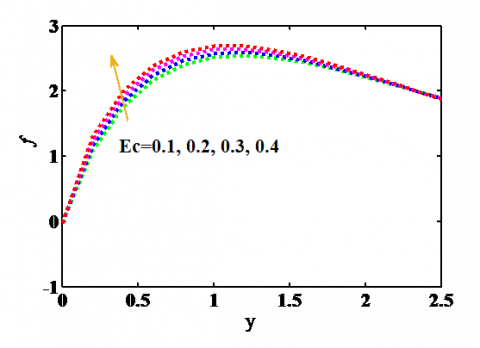
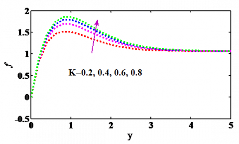
In this study it was selected as t=1.0, n=0.5, ϵ=0.2, & A=0.5 at the same time as Kr, Pr, Gr, Gm, ɳ, k, M, Ra, \gamma and R [28] are varied over a range, which listed in the Figure 2 exhibits the influence of chemical reaction parameter Kr on velocity. Here the incremental values of Kr lead to rise in velocity. Causes the chemical reaction improves momentum transfer moreover consequently accelerates the flow. Figure 3 demonstrates that the effect of distractive Eckert number Ec on the velocity. It seems that, the incremental values of Eckert number Ec leads to enhance in velocity. Due to the Eckert number Ec is the relation between flow kinetic energy to heat enthalpy difference. So, the enhancement of dissimilar values of Eckert number causes rise in the kinetic energy. Figure 4 shows the consequence of porous medium parameter K on the velocity. In this figure based on the outcomes it was found that the enhancement of K leads to rise in velocity. Causes existence of the porous medium in the flow furnishes confrontation to flow. Consequently, the result resistive force tends to sluggish the motion of the fluid along the surface of the plate.
Figure 2. Effect of Kr on Velocity f(y)
Figure 3. Effect of Ec on Velocity f(y)
Figure 4. Effect of K on Velocity f(y)
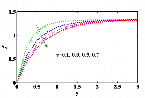
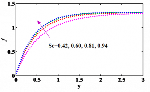
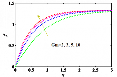
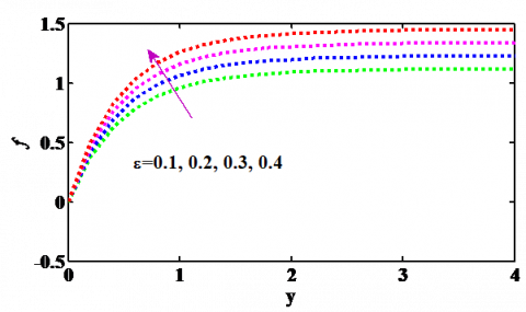
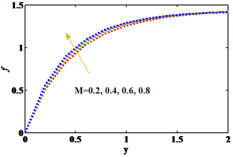
Figure 5 illustrates the effect of Casson fluid model parameter \gamma on the fluid velocity. Form this figure it was found that the fluid velocity reduced with an increase in Casson fluid parameter. This is owing to the enhancement of Casson parameter \gamma , the yield stress falls and hence the momentum boundary layer thickness reduces. Physically, it is observed that raise in \gamma leads to enhance in plastic dynamic viscosity that generate resistance in the flow of fluid and reduce in fluid velocity. Figure 6 exhibits the influence of radiation absorption Ra on the fluid Velocity profile. It is seeming that the fluid velocity rises with the rise in Ra. For dissimilar values of the Schmidt number Sc, the velocity profiles are plotted in Figure 7. It is obvious that the effect of incremental values of Schmidt number results in a rising velocity distribution across the boundary layer. For dissimilar values of solute Grashof number explained on the velocity shown in Figure 8. From this figure it reflects that for disparate enhancement values of Gm leads to ascend in velocity owing to the velocity distribution perpetrate an extreme value in the region and then reduced to move in the direction of a free stream value. For dissimilar values of the Scalar constant \mathcal{E} , the velocity profiles are plotted in Figure 9 from this figure it is obvious that the effect of increasing values of G m results in a rising velocity distribution. The influence of disparate estimators of magnetic field on the velocity illustrated in Figure 10. It can be distinguished that the velocity ascended by means of the rise in magnetic field parameter M. owing to the transverse retrenchment of momentum boundary layer is owing to the applied magnetic field which consequences in the Lorentz force generating substantial resistance to the motion.
Figure 5. Effect of γ on Velocity f(y)
Figure 6. Effect of Ra on Velocity f(y)
Figure 7. Effect of Sc on Velocity f(y)
Figure 8. Effect of Gm on Velocity f(y)
Figure 9. Effect of \varepsilon on velocity f(y)
Figure 10. Effect of M on velocity f (y)
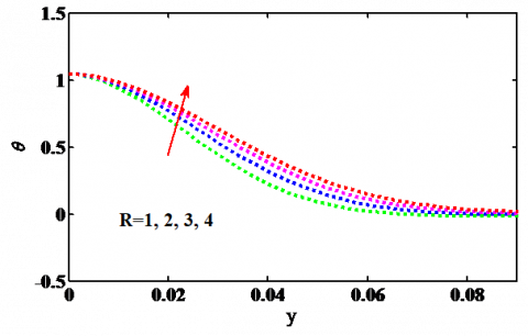
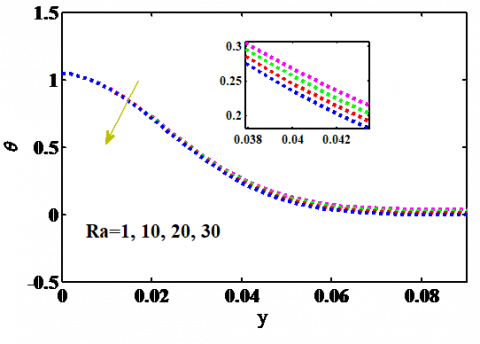
Figure 11 established that for dissimilar values of Prandtl number raises then it leads to reduce in temperature. This is owing to the reality that a higher Prandtl number fluid contains comparatively low thermal conductivity, which diminishes the conduction as an outcome of temperature reduces. As a result, higher Prandtl number show the way to more rapidly cooling of the plate. The influence of disparate estimators of radiation parameter on the temperature is shown Figure 12. From this figure it was disclose that the enhancement of radiation parameter leads to amplify in fluid temperature, with an increasing in the flow boundary layer thickness. Thus, radiation enhances convective flow. Figure 13 exhibits the influence of radiation absorption Ra on the fluid temperature. It seems that for different incremental values of radiation absorption leads to reduce in temperature. For incongruent estimators of the Schmidt number on the fluid concentration is exposed in the Figure 14. From this figure the outcomes indicate that the enhancement of Sc leads to diminished in concentration. This causes the depletion in the concentration is accompanied by instantaneous depletion in the concentration boundary layers, which is perceptible from the Figure 14.
Figure 11. Effect of Pr on temperature θ(y)
Figure 12. Effect of R on Temperature θ(y)
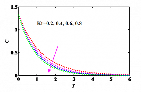
Figure 15 demonstrates the performance of concentration for disparate estimators of chemical reaction (Kr). The results obtain from this figure it was perceived that the concentration reduced due to rise in chemical reaction parameter. For that reason the chemical reaction reinforce momentum transfer and consequently accelerates the flow. The influences of numerical dissimilar parameters are shown on the skin-friction, Nusselt number and Sherwood number. Table 1 represents that the effect of the Gm, Gr, Pr, Sc, Ec, Ra, Kr, K, R, γ, Gr, & ɳ on the skin friction and Nusselt number and Sherwood number respectively. Here the enhancement of different estimators of Sc, R leads to rise in skin friction and nusselt number, However the incremental dissimilar values of Ec, Ra and Pr then it leads to rise Skin friction, but inverse effect was occurred in the case of Nusselt number. In addition, skin friction diminished when the incremental different values of Kr, γ and ɳ, but inverse effect was shown in case of Nusselt number increases. However, for diverse values of Gr and Gm are raises then it led to rise in skin friction. Meanwhile inverse effect was shown in the case of porous medium. And also for dissimilar enhancement values of Sc as well as Kr leads to reduce in Sherwood.
Figure 13. Effect of Ra on temperature θ(y)
Figure 14. Effect of Sc on concentration C(y)
Figure 15. Effect of Kr on concentration C(y)
Table 1. Effect of various parameters on Skin friction, Nussle number and Sherwood number
|
Pr |
Sc |
n |
Ec |
Ra |
Kr |
R |
γ |
Gr |
Gm |
K |
M |
τw |
Nw |
Sh |
|
7 |
0.61 |
0.1 |
0.03 |
0.1 |
2 |
0.1 |
0.5 |
2 |
2 |
1.5 |
2 |
4.1585 |
-23.5246 |
- |
|
10 |
0.60 |
0.1 |
0.03 |
0.1 |
2 |
0.1 |
0.5 |
2 |
2 |
1.5 |
2 |
4.1885 |
-26.5073 |
- |
|
5 |
0.61 |
0.1 |
0.03 |
1 |
2 |
0.01 |
0.5 |
2 |
2 |
1.5 |
0.2 |
3.9866 |
-20.4832 |
-0.8065 |
|
5 |
0.81 |
0.1 |
0.03 |
1 |
2 |
0.01 |
0.5 |
2 |
2 |
1.5 |
0.2 |
4.1935 |
-20.3841 |
-1.0819 |
|
5 |
0.61 |
0.1 |
0.03 |
1 |
2 |
0.01 |
0.5 |
2 |
2 |
1.5 |
0.2 |
3.9909 |
-20.4832 |
- |
|
5 |
0.61 |
0.2 |
0.03 |
1 |
2 |
0.01 |
0.5 |
2 |
2 |
1.5 |
0.2 |
3.9876 |
-19.0220 |
- |
|
5 |
0.61 |
0.1 |
0.01 |
1 |
2 |
0.01 |
0.5 |
2 |
2 |
1.5 |
0.2 |
3.5018 |
-27.0372 |
- |
|
5 |
0.61 |
0.1 |
0.02 |
1 |
2 |
0.01 |
0.5 |
2 |
2 |
1.5 |
0.2 |
3.5052 |
-27.7831 |
- |
|
5 |
0.61 |
0.1 |
0.03 |
5 |
2 |
0.01 |
0.5 |
2 |
2 |
1.5 |
0.2 |
4.0200 |
-21.7107 |
- |
|
5 |
0.61 |
0.1 |
0.03 |
10 |
2 |
0.01 |
0.5 |
2 |
2 |
1.5 |
0.2 |
4.0564 |
-23.2450 |
- |
|
5 |
0.61 |
0.1 |
0.03 |
1 |
0.5 |
0.01 |
0.5 |
2 |
2 |
1.5 |
0.2 |
4.1070 |
-20.9768 |
-1.2321 |
|
5 |
0.61 |
0.1 |
0.03 |
1 |
0.7 |
0.01 |
0.5 |
2 |
2 |
1.5 |
0.2 |
3.9818 |
-20.7928 |
-1.4666 |
|
5 |
0.61 |
0.1 |
0.03 |
1 |
2 |
0.01 |
0.5 |
2 |
2 |
1.5 |
0.2 |
4.1291 |
-20.4832 |
- |
|
5 |
0.61 |
0.1 |
0.03 |
1 |
2 |
0.02 |
0.5 |
2 |
2 |
1.5 |
0.2 |
4.2930 |
-17.6124 |
- |
|
5 |
0.61 |
0.1 |
0.03 |
1 |
2 |
0.01 |
0.1 |
2 |
2 |
1.5 |
0.2 |
5.6560 |
-26.3582 |
- |
|
5 |
0.61 |
0.1 |
0.03 |
1 |
2 |
0.01 |
0.3 |
2 |
2 |
1.5 |
0.2 |
4.1291 |
-26.3221 |
- |
|
5 |
0.61 |
0.1 |
0.03 |
1 |
2 |
0.01 |
0.5 |
5 |
2 |
1.5 |
0.2 |
3.5390 |
- |
- |
|
5 |
0.61 |
0.1 |
0.03 |
1 |
2 |
0.01 |
0.5 |
10 |
2 |
1.5 |
0.2 |
3.6009 |
- |
- |
|
5 |
0.61 |
0.1 |
0.03 |
1 |
2 |
0.01 |
0.5 |
2 |
3 |
1.5 |
0.2 |
3.2533 |
- |
- |
|
5 |
0.61 |
0.1 |
0.03 |
1 |
2 |
0.01 |
0.5 |
2 |
5 |
1.5 |
0.2 |
2.7481 |
- |
- |
|
5 |
0.61 |
0.1 |
0.03 |
1 |
2 |
0.01 |
0.5 |
2 |
2 |
0.4 |
0.2 |
3.1135 |
- |
- |
|
5 |
0.61 |
0.1 |
0.03 |
1 |
2 |
0.01 |
0.5 |
2 |
2 |
1.5 |
0.2 |
3.4984 |
- |
- |
|
5 |
0.61 |
0.1 |
0.03 |
1 |
2 |
0.01 |
0.5 |
2 |
2 |
1.5 |
0.5 |
3.5925 |
- |
- |
|
5 |
0.61 |
0.1 |
0.03 |
1 |
2 |
0.01 |
0.5 |
2 |
2 |
1.5 |
1 |
3.6358 |
- |
- |
This paper is an extended of the work of Rajakumar et al. [28] with Casson fluid parameter γ in the obscene of Casson fluid parameter γ i.e., (\gamma \rightarrow \infty) our results are in good agreement with the results of Rajakumar et al. [28] it was shown from the Table 2.
Table 2. Effect of various physical parameters on Skin friction and Nusselt number
|
Previous study Rajakumar et al. [28] |
Present study if As \gamma \rightarrow \infty |
Present study with Casson fluid parameter \gamma |
|||||
|
|
|
\boldsymbol{\tau}_{\boldsymbol{W}} |
Nw |
\boldsymbol{\tau}_{\boldsymbol{W}} |
Nw |
\boldsymbol{\tau}_{\boldsymbol{W}} |
Nw |
|
Ec |
0.001 |
4.7471 |
-7.5784 |
4.747102 |
-7.578411 |
3.501810 |
-27.037200 |
|
0.003 |
4.7470 |
-7.5784 |
4.747004 |
-7.578421 |
3.505200 |
-27.783100 |
|
|
Ra |
5 |
4.6830 |
-7.7438 |
4.683001 |
-7.743811 |
4.020010 |
-21.710724 |
|
10 |
4.6031 |
-7.9505 |
4.603111 |
-7.950521 |
4.056411 |
-23.245044 |
|
|
ղ |
0.1 |
4.7470 |
-7.5784 |
4.747001 |
-7.578454 |
3.990906 |
-20.483200 |
|
0.2 |
4.7335 |
-6.7563 |
4.733510 |
-6.756310 |
3.987662 |
-19.022000 |
|
|
R |
0.01 |
4.7470 |
-7.5784 |
4.747000 |
-7.578423 |
4.129101 |
-20.483221 |
|
0.02 |
4.7776 |
-5.8289 |
4.7776011 |
-5.828901 |
4.293032 |
-17.612400 |
|
|
Gr |
2 |
4.7470 |
- |
4.747000 |
- |
3.501811 |
- |
|
5 |
4.9103 |
- |
4.9103102 |
- |
3.539010 |
- |
|
The authors are cordially thankful to the honorable reviewers for their constructive comments to improve the quality of the paper. There is no conflict of interest in between the co-authors and there is no funding from any funding agencies.
|
A |
Real positive constant |
|
B0 |
Magnetic induction (A.m-1) |
|
C |
Non dimensional Concentration |
|
Cp |
Specific heat for constant pressure (J.kg −1.K) |
|
C_{w}^{*} |
Concentration of the plate (kg m-3) |
|
Cf |
The local skin-friction (N.m-1) |
|
C_{\infty}^{*} |
Concentration in the fluid far away from the plate( k g \cdot m^{-3} ) |
|
D |
Chemical molecular diffusivity (m2.S-1) |
|
e |
electron charge(C) |
|
E |
Electric field intensity(vm-1) |
|
Ec |
Eckert number |
|
g* |
acceleration due to gravity (m.S-2) |
|
Gm |
Solutal Grashof number |
|
Gr |
local temperature Grashof number |
|
J |
Current density (Am-2) |
|
K |
Permeability of porous medium |
|
Kr |
Chemical reaction parameter (m.S-1) |
|
k_{e}^{*} |
Mean absorption coefficient |
|
k |
Thermal conductivity (W.m-1 .K-1) |
|
M |
Magnetic parameter |
|
N |
Dimensionless material parameter |
|
Nu |
Nusselt number |
|
n |
Mining |
|
py |
yield stress of fluid |
|
Pr |
Prandtl number |
|
Q0 |
Heat generation/absorption |
|
q_{r}^{*} |
Radiation heat flux density (W.m-2) |
|
Ra |
Thermal radiation parameter |
|
R* |
Radiation parameter |
|
Sh |
Sherwood number |
|
Sc |
Schmidt number |
|
T∞ |
Dimensional free stream temperature (K) |
|
T* |
Dimensional Temperature (K) |
|
t* |
dimensional time (S) |
|
T |
Temperature of the fluid (K) |
|
Tw |
Fluid temperature at walls (K) |
|
T_{w}^{*} |
Fluid temperature at the wall (K) |
|
u_{p}^{*} |
Direction of fluid flow |
|
U0 |
Reference velocity at the plate (m S-1) |
|
U_{\infty}^{*} |
Free stream velocity (K) |
|
u |
components of velocity vector in x direction (m.S-1) |
|
v |
Velocity component in y direction (m.S-1) |
|
\mathcal{V}^{*} |
scale of suction velocity |
|
V0 |
Direction of fluid flow |
|
U0 |
components of velocity vector in x direction (m.S-1) |
|
U_{\infty}^{*} |
Scale of suction velocity (m.S-1) |
|
u |
Co-ordinate axis normal to the plate(m) |
|
v |
Scale of suction velocity (m.S-1) |
|
Greek symbols |
|
|
\alpha^{*} |
shear rate |
|
\omega_{e} |
Cyclotron frequency (Hz) |
|
β |
Spin gradient viscosity (K-1) |
|
β* |
Coefficient of volumetric expansion (m3.kg-1) |
|
γ |
Casson fluid parameter |
|
μ |
Fluid dynamic viscosity |
|
ρ |
Density of the fluid (kg.m-3) |
|
υ |
Fluid kinematic viscosity (m2.S‑1) |
|
θ |
Non dimensional temperature (K) |
|
ϵ |
Scalar constant (<<1) |
|
σ |
Electrical conductivity ( \Omega^{-1} m^{-1} ) |
|
\sigma_{s}^{*} |
Stefan-Boltzmann constant (Wm-2K-4) |
|
τw |
Skin-friction coefficient(m2/s) |
|
ɳ |
Heat generation parameter |
|
\tau_{0} |
Casson yield stress |
|
\mu_{B} |
plastic dynamic viscosity |
|
\tau_{e} |
Electron collision time(S) |
\begin{aligned} X_{1} &=\frac{1}{2}\left[-S_{c}+\sqrt{\left(S_{c}\right)^{2}+4 S_{c} K_{r}}\right] \\ & X_{2}=\frac{1}{2}\left[S_{c}+\sqrt{\left(S_{c}\right)^{2}+4 S_{c}\left(K_{r}+n\right)}\right] \\ X_{3} &=\frac{1}{2}\left[3 P_{r}+\sqrt{\left(3 P_{r}\right)-12(3+4 R) \eta P_{r}}\right] \end{aligned}
\begin{aligned} &X_{5}=\frac{1}{2}\left[3 P_{r}+\sqrt{\left(3 P_{r}\right)^{2}+12 P_{r}(3+4 R)(n-\eta)}\right]\\ &X_{4}=\frac{1}{2}[1+\sqrt{1+4 \phi}], X_{6}=\frac{1}{2}[1+\sqrt{1+4(\phi+n)}] \end{aligned}
{{h}_{1}}=\frac{{{R}_{1}}{{S}_{c}}A}{X_{1}^{2}-{{X}_{1}}{{S}_{c}}-{{S}_{c}}\left( {{K}_{r}}+n \right)}
{{h}_{2}}=\frac{-3{{P}_{r}}{{R}_{a}}}{\left( 3+4R \right)X_{1}^{2}-3{{P}_{r}}{{X}_{1}}+3{{P}_{r}}n}
h_{3}=\frac{G_{r}\left(1-N_{2}\right)}{X_{3}^{2}-X_{3}-\phi} h_{4}=\frac{-\left(G_{r} h_{2}+G_{m}\right)}{X_{1}^{2}-X_{1}-\phi}
{{h}_{6}}=\frac{-3{{P}_{r}}h_{3}^{2}X_{3}^{2}}{4X_{3}^{2}\left( 3+4R \right)-6{{P}_{r}}{{X}_{3}}+3\eta {{P}_{r}}}
{{h}_{7}}=\frac{-3{{P}_{r}}h_{4}^{2}X_{1}^{2}}{4X_{1}^{2}\left( 3+4R \right)-6{{P}_{r}}{{X}_{1}}+3\eta {{P}_{r}}}
{{h}_{7}}=\frac{-3{{P}_{r}}h_{4}^{2}X_{1}^{2}}{4X_{1}^{2}\left( 3+4R \right)-6{{P}_{r}}{{X}_{1}}+3\eta {{P}_{r}}}
{{h}_{9}}=\frac{-6{{P}_{r}}{{N}_{3}}{{X}_{3}}{{h}_{4}}{{X}_{1}}}{{{\left( {{X}_{1}}+{{X}_{3}} \right)}^{2}}\left( 3+4R \right)-3{{P}_{r}}\left( {{X}_{1}}+{{X}_{3}} \right)+3\eta {{P}_{r}}}
{{h}_{10}}=\frac{-6{{P}_{r}}{{X}_{4}}{{A}_{0}}{{h}_{4}}{{X}_{1}}}{\left( 3+4R \right){{\left( {{X}_{1}}+{{X}_{4}} \right)}^{2}}-3{{P}_{r}}\left( {{X}_{1}}+{{X}_{4}} \right)+3\eta {{P}_{r}}}
\begin{aligned} &h_{11}=\frac{-G_{r} A_{1}}{X_{3}^{2}-X_{3}-\phi} h_{12}=\frac{-G_{r} h_{5}}{4 X_{4}^{2}-2 X_{4}-\phi}\\ &h_{13}=\frac{-G_{r} h_{6}}{4 X_{3}^{2}-2 X_{3}-\phi} h_{14}=\frac{-G_{r} h_{7}}{4 X_{1}^{2}-2 X_{1}-\phi} \end{aligned}
\begin{aligned} &h_{15}=\frac{-G_{r} h_{8}}{\left(X_{3}+X_{4}\right)^{2}-\left(X_{3}+X_{4}\right)-\phi}\\ &\begin{array}{l} h_{16}=\frac{-G_{r} h_{9}}{\left(X_{1}+X_{3}\right)^{2}-\left(X_{1}+X_{3}\right)-\phi} \\ h_{17}=\frac{-G_{r} h_{10}}{\left(X_{1}+X_{4}\right)^{2}-\left(X_{1}+X_{4}\right)-\phi} \\ h_{18}=\frac{3 A P_{r} X_{1} h_{2}-3 P_{r} X_{9} h_{1}}{X_{1}^{2}(3+4 R)-3 P_{r} X_{1}-3 P_{r}(n-\eta)} \end{array} \end{aligned}
\begin{aligned} &h_{19}=\frac{-3 P_{r} R_{a}\left(1-h_{1}\right)}{X_{2}^{2}(3+4 R)-3 P_{r} X_{2}-3 P_{r}(n-\eta)}\\ &h_{20}=\frac{-3 A P_{r} X_{13}\left(1-h_{2}\right)}{X_{3}^{2}(3+4 R)-3 P_{r} X_{3}-3 P_{r}(n-\eta)}\\ &h_{21}=\frac{A h_{4} X_{1}-G_{r} h_{18}-G_{m} h_{1}}{X_{1}^{2}-X_{1}-(n+\phi)} \quad h_{22}=\frac{-G_{r} h_{19}-G_{m}\left(1-h_{1}\right)}{X_{2}^{2}-X_{2}-(n+\phi)}\\ &h_{23}=\frac{A h_{3} X_{3}-G_{r} h_{20}}{X_{3}^{2}-X_{3}-(\phi+n)} \quad h_{24}=\frac{A A_{0} X_{4}}{X_{4}^{2}-X_{4}-(n+\phi)}\\ &h_{25}=\frac{-A_{3} G_{r}}{X_{5}^{2}-X_{5}-(n+\phi)} \end{aligned}
\begin{aligned} &h_{26}=\frac{-6 P_{r} A_{0} X_{4} X_{2} h_{22}}{(3+4 R)\left(X_{2}+X_{4}\right)^{2}-3 P_{r}\left(X_{2}+X_{4}\right)-3 P_{r}(n-\eta)}\\ &h_{27}=\frac{-6 P_{r} A_{0} X_{4} h_{2} X_{3}+3 A P_{r}\left(X_{3}+X_{4}\right)-6 P_{r} h_{3} X_{3} h_{24} X_{4}}{(3+4 R)\left(X_{4}+X_{3}\right)^{2}-3 P_{r}\left(X_{4}+X_{3}\right)-3 P_{r}(n-\eta)}\\ &h_{28}=\frac{-6 P_{r} A_{0} X^{2} h_{24}+6 A P_{r} X_{4} h_{5}}{4 X_{4}^{2}(3+4 R)-6 P_{r} X_{4}-3 P_{r}(n-\eta)}\\ &h_{29}=\frac{-6 P_{r} A_{0} X_{4} X_{6} A_{4}}{(3+4 R)\left(X_{4}-X_{6}\right)^{2}-3 P_{r}\left(X_{4}+X_{6}\right)-3 P_{r}(n-\eta)} \end{aligned}
\begin{aligned} &h_{30}=\frac{-6 P_{r} A_{0} X_{4} h_{25} X_{5}}{\left(X_{4}-X_{5}\right)^{2}(3+4 R)-3 P_{r}\left(X_{4}+X_{5}\right)-3 P_{r}(n-\eta)}\\ &\begin{array}{l} h_{31}=\frac{-6 P_{r} h_{3} X_{3} X_{1} h_{21}+3 A P_{r}\left(X_{1}+X_{3}\right) h_{9} h_{3}-6 P_{r} h_{4} X_{1} h_{23} X_{3}}{\left(X_{1}+X_{3}\right)^{2}(4+3 R)-3 P_{r}\left(X_{1}+X_{3}\right)-3 P_{r}(n-\eta)} \\ h_{32}=\frac{-6 P_{r} h_{3} X_{3} X_{2} h_{22}}{(4+3 R)\left(X_{3}+X_{2}\right)^{2}-3 P_{r}\left(X_{3}+X_{2}\right)-3 P_{r}(n-\eta)} \\ h_{32}=\frac{-6 P_{r} h_{3} X_{3} X_{2} h_{22}}{(4+3 R)\left(X_{3}+X_{2}\right)^{2}-3 P_{r}\left(X_{3}+X_{2}\right)-3 P_{r}(n-\eta)} \end{array}\\ &h_{33}=\frac{-6 P_{r} h_{3} X_{3}^{2} h_{23}+6 P_{r} A X_{3} h_{6}}{4 X_{3}^{2}-6 X_{3} P_{r}-3 P_{r}(n-\eta)} \end{aligned}
\begin{array}{l} h_{34}=\frac{-6 P_{r} h_{3} X_{3} X_{6} A_{4}}{(4+3 R)\left(X_{3}+X_{6}\right)^{2}-3 P_{r}\left(X_{3}+X_{6}\right)-3 P_{r}(n-\eta)} \\ h_{55}=\frac{-6 P h_{3} X_{3} h_{5} X_{5}}{(4+3 R)\left(X_{3}+X_{5}\right)^{2}-3 P_{r}\left(X_{3}+X_{5}\right)-3 P_{r}(n-\eta)} \\ h_{36}=\frac{-6 P h_{4} X_{1}^{2} h_{21}+6 A P_{r} X_{1} h_{7}}{4 X_{1}^{2}(4+3 R)-6 P_{r} X_{1}-3 P_{r}(n-\eta)} \\ h_{37}=\frac{-6 P h_{4} X_{1} X_{2} h_{2}}{(4+3 R)\left(X_{1}+X_{2}\right)^{2}-3 P_{r}\left(X_{1}+X_{2}\right)-3 P_{r}(n-\eta)} \end{array}
[1] Patel, H.R. (2019) Effects of cross diffusion and heat generation on mixed convective MHD flow of Casson fluid through porous medium with non-linear thermal radiation. Heliyon, 5(4): 1-26. https://doi.org/10.1016/j.heliyon.2019.e01555
[2] Kataria, H.R., Patel, H.R. (2019) Effects of chemical reaction and heat generation/absorption on MHD Casson fluid flow over an exponentially accelerated vertical plate embedded in porous medium with ramped wall temperature and ramped surface concentration. Propulsion and Power Research, 8(1): 35-46. https://doi.org/10.1016/j.jppr.2018.12.001
[3] Biswas, R., Mondal, M., Sarkar, D.R., Ahmmed, S.F. (2017). Effects of radiation and chemical reaction on MHD unsteady heat and mass transfer of Casson fluid flow past a vertical plate. Journal of Advances in Mathematics and Computer Science, 23(2): 1-16. https://doi.org/10.9734/JAMCS/2017/34292
[4] Srinivasa Raju, Jithender Reddy, R., Anitha, G. (2017). MHD Casson viscous dissipative fluid flow past a vertically inclined plate in presence of heat and mass transfer. Frontiers in Heat and Mass Transfer, 8(27): 1-15. https://doi.org/10.5098/hmt.8.27
[5] Khalid, A., Khan, I., Khan, A., Shafie, S. (2015) Unsteady MHD free convection flow of Casson fluid past over an oscillating vertical plate embedded in a porous medium. Engineering Science and Technology, an International Journal, 8(3): 309-317. https://doi.org/10.1016/j.jestch.2014.12.006
[6] Jithender Reddy, G., Srinivasa Raju, R., Anand Rao, J. (2017). Influence of viscous dissipation on unsteady MHD natural convective flow of Casson fluid over an oscillating vertical plate. Ain Shams Engineering Journal, 9(4): 1907-1915. https://doi.org/10.1016/j.asej.2016.10.012
[7] Kataria, H.R., Patel, H.R. (2016). Radiation and chemical reaction effects on MHD Casson fluid flow past an oscillating vertical plate embedded in porous medium. Alexandria Engineering Journal, 55(1): 583-595. https://doi.org/10.1016/j.aej.2016.01.019
[8] Ramamohan Reddy, L., Raju, M.C., Raju, G.S.S., Reddy, N.A. (2016) Thermal diffusion and rotational effects on magneto hydrodynamic mixed convection flow of heat absorbing/generating visco-elastic fluid through a porous channel, front. Heat Mass Transfer, 7(20): 1-15. https://doi.org/10.5098/hmt.7.20
[9] El-Aziz, M.A., Afify, A.A. (2016). Effects of variable thermal conductivity with thermal radiation on MHD flow and heat transfer of Casson liquid film over an unsteady stretching surface. Brazilian Journal of Physics, 46(5): 516-525. https://doi.org/10.1007/s13538-016-0442-3
[10] Srinivasa Raju, R., Jithender Reddy, G., Anitha, G. (2017). MHD Casson viscous dissipative fluid flow past a vertically inclined plate in presence of heat and mass transfer-Finite element technique. Frontiers in Heat and Mass Transfer, 8(27): 1-12. http://dx.doi.org/10.5098/hmt.8.27
[11] Srinivasa Raju, R., Mahesh Reddy, B., Jithender Reddy, G. (2017). Finite element solutions of free convective Casson fluid flow past a vertically inclined plate submitted in magnetic field in presence of heat and mass transfer. Int., J., for Comput. Methods in Eng. Scie. & Mechanics, 18(4-5): 250-265. https://doi.org/10.1080/15502287.2017.1339139
[12] Saidulu, N., Venkata Lakshm, A. (2016). MHD flow of Casson fluid with slip effects over an exponentially porous stretching sheet in presence of thermal radiation, viscous dissipation and heat source/sink. American Research Journal of Mathematics, 2: 1-15. https://doi.org/10.21694/2378-704X.16001
[13] Pushpalatha, K., Sugunamma, V., Ramana Reddy, J.V., Sandeep, N. (2016). Heat and mass transfer in unsteady MHD Casson fluid flow with convective boundary conditions. International Journal of Advanced Science and Technology, 91: 19-38. https://doi.org/10.14257/ijast.2016.91.03
[14] Vajravelu, K., Hdjinicolaou, A. (1993) Heat transfer in a viscous fluid over a stretching sheet with viscous dissipation and internal heat generation. International Communication in Heat and Mass Transfer, 20(3): 417-430. https://doi.org/10.1016/0735-1933(93)90026-R
[15] Suresh, B., Veena, P.H., Pravin, V.K. (2016). Free convective heat transfer flow of a Casson fluid with radiative and dissipative effect due to variable thermal conductivity and internal heat generation past a stretching sheet. International Journal of Engineering Sciences & Research Technology, 5(10): 638-654. https://doi.org/10.5281/zenodo.163079
[16] Venkateswarlu, B., Satya Narayana, P.V. (2016). Influence of variable thermal conductivity on MHD Casson fluid flow over a stretching sheet with viscous dissipation, soret and dufour effects. Front in Heat Mass Transfer, 7(16): 25-35. https://doi.org/10.5098/hmt.7.16
[17] Qasim M., Ahmad, B. (2015). Numerical solution for the blasius flow in a Casson fluid with viscous dissipation and convective boundary conditions. Heat Transfer Research, 46(8): 689-697. https://doi.org/10.1615/HeatTransRes.2015007148
[18] Venkateswarlu, S., Varma, S.V.K., Kiran Kumar, R.V.M.S.S., Raju, C.S.K., Durga Prasad, P. (2017). Radiation absorption and viscous-dissipation on MHD flow of Casson fluid over a vertical plate filled with porous layers. Diffusion Foundations, 11: 43-56. https://doi.org/10.4028/www.scientific.net/DF.11.43
[19] Harinath Reddy, S., Raju, M.C., Keshava Reddy, E. (2016). Radiation absorption and chemical reaction effects on MHD flow of heat generating Casson fluid past oscillating vertical porous plate. Front in Heat Mass Transfer, 7(21): 21-30. https://doi.org/10.5098/hmt.7.21
[20] Reddy, B.A.P. (2016). MHD flow of a Casson fluid over an exponentially inclined permeable stretching surface with thermal radiation and chemical reaction. Ain Shams Engineering Journal, 7(2): 593-602. https://doi.org/10.1016/j.asej.2015.12.010
[21] Ullah, I., Bhattacharyya, K., Shafie, S., Khan, I. (2016). Unsteady MHD mixed convection slip flow of Casson fluid over nonlinearly stretching sheet embedded in a porous medium with chemical reaction, thermal radiation, heat absorption and convective boundary conditions. PLoS ONE. 11(10): e0165348. https://doi.org/10.1371/journal.pone.0165348
[22] Eswara Rao, M., Sreenadh, S. (2017). MHD flow of a Casson fluid over an exponentially inclined permeable stretching surface with thermal radiation, viscous dissipation and chemical reaction. Global Journal of Pure and Applied Mathematics, 13(10): 7529-7548.
[23] Durairaj, M., Ramachandran, S., Mehdi, R.M. (2017). Heat generating/absorbing and chemically reacting Casson fluid flow over a vertical cone and flat plate saturated with non-Darcy porous medium. International Journal of Numerical Methods for Heat and Fluid Flow, 27(2): 156-173. https://doi.org/10.1108/HFF-08-2015-0318
[24] Jasmine Benazir, A., Sivaraj, R., Makinde, O.D. (2016). Unsteady MHD Casson fluid flow over a vertical cone and flat plate with non-uniform heat source/sink. International Journal of Engineering Research in Africa, 21(1): 69-83. https://doi.org/10.4028/www.scientific.net/JERA.21.69
[25] Rajakumar, K.V.B., Balamurugan, K.S., Ramana Murthy, C.V., Umasenkara Reddy, M. (2017). Chemical reaction and viscous dissipation effects on MHD free convective flow past a semi-infinite moving vertical porous plate with radiation absorption. Global Journal of Pure and Applied Mathematics, 13(12): 8297-8322.
[26] Ramaiah. Vijaya Kumar Varma., Rama Krishna Prasad & Balamurugan. (2016) Chemical reaction and radiation absorption effects on MHD convective heat and mass transfer flow of a viscoelastic fluid past an oscillating porous plate with heat generation/absorption. Int. J. Chem. Sci., 14(2): 570-584.
[27] Rajakumar, K.V.B., Balamurugan, K.S., Ramana Murthy, C.V. (2018). Radiation absorption and viscous dissipation effects on MHD free convective flow past a semi-infinite moving vertical porous plate. International Journal of Fluid Mechanics Research, 45(5): 439-458. https://doi.org/10.1615/InterJFluidMechRes.2018024790
[28] Rajakumar, K.V.B., Ramana Murthy, C.V., Balamurugan, K.S. (2018). Radiation, dissipation and Dufour effects on MHD free convection Casson fluid flow through a vertical oscillatory porous plate with Ion-slip current. International Journal of Heat and Technology, 36(2): 494-508. https://doi.org/10.18280/ijht.360214