Nagaraju Gajjela* | Mahesh Garvandha | Anjanna Matta
OPEN ACCESS
This paper examines the impact of reactive diffusion(mass) transport with the application of magnetic field vertical to the flow direction where the Newtonian fluid is passing over a circular pipe. Uniform suction is applied, externally, across the wall in the transverse direction. A strong analytical methodology, specifically, the homotopy analysis method (HAM) is employed to realize solutions to the non-linear coupled equations. The effect of magnetic parameter $(M),$ suction Reynold number $(R e),$ Schmidt parameter $(S c),$ first-order chemical reaction parameter( $\gamma)$ on velocity components and concentration are displayed graphically and explained numerically. The dimensionless of axial concentration $\phi$ decrease for a given rise in $\gamma .$ Further, the behavior is inverted i.e. for the cases of radial concentration $\phi$ increases as $\gamma$ increases.
mass transfer, suction, magnetic field, chemical reaction, Newtonian fluid, HAM
In recent years, engineers have additionally investigated the modification of Newtonian flows via wall porousness of the channel or pipe. The wall Injection/removal of fluid via pores may be a strong mechanism for flow management. This technology quality vital potential in bio-medical engineering (e.g. artificial qualitative analysis, blood circulation) and in different engineering areas like rocket technology & food process.
Consequently, mathematical modeling of this type of flow through surface mass flux pipes has stimulated some interest in the research community. Intilaly the study laminar flow in 2-D channel was examined by Berman [l], Sellars [2] and Yuana [3]. Later Bansal [4] extended this work through a permeable circular pipe to a steady, viscous flow. He obtained an analytical solution for velocity under the influence of suction/injection parameter and pressure gradient in z-direction. An analytical expression for the Newtonian flow over the pipe underneath uniform wall suction/injection was any reportable by Terril [5, 6]. Tsangaris and Kondaxakis [7] thought of time-dependent Newtonian flow in an exceedingly porous pipe. He obtained an analytical solution for time-varying wall injection/suction concerning the pipe. Cox and Hill [8] examined the Newtonian fluid flow with a Navier slip at the wall through carbon nanotubes. They recognized the maximum flow rate for the standard Poiseuille flow, which happens for steady inward-directed flow across the boundary. Ramana murthy et al. [9] studied micropolar flow developed by a permeable cylinder exhibiting rotary oscillations, they have concluded that the tangential drag decreases with suction parameter will increase. In 2-phase flow between two porous plates, Srinivas and Ramana Murthy [10] studied wall suction effects. They found that Darcy parameter will increase the velocity of the fluid.
Magnetohydrodynamics (MHD) is also an active area of modern engineering sciences and involves the interaction of magnetic fields and conduction of electrical fluids. MHD tube flows arise in ion accelerators, MHD flow management in nuclear reactors, liquid metal fabrication processes, bubble levitation, etc. MHD flows that includes suction/injection wall effects have garnered considerable attention. Terrill and Shrestha [11] found that, with an increase in magnetic number, wall friction increases. Attia [12] investigated the unstable laminar flow of 2-phase non-Newtonian liquids through a circular tube between a pressure gradient at z-direction. He concluded that the velocity and temperature components for both phases decrease as Magnetic parameter increases. Attia and Ahmed [13] computed solutions for unsteady magnetic Bingham plastic flow in a circular tube. They found an increase in the viscosity of the particles and skin friction. El-Shahed [14] examined the impact of the transverse magnetic field in a porous material on the transient viscoelastic fluid flow. In terms of Fox's H-function, he found the solution velocity. Ramanamurthy and Bahali [15] investigated the effects of wall suction/injection on magneto-micropolar transport in a porous circular tube. They recognized that shear stress (skin friction) at wall is boosted with a greater magnetic number. Murthy et al. [16] considered the impact on the micropolar flow in a rectangular duct of the magnetic parameter, wall suction / blowing. They found that larger magnetic fields decelarate the magnitudes of the flow rate.
Implication of mass transfer study is very important in the fields of engineering, Industries and sciences. Applications of this study are found in many branches of engineering and industry such as the safety of nuclear reactor, reaction engineering, absorption resistance, chemical and metallurgical industry etc. In day to day life also, we observe in the dissolution of sugar added to a cup of coffee and diffusion of smoke through tall chimneys into the environment. Hayat et al. [17] found the impact of chemical reaction on Maxwell fluid in a porous channel. They notice that the velocity in viscoelastic fluid has an inverse conduct by raising the amount of Reynolds number. Bridges and Rajagopal [18] examined the pulsatile flow of a chemical reactive fluid. They notice that the fluid concentration near the centerline rises with distinct cycles of time. Other interesting and recent investigations into pipe dynamics have been communicated in previous studies [19-28].
Our study aims to examine the impact of suction, chemical reaction and magnetic field on two-dimensional incompressible Newtonian fluid flow in a circular pipe. By using the powerful homotopy analysis method (HAM) [29] we find the solutions for the non-dimensional equations. We have studied the effect of Schmidt number, Suction Reynold number, magnetic number, and chemical reaction on velocity components and concentration and presented the results graphically.
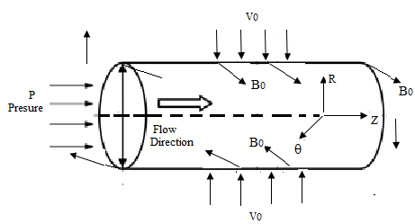
Figure 1 shows an endless circular radius tube in which Newtonian fluid flows. The system of mass transfer is studied throughout uniform mass flux on the axis of the pipe and constant mass at the surface of the pipe, ignoring the effects of thickness of the pipe. As the tube is of semi infinite length, the flow is considered to be fully developed. This flow is exposed to an outwardly applied perpendicular suction across the wall and a constant magnetic force field B0 in polar direction. The number of magnets is small enough to neglect the effects of the magnetic field being induced. The primitive equations for viscous flow [30] are:
Figure 1. Schematic diagram
$\frac{\partial U}{\partial R}+\frac{U}{R}+\frac{\partial W}{\partial Z}=0$ (1)
$\rho\left(U \frac{\partial U}{\partial R}+W \frac{\partial U}{\partial Z}\right)=-\frac{\partial P}{\partial R}+\mu \frac{\partial}{\partial Z}\left(\frac{\partial U}{\partial Z}-\frac{\partial W}{\partial R}\right)-\sigma B_{0}^{2} U$ (2)
$\rho\left(U \frac{\partial W}{\partial R}+W \frac{\partial W}{\partial Z}\right)=-\frac{\partial P}{\partial Z}-\frac{\mu}{R} \frac{\partial}{\partial R}\left(R\left(\frac{\partial U}{\partial Z}-\frac{\partial W}{\partial R}\right)\right)-\sigma B_{0}^{2} W$ (3)
$U \frac{\partial c}{\partial R}+W \frac{\partial c}{\partial z}=D\left(\frac{\partial^{2} c}{\partial R^{2}}+\frac{1}{R} \frac{\partial c}{\partial R}+\frac{\partial^{2} C}{\partial z^{2}}\right)-k_{1} C$ (4)
The boundary conditions on the axis are obtained by taking the flow to be symmetrical, so that
$\text { At } \mathrm{R}=0, \frac{\partial W}{\partial R}=U=\frac{\partial C}{\partial R}=0$ At $\mathrm{R}=a, W=0, U=v_{0},$ and $C=C_{w}$
In the following equations, upper case letters denote physical (dimensional) quantities and the corresponding non-dimensional amounts represent lower case letters:
$U=u v_{0}, W=w v_{0}, R=r a, P=\rho p v_{0}^{2}, Z=z a, \phi=\frac{c-c_{0}}{c_{w}-c_{0}}$ (5)
Implementing Eq. (5) into Eqns. (1)-(4), following the dimensionless system of non-linear coupled equations, emerges:
$\frac{\partial u}{\partial r}+\frac{u}{r}+\frac{\partial w}{\partial z}=0$ (6)
$\operatorname{Re}\left(u \frac{\partial u}{\partial r}+w \frac{\partial u}{\partial z}\right)=-\operatorname{Re} \frac{\partial p}{\partial r}+\frac{\partial}{\partial z}\left(\frac{\partial u}{\partial z}-\frac{\partial w}{\partial r}\right)-M^{2} u$ (7)
$\operatorname{Re}\left(u \frac{\partial w}{\partial r}+w \frac{\partial w}{\partial z}\right)=-\operatorname{Re} \frac{\partial p}{\partial z}-\frac{1}{r} \frac{\partial}{\partial r}\left(r\left(\frac{\partial u}{\partial z}-\frac{\partial w}{\partial r}\right)\right)-M^{2} w$ (8)
$\begin{aligned} \operatorname{Re} S c\left(u \frac{\partial \phi}{\partial r}+w \frac{\partial \phi}{\partial z}\right)=\frac{\partial^{2} \phi}{\partial r^{2}}+\frac{1}{r} \frac{\partial \phi}{\partial r}+\frac{\partial^{2} \phi}{\partial z^{2}}-S c\left(K_{1}+\gamma \phi\right) \end{aligned}$(9)
$\operatorname{Re}=\frac{\rho v_{0} a}{\mu}, M^{2}=\frac{\sigma B_{0}^{2} a^{2}}{\mu}, S c=\frac{v}{D}, \gamma=\frac{k_{1} a^{2}}{v} \quad$ and
$K_{1}=\frac{k_{1} C_{0} a^{2}}{v\left(C_{w}-C_{0}\right)}$
Now, we incorporate a stream function ψ [11] that will satisfy the continuity, Eq. (6)
$\psi=(N-z) f(r)$ (10)
The components of axial and radial velocity can be taken as
$u=-\frac{1}{r} \frac{\partial \psi}{\partial z}, w=\frac{1}{r} \frac{\partial \psi}{\partial r}$ (11)
Replacing Eq. (11) in Eqns. (7) and (8) and then the pressure term is removed, we get
$\operatorname{Re}\left(-\frac{2}{r^{3}} \frac{\partial \psi}{\partial z} E^{2} \psi+\frac{1}{r^{2}}\left(\frac{\partial \psi}{\partial z} \frac{\partial E^{2} \psi}{\partial r}-\frac{\partial \psi}{\partial r} \frac{\partial E^{2} \psi}{\partial z}\right)\right)=\frac{-1}{r} E^{2}\left(E^{2} \psi\right)+\frac{M^{2}}{r} E^{2} \psi$ (12)
where, $E^{2}=\frac{\partial^{2}}{\partial r^{2}}-\frac{1}{r} \frac{\partial}{\partial r}+\frac{\partial^{2}}{\partial z^{2}}$ .
Using Eq. (10) in equation (12) we get,
$\begin{aligned} R e &=\left\{2 f \cdot D^{2} f+r\left(f^{\prime} \cdot D^{2} f-f \cdot \frac{d}{d r} D^{2} f\right)\right\} =r^{2} D^{2}\left(-D^{2}+M^{2}\right) f \end{aligned}$
Or, alternately,
$\operatorname{Re}\left(\frac{3 f f^{\prime \prime}}{r^{2}}-\frac{3 f f^{\prime}}{r^{3}}-\frac{f f^{\prime \prime \prime}}{r}+\frac{f_\prime f^{\prime \prime}}{r}-\frac{f^{\prime 2}}{r^{2}}\right)=D^{2}\left(-D^{2}+M^{2}\right) f$ (13)
where, $D^{2}=\frac{d^{2}}{d r^{2}}-\frac{1}{r} \frac{d}{d r}$ is a differential operator.
The corresponding boundary conditions are
$\left.\begin{array}{l}{f=D^{2} f=\frac{\partial \phi}{\partial r}=0 \text { at } \mathrm{r}=0.} \\ {f_\prime=0, f=\phi=1 \text { at } \mathrm{r}=1}\end{array}\right\}$ (14)
For the HAM approximation of Eqns. (9) and $(13),$ we propose the Eq. ( 15) as the boundary conditions from the Eq. $(14),$ the initial (zero order) approximations for $f_{0}$ and $\phi_{0}$ and auxiliary linear operators $L_{1}$ and $L_{2}$ are as follows:
$\begin{aligned} f(0)=0, & D^{2} f(0)=0, f(1)=1, f^{\prime}(1)=0, \phi^{\prime}(0)=0 \text { and } \phi(1)=1 \end{aligned}$ (15)
$f_{0}=r^{2}\left(2-r^{2}\right)$ and $\phi_{0}(r)=1$
$L_{1}[f]=D^{4} f$ and $L_{2}[\phi]=\nabla^{2} \phi$
With $L_{1}\left[c_{1} r^{4}+c_{2} r^{2}(2 \log r-1)+c_{3} r^{2}+c_{4}\right]=0$
$L_{2}\left[(N-z)^{2}\left(c_{5}+c_{6} \log r\right)+c_{7} r^{2}+c_{8} r^{2}(\log r-1)\right]$=0 (16)
where, $C_{i}$(i = 1–8) are constants.
3.1 Zeroorder deformation equations
The zero order deformation Eqns. for (13) and (9) can be written as follows:
$(1-\lambda) L_{1}\left[f(r, \lambda)-f_{0}(r)\right]=\lambda h_{1} H N_{1}(f(r, \lambda))$ (17)
$f(0, \lambda)=D^{2} f(0, \lambda)=f^{\prime}(1, \lambda)=0, f(1, \lambda)=1$ (18)
$(1-\lambda) L_{2}\left[\phi(r, z, \lambda)-\phi_{0}(r)\right]=\lambda h_{2} H N_{2}(\phi(r, z, \lambda), f(r, \lambda))$ (19)
$\phi(1, \lambda)=1, \quad \phi^{\prime}(0, \lambda)=0$ (20)
where,
$N_{1}[f(r, \lambda)]=D^{2}\left(-D^{2}+M^{2}\right) f(r, \lambda)-\frac{R e}{r^{3}}\left(\begin{array}{c}{3 r f(r, \lambda) \frac{\partial^{2} f(r, \lambda)}{\partial r^{2}}-3 f(r, \lambda) \frac{\partial f(r, \lambda)}{\partial r}-r^{2} f(r, \lambda) \frac{\partial^{3} f(r, \lambda)}{\partial r^{3}}} \\ {+r^{2} \frac{\partial f(r, \lambda)}{\partial r} \frac{\partial^{2} f(r, \lambda)}{\partial r^{2}}-r\left(\frac{\partial f(r, \lambda)}{\partial r}\right)^{2}}\end{array}\right)$ (21)
$\begin{aligned} N_{2}(\phi(r, z, \lambda), f(r, \lambda))=& \operatorname{Re} \operatorname{Sc}\left(\frac{f(r, \lambda)}{r}\left((N-z)^{2} \frac{\partial \phi_{1}(r, \lambda)}{\partial r}+\right.\right.\\\left.\left.\frac{\partial \phi_{2}(r, \lambda)}{\partial r}\right)-2 \frac{(N-z)^{2}}{r} \phi_{1}(r, \lambda) \frac{\partial f(r, \lambda)}{\partial r}\right)-\left((N-z)^{2}\left(\frac{\partial^{2} \phi_{1}(r, \lambda)}{\partial r^{2}}+\right.\right.\\\left.\frac{1}{r} \frac{\partial \phi_{1}(r, \lambda)}{\partial r}\right)+\left(\frac{\partial^{2} \phi_{2}(r, \lambda)}{\partial r^{2}}+\frac{1}{r} \frac{\partial \phi_{2}(r, \lambda)}{\partial r}+2 \phi_{1}(r, \lambda)\right)+\operatorname{Sc} \gamma((N-\\\left.z)^{2} \phi_{1}(r, \lambda)+\phi_{2}(r, \lambda)\right)+S c K_{1} \end{aligned}$ (22)
With $\phi(r, z, \lambda)=(N-z)^{2} \phi_{1}(r, \lambda)+\phi_{2}(r, \lambda)$
Here $\lambda \in[0,1]$ is a homotopy parameter, $h_{1}$ and $h_{2}$ are the convergence control parameters, H is the auxiliary function (taken as 1)
For $\lambda=0$ and $\lambda=1,$ we have $f(r, 0)=f_{0}(r)$
$f(r, 1)=f(r), \phi(r, 0)=\phi_{0}(r), \phi(r, 1)=\phi(r)$ (23)
Further, by Maclaurin’s series expansion, one gets
$f(r, \lambda)=f_{0}(r)+\sum_{n=1}^{\infty} f_{n}(r) \lambda^{n}$ (24)
where, $f_{n}(r)=\frac{1}{n !} \frac{\partial^{n} f(r, \lambda)}{\partial \lambda^{n}}$.
$\phi(r, \lambda)=\phi_{0}(r)+\sum_{n=1}^{\infty} \phi_{n}(r) \lambda^{n}$ (25)
where,$\phi_{n}(r)=\frac{1}{n !} \frac{\partial^{n} \phi(r, \lambda)}{\partial \lambda^{n}}$.
We choose $h_{1}$ and $h_{2},$ suitably just as these succession are convergent at $\lambda=1,$ hence the expressions of solution from Eqns. (24)-(25) as follows:
$f(r)=f_{0}(r)+\sum_{n=1}^{\infty} f_{n}(r)$ (26)
$\phi(r)=\phi_{0}(r)+\sum_{n=1}^{\infty} \phi_{n}(r)$ (27)
3.2 The higher order deformation equation
Differentiating n times for Eqns. (17)-(20) with respect to parameter $\lambda,$ next multiply by $\frac{1}{n !}$ And subsequently we get the equations of nth order as follows:
$L_{1}\left[f_{n}(r)-\Upsilon_{n} f_{n-1}(r)\right]=h_{1} R_{1, n}(r)$ (28)
$L_{2}\left[\phi_{n}(r)-\Upsilon_{n} \phi_{n-1}(r)\right]=h_{2} R_{2, n}(r)$ (29)
where,
$R_{1, n}(r)=D^{2}\left(-D^{2}+M^{2}\right) f_{n-1}-\frac{R e}{r^{3}} \sum_{i=0}^{n-1}\left(3 r f_{i} f_{n-1-i}^{\prime \prime}-\right.\left.3 f_{i} f^{\prime}_{n-1-i}-r^{2} f_{i} f^{\prime \prime \prime}_{n-1-i}+r^{2} f_{i}^{\prime} f_{i}^{\prime \prime} f_{n-1-i}^{\prime \prime}-r f_{i}^{\prime} f_{n-1-i}^{\prime}\right)$ (30)
and
$R_{2, n}(r)=\nabla^{2} \phi_{n-1}-\operatorname{ReSc} \sum_{t=0}^{n-1}\left((N-z)^{2}\left(\frac{f_{i}}{r} \phi_{1, n-1-i}^{\prime}-\frac{2}{r} \phi_{1, n-1-i} f_{i}^{\prime}\right)+\right.$
$\left.\frac{f_{i}}{r} \phi_{2, n-1-i}^{\prime}\right)-S c \gamma\left((N-z)^{2} \phi_{1, n-1-i}+\phi_{2, n-1-i}\right)-S_{C K_{1}}\left(1-\Upsilon_{n}\right)$ (31)
$\Upsilon_{n}=\left\{\begin{array}{l}{1, n \neq 1} \\ {0, n=1}\end{array}\right.$
And the relevant boundary conditions are
$f_{n}(0)=D^{2} f_{n}(0)=f_{n}(1)=f_{n}^{\prime}(1)=\phi_{n}(1)=\phi_{n}^{\prime}(0)=0$ (32)
Solving Eqns. (28)-(29) We use the representational calculation software Mathematica under the conditions Eq. (32).
3.3 Sherwood number
The mass transfer rate (mass flux) at the pipe wall is given by:
$q_{w}=-\left.D \frac{\partial c}{\partial R}\right|_{R=a}$ (33)
The dimensionless mass flux may be expressed by:
$S h=\frac{a q_{w}}{D\left(C_{w}-C_{0}\right)}$ (34)
where, Sh is the Sherwood number.
From (33) and (34), the Sherwood number takes the form:
$S h=-\left.\frac{\partial \phi}{\partial r}\right|_{r=1}$ (35)
In the present study, we have examined the effect of various relevant parameters on momentum of velocity, mass diffusion and Sherwood number through graphical illustrations in Figures 2-9.
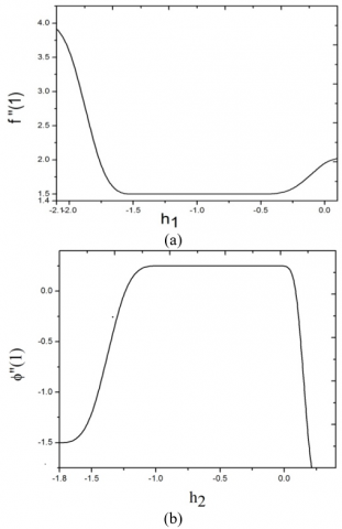
The velocity and concentration distributions involve auxiliary parameters h1 and h2. Convergence rate for the homotopy approximations strongly taking the value of h [26]. As a result, h-curves are depicted for finding the range of h1 and h2. The h-curves are depicted in Figures 2(a)–2(b)for 20thorder of approximation. It is obvious that h1 and h2 values have these ranges: -1.5< h1<-0.5 and -1.25< h2< 0. So we have taken h1 = h2 = -1. The enormous convergence range for the approximation of the 20th order accepted in all subsequent calculations and figures is achieved.
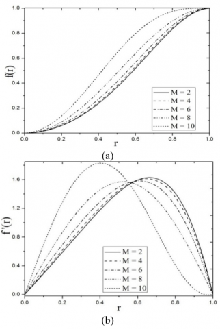
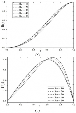
Figures 3(a)-3(b) displays the response of M on radial and axial velocity components $f \& f^{\prime}$ . These figures show that the velocity is increased with an increase in M, wherever the velocity element within the z-direction is that the most values of $f^{\prime}$ are reduced and shifted towards the origin (axis of the cylinder) with the increasing values of M. The Lorentzian forces are responsible for the velocity coefficients in (r, z) directions. The radial component assists momentum development and enhances the flow in r-direction. The Lorentzian magnetic force along axis of pipe acts to inhibit flow, especially at larger values of the radial coordinate. It is clear from Figure 4(a) that the velocity f increases as Re increases. From Figure 4(b), we see that the highest values of M are reduced as Re enhances. This observation is against the effect of M which enhances the maximum values of $f^{\prime}$ . This may be due to the fact Reynolds number implies a greater inertial force in the regime relative to viscous force and this handle to accelerate the flow along r-axis. Re cannot induce a force in the perpendicular direction as in the case of magnetic parameter M.
Figure 2. $h$ curves for a ) velocity with $M=5, R e=10$ b) Concentration $\phi(\mathrm{r})$ at $M=5, R e=10, S c=0.7, K_{1}=0.1, y=1, N=2, z=1$
Figure 3. Response of $M$ on a) Radial velocity(f) with $R e=10, \mathcal{N}=2, z=1$ b) Axial velocity $\left(f^{\prime}\right)$ with $R e=10, \mathcal{N}=2, z=1$
Figure 4. Responce of $R e$ on a ) Radial velocity with $\left.M=3, N=2, z=1 ; \text { b }\right)$ Axial velocity with $M=3, N=2, z=1$
Figure 5. Responce of Re on a) Axial Concentration with $M=1, r=0.75, S c=0.5, \gamma=0.3, K_{1}=0.1$ b) Radial Concentration with at $M=I, z=1.75, S c=0.5, \gamma=0.3, K_{l}=0.1$
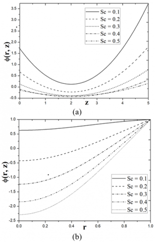
Figure 6. Effect of Sc on a) Axial Concentration with $M=4, r=0.25, R e=10, \gamma=1, K_{1}=0.1$ b) Radial Concentration with at $M=1, z=0.75, R e=10, \gamma=1, K_{l}=0.1$
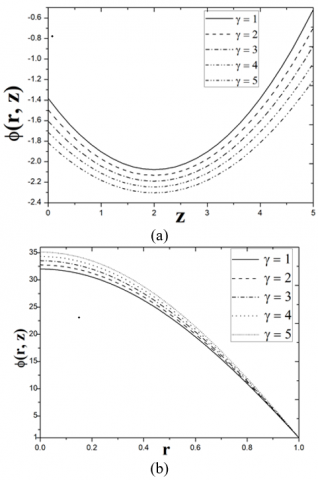
Figure 7. Effect of $\gamma$ on a) Axial Concentration with $M=4, r=0.5, R e=10, \mathrm{Sc}=0.7, K_{1}=0.1$ b) Radial Concentration with at $M=1, z=1.5, R e=10, \mathrm{Sc}=1, K_{l}=0.1$
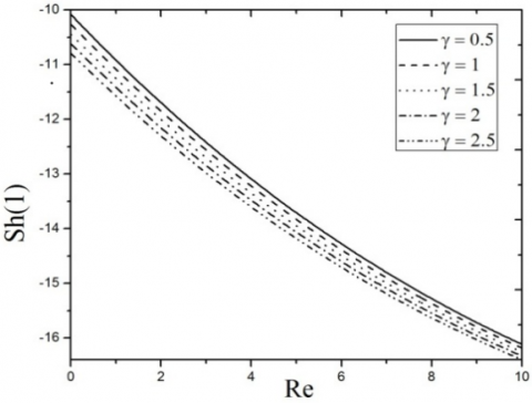
Figure 8. Sherwood distribution: Effect of γ when K1=0.15, N=2, r=1, M=1, Re=5, Sc=0.25
Figures $5(a)-5(b)$ demonstrate the response of $R e$ on axial and radial concentration $\phi .$ Practically shows that for a given rise in Re the axial and radial concentration $\phi$ numerically increases. But as $z$ increases $\phi$ decreases initially upto $z=1.2$ then $\phi$ increases. Figures $6(a)-6(b)$ illustrate the deviation of Schmidt parameter $S c$ on axial and radial concentration $\phi .$ t is observed that $\phi$ decelerates for a given enhance in $S c$ (i.e., with declining of molecular diffusivity). This is due to the fact that the molecular diffusivity develops into relatively less momentum as $S c$ is enchanted. The effect of first order reaction parameter $\gamma$ on dimensionless axial and radial concentration distribution $\phi$ is shown in Figures $7(\mathrm{a})$ to $7(\mathrm{b})$ The rate of reaction is the speed at which reactants are changed into products. It is experiential that for the case of axial \phidecelerates for a given enhance in $\gamma .$ Additionally, the behavior is inverted the radial concentration $\phi$ increases as $\gamma$ increases. Figure 8 represents the Sherwood distribution $S h$ versus Re for different values of $\gamma .$ It presents the proportion of the convective mass transportation to the rate of diffusive mass transfer. From this figure, it is observed that $S h$ decelerates as $\gamma$ raises.
4.1 Streamlines and contours of concentration
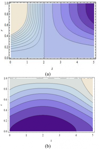
From the picture $9(\text { a ) Streamlines for } z \leq N$ are positive and non-positive for $z>N$ are detected. The streamlines of line $z$ $=N$ are demographically symmetric. The streamlines are more clustered for lower $z$ values and more dispersed for greater $z$ values indicating that the intensity of the flow is greater at lower $z$ (axial coordinate). From the picture $9(b),$ the concentration around line $z=N$ is symmetrical to almost $r=$ $0.5 .$ The concentration is minimal near the axis of the cylinder (because gradual blue shading is present in that region). At $z$ $=N$ and $r=0,$ the lowest concentration appears.
Figure 9. a) Stream lines for velocity at Re $=10, M=2, S c=0.7, \gamma=1, K_{1}=0.2 ;$ b ) Contour graphs for Concentration at Re $=10, M=2, S c=0.7, \gamma=1, K_{1}=0.2$
Analytical solutions are given for the Mass transfer in Newtonian MHD pipe flow exploitation the homotopy analysis technique (HAM). Wall suction/injection and first order chemical reaction effects are also included. The following conclusions were made
(i) Increasing the magnetic force parameter strongly retards the axial flow, although it accelerates the radial flow.
(ii) Increasing the number of suction Reynolds slows the axial velocity and rises the radial velocity.
(iii) The non-dimensional concentration $\phi$ decelerates for $\gamma>0 .$ Additionally, $\phi$ decelerates as such Sc rises. In the absence of an expanding/contracting parameter, these investigations are qualitatively consistent with the results of Srinivas et al. [ 23]
(iv) The Sherwood number decline with chemical reaction parameter $\gamma$ increments.
The authors are grateful to the anonymous referees for remarks which improved the work considerably.
|
W, U |
dimensional axial and radial velocity components |
|
w, u |
non-dimensional axial and radial velocity components |
|
p, P |
non-dimensional and dimensional pressure |
|
D |
Diffusion coefficient |
|
C |
Concentration of the fluid |
|
E2 |
Stoke’s stream function operator |
|
$N=U_{a} / v_{0}$ |
|
|
v0 |
suction velocity |
|
U0 |
entrance velocity |
|
k1 |
chemical reaction rate. |
|
C0 |
reference concentration at the axis |
|
Cw |
wall concentration at the surface of pipe |
|
Re |
Suction Reynolds number |
|
M |
Magnetic parameter |
|
Sc |
Schmidt number |
|
Greek symbols |
|
|
$\rho$ |
density |
|
$\mu$ |
Viscosity kg. m-1.s-1 |
|
$\sigma$ |
electrical conductivity |
|
$\phi$ |
Dimensionless concentration |
|
$\gamma$ |
Chemical reaction parameter |
[1] Berman, A.S. (1953). Laminar flow in channels with porous walls. Journal of Applied Physics, 24(9): 1232-1235. http://dx.doi.org/10.1063/1.1721476
[2] Sellars, J.R. (1955). Laminar flow in channels with porous walls at high suction Reynolds numbers. Journal of Applied Physics, 6(4): 489. http://dx.doi.org/10.1063/1.1722024
[3] Yuan, S.W. (1956). Further investigation of laminar flow in channels with porous walls. Journal of Applied Physics, 27(3): 267-269. http://dx.doi.org/10.1063/1.1722355
[4] Bansal, J.L. (1967). Laminar flow through a uniform circular pipe with small suction. Proc. Natn. Acad. Sci. 32A(4): 368-378.
[5] Terril, R.M. (1982). An exact solution for flow in a porous pipe. Zeitschrift für angewandte Mathematik und Physik, 33: 547-542. https://doi.org/10.1007/BF00955703
[6] Terril, R.M. (1983). Laminar flow through a porous tube. J. Fluids Eng., 105(3): 303-306. https://doi.org/10.1115/1.3240992
[7] Tsangaris, S., Kondaxakis, D. (2007). Exact solution for flow in a porous pipe with unsteady wall suction/injection. Comm. in Nonlinear Sci. Num. Simu., 12(7): 1181-1189. https://doi.org/10.1016/j.cnsns.2005.12.009
[8] Cox, B.J., Hill, J.M. (2011). Flow through a circular tube with permeable Navier slip boundary. Nanoscale Research Letters, 389: 1-9. https://doi.org/10.1186/1556-276X-6-389
[9] Ramana Murthy, J.V., Nagaraju, G., Muthu, P. (2012). Micropolar fluid flow generated by a circular cylinder subject to longitudinal and torsional oscillations with suction/injection. Tamkang J. Mathematics, 43(3): 339-356. https://dx.doi.org/10.5556/j.tkjm.43.2012.339-356
[10] Srinivas, J., Ramana Murthy, J.V. (2016). Flow of two immiscible couple stress fluids between two permeable beds. J. Applied Fluid Mechanics, 9(1): 501-507. https://dx.doi.org/10.5556/j.tkjm.43.2012.339-356
[11] Terril, R.M., Shrestha, G.M. (1963). Laminar flow through channels with porous walls and with an applied transverse magnetic field. Appl. Sci. Res., 11: 134-144. https://dx.doi.org/10.1007/BF02922219
[12] Attia, H.A. (2003). Unsteady flow of a dusty conducting non-Newtonian fluid through a pipe. Can. J. Phys., 81(5): 789-795. https://dx.doi.org/10.1139/p03-054
[13] Attia, H.A., Ahmed, M.E.S. (2005). Circular pipe MHD flow of a dusty Bingham fluid. Tamkang J. Science and Engineering, 8(4): 257-265.
[14] EL-Shahed, M. (2006). MHD of a fractional viscoelastic fluid in a circular tube. Mech. Res. Comm., 33: 261-268. https://dx.doi.org/10.1016/j.mechrescom.2005.02.017
[15] Ramana Murthy, J.V., Bahali, N.K., Srinivasacharya, D. (2010). Unsteady flow of a micropolar fluid through acircular pipe under a transverse magnetic field with suction/injection. Selguk Journal of Applied Mathematics, 11(2): 13-25.
[16] Ramana Murthy, J.V., Sai, K.S., Bahali, N.K. (2011). Steady flow of micropolar fluid in a rectangular channel under transverse magnetic field with suction. AIP Advances, 1(032123). https://doi.org/10.1063/1.3624837
[17] Hayat, T., Abbas, Z. (2008). Channel flow of a Maxwell fluid with chemical reaction. Z Angew Math Phys., 59: 124-144. https://dx.doi.org/10.1007/s00033-007-6067-1
[18] Bridges, C., Rajagopal, K.R. (2006). Pulsatile flow of a chemically-reacting nonlinear fluid. Comput Math Appl., 52(6-7): 1131-1144. https://dx.doi.org/10.1016/j.camwa.2006.01.014
[19] El Dabe, N.T., Moatimid, G.M., Ali, H.S.M. (2002). Rivlin-Eriksen fluid in tube of varying cross section with mass and heat transfer. Z. Naturforsch. 57(11): 863-873. https://doi.org/10.1515/zna-2002-1105
[20] Sahin, A.Z., Ben-Mansour, R. (2003). Entropy generation in laminar fluid flow through a circular pipe. Entropy, 5(5): 404-416. https://dx.doi.org/10.3390/e5050404
[21] Ben-Mansour, R., Sahin, A.Z. (2005). Entropy generation in developing laminar fluid flow through a circular pipe with variable properties. Heat Mass Transfer, 42: 1-11. https://dx.doi.org/10.1007/s00231-005-0637-6
[22] Ramana Murthy, J.V., Nagaraju, G., Sai, K.S. (2012). Numerical solution for MHD flow of micro polar fluid between two concentric rotating cylinders with porous lining. International Journal of Nonlinear Science, 13(2): 183-193.
[23] Srinivas, S., Subramanyam Reddy, A., Ramamohan, T.R. (2015). Mass transfer effects on viscous flow in an expanding or contracting porous pipe with chemical reaction. Heat Transfer-Asian Research, 44(6): 552-567. https://dx.doi.org/10.1002/htj.21136
[24] Mandapati, M.J.K. (2016). Effect of axial conduction and viscousdissipation on heat transfer for laminarflow through a circular pipe. Perspectives in Science, 8: 61-65. https://dx.doi.org/10.1016/j.pisc.2016.03.008
[25] Nagaraju, G., Srinivas, J., Ramana Murthy, J.V., Rashad, A.M. (2017). Entropy generation analysis of the mhd flow of couple stress fluid between two concentric rotating cylinders with porous lining. Heat Transfer-Asian Research, 46(4): 316-330. https://dx.doi.org/10.1002/htj.21214
[26] Gajjela, N., Matta, A., Kaladhar, K. (2017). The effects of Soret and Dufour, chemical reaction, Hall and ion currents on magnetized micropolar flow through co-rotating cylinders. AIP Advances, 7(115201): 1-16. https://dx.doi.org/10.1063/1.4991442
[27] Bouras, A., Taloub, D., Djezzar, M., Driss, Z. (2018). Natural convective heat transfer from a heated horizontal elliptical cylinder to its coaxial square enclosure. Mathematical Modeling of Engineering Problems, 5(4): 379-385. https://dx.doi.org/10.18280/mmep.050415
[28] Nagaraju, G., Jangili, S., Murthy, R.J.V., Beg, O.A., Kadir, A. (2019). Second law analysis of flow in a circular pipe with uniform suction and magnetic field effects. J of Heat Transfer, 141(1): 012004. https://doi.org/10.1115/1.4041796
[29] Liao, S.J. (2004). Beyond perturbation: Introduction to Homotopy analysis method. Applied Mechanics Reviews, 57(5): B25-B26. https://dx.doi.org/10.1115/1.1818689
[30] Bird, R.B., Stewart, W.E., Lightfoot, E.N. (1960). Transport Phenomena. John Wiley and Sons, New York. https://doi.org/10.1002/aic.690070245