Thriveni Kunnegowda | Basavarajappa Mahanthesh* | Giulio Lorenzini | Isaac Lare Animasaun
OPEN ACCESS
The effects of the exponential space based heat source on quadratic convective flow of Casson fluid in a microchannel with an induced magnetic field is studied through a statistical approach. The flow is considered in vertical microchannel formed by two vertical plates. The solution for the governing equations has been obtained for the velocity, induced magnetic field and temperature field using Homotopy Perturbation Method (HPM). The current density, skin friction co-efficient and Nusselt number expressions are also estimated. The impact of various physical parameters on the velocity, temperature, induced magnetic field, current density, skin friction co-efficient and Nusselt number distributions have been discussed with the help of graphs. The results obtained by using HPM, are compared to those obtained by using the Runge-Kutta-Fehlberg 4-5th order method and an excellent agreement is found. The impact of Casson fluid parameter and the exponential heat source is qualitatively agreed for all flow fields.
Casson fluid, exponential heat source, microchannel, nonlinear convection, nonlinear boussinesq approximation
The heating/cooling applications at engineering require high thermal performance to the thermal systems. As a result, it has attracted many researchers to find the technique to enhance the rate of heat transfer in the cooling and thermal engineering system. However, the enhancement of thermal energy is one of the challenges in these applications. The significant of the heat transfer enhancement can be obtained by developing compact devices that are small in size, reduction in equipment weight or light weight and having high efficiency. The transfer of energy due to the temperature difference is termed as a heat exchanger. In the field of energy conservation, conversion and recovery heat exchangers play a very important role. The heat exchanger can be found and used in many applications such as household air conditioning, automotive air conditioning system and manufacturing processes. In view of this, in 1981 Tuckerman and Pease [1] proposed a micro-channel heat exchanger for the first time. Later, Mehendale defined the micro-channel heat exchanger as hydraulic diameter less than 1mm. The heat exchange between two different fluids in a microchannel was first developed by Swift [2] in the year 1985. The natural convection in an open-ended micro-channel was investigated analytically by Chen and Weng [3]. They found that in the slip-flow natural convection, rarefaction and fluid-wall interaction have significant effects on the flow. Taking suction/injection effect into account, later this work was extended by Jha et al. [4]. They concluded that skin friction coefficient and rate of heat transfer strongly depend on suction/injection parameter. Wang and Chiu-On [5] investigated the natural convection in a vertical microchannel influenced by no-slip condition. The main conclusion drawn from these studies is that the heat transfer enhancement can be done by accounting the micro-channel.
The above studies are concerned with natural convection involving various physical parameters like MHD, suction/injection velocity slip condition wherein linear Boussinesq approximation has been taken into account. Since density is directly proportional to the temperature/concentration difference as the temperature difference increases it is possible to have a nonlinearity fluctuation in the density which will affect the flow fields consequently. The nonlinear density variation with temperature was proposed by Vajravelu et al. [6] and is as follows
$\rho(T)=\rho\left(T_{0}\right)+\left(\frac{\partial \rho}{\partial T}\right)_{0}\left(T-T_{0}\right)+\frac{1}{2}\left(\frac{\partial^{2} \rho}{\partial T^{2}}\right)_{0}\left(T-T_{0}\right)^{2}+\cdots$
By following Vajravelu et al. [6], the three dimensional analysis of radiation and nonlinear convection for the flow of a non-Newtonian nanofluid was studied by Mahanthesh et al. [7]. They found that the temperature profile is stronger in the case of solar radiation. Hayat et al. [8] studied the effect of nonlinear convection in thixotropic fluid with magnetic field. Nonlinear convection of third grade fluid on stratified flow was investigated by Waqas et al. [9]. Gireesha et al. [10] studied the nonlinear convective flow of nanoliquid subjected to an exponential heat source and variable viscosity. However, the amount of literature done on nonlinear convection using microchannel is limited. Thus, this study is proposed to fill this gap in the literature.
The Newtonian theory fails to explain the characteristics of many materials like paint, shampoos, printing ink, tomato paste, etc., so the non-Newtonian theory was introduced. Among them, Casson liquid exhibits the stress, shear thinning characteristics along with high shear viscosity. The Casson fluid model was first introduced by Casson in the year 1959 which describes the flow of viscoelastic fluids. Many researchers showed their interest to study the Casson fluid model due to the variety of applications of Casson fluid in the field of petrochemical, food processing and in the field of metallurgy, etc. The flow of Casson fluid over a stretching cylinder by considering magnetism was studied by Tamoor et al. [11]. Later, the numerical study on magneto Casson fluid with cross-diffusion effect was investigated by Pushpalatha et al. [12]. MHD flow of Casson fluid through porous microchannel subjected to thermal radiation was examined by Shashikumar et al. [13]. Makinde et al. [14-15] addressed the combined effect of thermal radiation, suction/injection, magnetic field and porous media in the forced convection flow of an electrically conducting Casson fluid in a horizontal and vertical microchannel with velocity slip and temperature jump condition.
Magnetohydrodynamics deals with the movement of particles influenced by electromagnetic field. It is mainly focused on the particles in which currents are induced by induction. The novelty behind magnetohydrodynamics is that current in a moving convective field can be induced by a magnetic field. The induced magnetic field plays a significant role in the case of nuclear reactors, thermomagneto aerodynamics etc. The significance of induced magnetic field on natural convection in a vertical microchannel was investigated by Basant et al. [16]. Shivakumar et al. [17] studied the influence of induced magnetic field on the forced convection subjected to magnetic field. The role of induced magnetic field on a mixed convection flow in microchannel was addressed by Basant et al. [18]. In view of these, the study on transport of Casson fluid under nonlinear Boussinesq approximation in a microchannel in presence of induced magnetic field and exponential heat source is an open question. Therefore, the prime purpose of this study is to investigate the momentum and thermal behavior of Casson fluid in the presence of the induced magnetic field, exponential heat source under nonlinear Boussinesq approximation in a microchannel. The governing equations are treated analytically by using HPM under velocity slip and temperature jump boundary conditions. The following section illustrates the basic idea of HPM.
To explain the basic idea of HPM, consider the nonlinear differential equation of the form (see [19-20]):
$A(u)-f(l)=0, l \in D$ (1)
with the boundary condition:
$B\left(u, \frac{\partial u}{\partial m}\right)=0, l \in F$ (2)
where A, B, f(l) and F are general differential operator, boundary operator, a known analytical function and boundary of the domain D respectively. The operator A can be divided into linear(L) and nonlinear(L) parts. Therefore Eq. (1) can be written as:
$L(u)+N(u)-f(l)=0, l \in D$ (3)
The HPM structure can be written as:
$H(v, p)=(1-p)\left[L(v)-L\left(u_{0}\right)\right]+p[A(v)-f(l)]=0$ (4)
where
$v(l, p) : D \times[0,1] \rightarrow R$
In Eq. (4), $p \in[0,1]$ is an embedding parameter, while $u_{0}$ is an initial approximation that satisfies the boundary condition. The solution for the Eq. (4) can be expressed as a power series in P, as follows:
$v=v_{0}+p v_{1}+p^{2} v_{2}+\ldots$ (5)
setting p=1 gives the approximate solution of Eq. (1) as
$u=\lim _{p \rightarrow 1} v=v_{0}+v_{1}+v_{2}+\ldots$ (6)
The physical configuration of the problem consisting of two infinite vertical plates which are separated by a distance b is as shown in Figure 1. The quadratic convective flow of Casson fluid with exponential heat source is considered in a vertical microchannel. The flow is assumed to be non-transient, unidirectional. A coordinate system is considered in such a way that x'-axis is opposite to gravity and y'-axis is perpendicular to the vertical microchannel. The plates are heated asymmetrically with left plate is maintained at a temperature T2 and the right plate at a temperature T2 with T1>T2. Therefore, there exists a large temperature difference between the plates causing nonlinear convection in the microchannel.
Figure 1. Physical arrangement of the problem
Using nonlinear Boussinesq’s approximation the governing equations of momentum, magnetic field and energy are given below (see [16]):
$\left(1+\frac{1}{\beta}\right)\left(\frac{d^{2} u^{\prime}}{d y^{2}}\right)+\left(\frac{\mu_{e} H_{0}^{\prime}}{\rho}\right)\left(\frac{d H_{x}}{d y}\right)+g\left[\beta_{0}\left(T^{\prime}-T_{0}\right)+\beta_{1}\left(T^{\prime}-T_{0}\right)^{2}\right]=0$ (7)
$\frac{1}{\beta \mu_{e}}\left(\frac{d^{2} H_{x}^{\prime}}{d y^{\prime 2}}\right)+H_{0}^{\prime}\left(\frac{d u^{\prime}}{d y^{\prime}}\right)=0$ (8)
$k \frac{d^{2} T^{\prime}}{d y^{\prime 2}}+q_{e}\left(T_{1}-T_{0}\right) \exp \left(\frac{-n y^{\prime}}{b}\right)=0$ (9)
$u^{\prime}\left(y^{\prime}\right)=\frac{2-\sigma_{v}}{\sigma_{v}} \lambda\left(\frac{d u}{d y}\right), H_{x}^{\prime}\left(y^{\prime}\right)=0$
$T^{\prime}\left(y^{\prime}\right)=T_{2}+\frac{2-\sigma_{t}}{\sigma_{t}}\left(\frac{2 v}{v+1}\right)\left(\frac{\lambda}{\operatorname{Pr}}\right)\left(\frac{d T^{\prime}}{d y^{\prime}}\right)$ at $y^{\prime}=0$ (10)
$u^{\prime}\left(y^{\prime}\right)=-\frac{2-\sigma_{\nu}}{\sigma_{\nu}} \lambda\left(\frac{d u}{d y}\right), H_{x}^{\prime}\left(y^{\prime}\right)=0$
$T^{\prime}\left(y^{\prime}\right)=T_{1}-\frac{2-\sigma_{t}}{\sigma_{t}}\left(\frac{2 v}{v+1}\right)\left(\frac{\lambda}{\operatorname{Pr}}\right)\left(\frac{d T^{\prime}}{d y^{\prime}}\right)$ at $y^{\prime}=b$ (11)
where all the symbols are defined in the nomenclature section.
Now introducing the following non-dimensional quantities (see [16])
$y=\frac{y^{\prime}}{b}, u=\left(\frac{v u^{\prime}}{g \beta_{0} b^{2}\left(T_{1}-T_{0}\right)}\right), \theta=\frac{T^{\prime}-T_{0}}{T_{1}-T_{0}}, P m=v \sigma \mu_{e}$
$\alpha=\frac{\beta_{1}}{\beta_{0}}\left(T_{1}-T_{0}\right), Q=\frac{q_{e} b^{2}}{k}, M=\frac{H_{0}^{\prime} b}{v} \sqrt{\frac{\mu_{e}}{\rho}}$
$H=\frac{v H_{x}^{\prime}}{g \beta b^{2}\left(T_{1}-T_{0}\right)} \sqrt{\frac{\mu_{e}}{\rho}}$
into the governing Eqns. (7)-(9) and boundary conditions (10) and (11) then one can get:
$\left(1+\frac{1}{\beta}\right)\left(\frac{d^{2} u}{d y^{2}}\right)+M\left(\frac{d H}{d y}\right)+\theta+\alpha \theta^{2}=0$ (12)
$\frac{d^{2} H}{d y^{2}}+M P m\left(\frac{d u}{d y}\right)=0$ (13)
$\frac{d^{2} \theta}{d y^{2}}+Q \exp (-n y)=0$ (14)
$u(y)=\beta_{v} K n\left(\frac{d u}{d y}\right), H(y)=0, \theta(y)=\xi+\beta_{v} K n \ln \left(\frac{d \theta}{d y}\right)$ at $y=0$ (15)
$u(y)=-\beta_{v} K \eta\left(\frac{d u}{d y}\right), H(y)=0, \theta(y)=1-\beta_{v} K n \ln \left(\frac{d \theta}{d y}\right)$ at $y=1$ (16)
On constructing a convex Homotopy on Eqns. (12)-(14) and applying the HPM to solve the governing equations one can have:
$H(u, p)=(1-p)\left(1+\frac{1}{\beta}\right) u^{\prime \prime}+p\left[\left(1+\frac{1}{\beta}\right) u^{\prime \prime}+M H^{\prime}+\theta+\alpha \theta^{2}\right]=0$ (17)
$H(H, p)=(1-p) H^{\prime \prime}+p\left\lfloor H^{\prime \prime}+M P m \dot{u}\right\rfloor= 0$ (18)
$H(\theta, p)=(1-p) \theta^{\prime \prime}+p\left|\theta^{\prime \prime}+Q e^{-n y}\right|=0$ (19)
Assuming the solutions of Eqns. (12)-(14) to be written as
$\begin{aligned} u &=\mathrm{u}_{0}+p \mathrm{u}_{1}+p^{2} \mathrm{u}_{2}+\ldots \\ \mathrm{H} &=\mathrm{H}_{0}+p \mathrm{H}_{1}+p^{2} \mathrm{H}_{2}+\ldots \\ u=& \theta_{0}+p \theta_{1}+p^{2} \theta_{2}+\ldots \end{aligned}$ (20)
Substituting Eq. (20) into Eqns. (17)-(19) and simplifying, one can get
$\left(1+\frac{1}{\beta}\right)\left[u_{0}^{\prime \prime}+p u_{1}^{\prime \prime}+p^{2} u_{2}^{\prime \prime}+p^{3} u_{3}^{\prime \prime}+\ldots\right]+p\left[M\left(H_{0}^{\prime}+p H_{1}^{\prime}+p^{2} H_{2}^{\prime}+p^{3} H_{3}^{\prime}+\ldots\right)\right.$
$\begin{aligned}+\left(\theta_{0}+p \theta_{1}+p^{2} \theta_{2}+p^{3} \theta_{3}+\ldots\right) &+\alpha\left(\theta_{0}^{2}+2 p \theta_{0} \theta_{1}+p^{2}\left(2 \theta_{0} \theta_{2}+\theta_{1}^{2}\right)\right.\\ &\left.\left.+p^{3}\left(2 \theta_{0} \theta_{3}+2 \theta_{1} \theta_{2}\right)+\ldots\right)\right]=0 \end{aligned}$ (21)
$\begin{aligned}\left(H_{0}^{\prime \prime}+p H_{1}^{\prime \prime}+p^{2} H_{2}^{\prime \prime}+p^{3} H_{3}^{\prime \prime}\right.&+\ldots)+p M P m\left(u_{0}^{\prime}+p u_{1}^{\prime}\right.\\ &\left.+p^{2} u_{2}^{\prime}+p^{3} u_{3}^{\prime}+\ldots\right)=0 \end{aligned}$ (22)
$\left(\theta_{0}^{\prime \prime}+p \theta_{1}^{\prime \prime}+p^{2} \theta_{2}^{\prime \prime}+p^{3} \theta_{3}^{\prime \prime}+\ldots\right)+p Q e^{-n y}=0$ (23)
By comparing the coefficient of $p^{0}, p^{1}, p^{2}$ and $p^{3}$ of Eqns. (21)-(23) one can have
$p^{0} : u_{0}^{\prime \prime}=0$ (24)
$H_{0}^{\prime \prime}=0$ (25)
$\theta_{0}^{\prime \prime}=0$ (26)
$p^{1} :\left(1+\frac{1}{\beta}\right) u_{1}^{\prime \prime}+M H_{0}^{\prime}+\alpha \theta_{0}^{2}+\theta_{0}=0$ (27)
$H_{1}^{\prime \prime}+M P m u_{0}^{\prime}=0$ (28)
$\theta_{1}^{\prime \prime}+Q e^{-n y}=0$ (29)
$p^{2} :\left(1+\frac{1}{\beta}\right) u_{2}^{\prime \prime}+M H_{1}^{\prime}+\theta_{1}+2 \alpha \theta_{0} \theta_{1}=0$ (30)
$H_{2}^{\prime \prime}+M P m u_{1}^{\prime}=0$ (31)
$\theta_{2}^{\prime \prime}=0$ (32)
$p^{3} :\left(1+\frac{1}{\beta}\right) u_{3}^{\prime \prime}+M H_{2}^{\prime}+\theta_{2}+2 \alpha \theta_{0} \theta_{2}+\alpha \theta_{1}^{2}=0$ (33)
$H_{3}^{\prime \prime}+M P m u_{2}^{\prime}=0$ (34)
$\theta_{3}^{\prime \prime}=0$ (35)
Subsequent boundary conditions are
$\begin{aligned} u_{i}(0) &=\beta_{v} K n u_{i}^{\prime}(0) \\ H_{i}(0)=0 & \\ \theta_{0}(0)=& \xi+\beta_{v} K n \ln \theta_{0}^{\prime}(0) \\ \theta_{j}(0)=& \beta_{v} K n \ln \theta_{j}^{\prime}(0) \\ u_{i}(1)=&-\beta_{v} K n u_{i}^{\prime}(1) \end{aligned}$
$H_{i}(1)=0$
$\theta_{0}(1)=1-\beta_{v} \operatorname{Knln} \theta_{0}^{\prime}(1)$
$\theta_{j}(1)=-\beta_{v} K n \ln \theta_{j}^{\prime}(1)$
where, $i=0,1,2, \ldots$ and $j=1,2,3, \ldots$ (36)
Upon solving, above system one can have
$u_{0}=0, H_{0}=0$ (37)
$\theta_{0}=c_{1} y+c_{2}$ (38)
$u_{1}=-\left(1+\frac{1}{\beta}\right)^{-1}\left[\begin{array}{c}{\frac{c_{1} y^{3}}{6}\left(1+\frac{\alpha c_{1} y}{2}\right)+\left(\frac{c_{2} y^{2}}{2}\right)\left(1+\alpha c_{2}\right)} \\ {+\left(\frac{\alpha c_{1} c_{2} y^{3}}{3}\right)+a_{3} y+a_{4}}\end{array}\right]$ (39)
$H_{1}=0$ (40)
$\theta_{1}=c_{5} y+c_{6}-\left(\frac{Q e^{-n y}}{n^{2}}\right)$ (41)
$H_{2}=\frac{M P m}{\left(1+\frac{1}{\beta}\right)}\left[\begin{array}{c}{\frac{c_{1} y^{4}}{12}\left(\frac{c_{1} \alpha y}{5}+\frac{1}{2}\right)+\frac{c_{2} y^{3}}{6}\left(1+\alpha c_{2}\right)} \\ {+\frac{\alpha c_{1} c_{2} y^{4}}{12}+\frac{a_{3} y^{2}}{2}}\end{array}\right]-b_{5} y-b_{6}$ (43)
$\theta_{2}=c_{3} y+c_{4}$ (44)
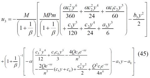
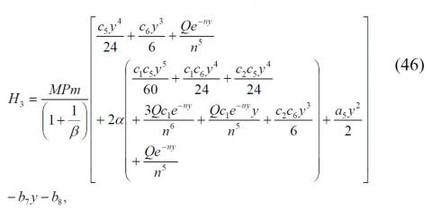
${{\theta }_{3}}={{c}_{7}}y+{{c}_{8}}.$ (47)
The approximate solution for the velocity, induced magnetic field and temperature can be obtained from the Eqns. (37)-(47) as
$u={{u}_{0}}+{{u}_{1}}+{{u}_{2}}+{{u}_{3}}+...,$ (48)
$H={{H}_{0}}+{{H}_{1}}+{{H}_{2}}+{{H}_{3}}+...,$ (49)
$\theta ={{\theta }_{0}}+{{\theta }_{1}}+{{\theta }_{2}}+{{\theta }_{3}}+...,$ (50)
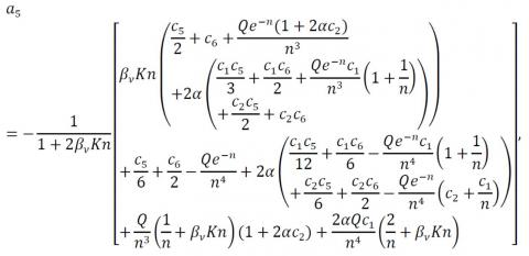
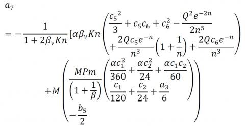
where,
$\begin{align} & {{a}_{1}}={{a}_{2}}={{b}_{1}}={{b}_{2}}={{b}_{3}}={{b}_{4}}={{b}_{6}}={{c}_{3}} \\ & ={{c}_{4}}={{c}_{7}}={{c}_{8}}=0,{{a}_{4}}={{\beta }_{\nu }}Kn{{a}_{3}}, \\\end{align}$
${{a}_{3}}=-\frac{1}{1+2{{\beta }_{\nu }}Kn}\left[ \begin{align} & {{c}_{1}}\left( \frac{{{\beta }_{\nu }}Kn}{2}+\frac{{{c}_{1}}\alpha {{\beta }_{\nu }}Kn}{3}+\frac{1}{6}+\frac{\alpha {{c}_{1}}}{12} \right) \\ & +{{c}_{2}}\left( {{\beta }_{\nu }}Kn(1+\alpha {{c}_{2}})+\frac{1+\alpha {{c}_{2}}}{2} \right) \\ & +\alpha {{c}_{1}}{{c}_{2}}\left( \frac{1}{3}+{{\beta }_{\nu }}Kn \right) \\\end{align} \right],$
${{a}_{6}}=\frac{Q}{{{n}^{3}}}\left( \frac{1}{n}+{{\beta }_{\nu }}Kn \right)(1+2\alpha {{c}_{2}})+\frac{2\alpha Q{{c}_{1}}}{{{n}^{4}}}\left( \frac{2}{n}+{{\beta }_{\nu }}Kn \right)+{{a}_{5}}{{\beta }_{\nu }}Kn,$
$\begin{align} & {{a}_{8}}={{\beta }_{\nu }}Kn\alpha \left( \frac{2Q}{{{n}^{3}}}\left( \frac{{{c}_{5}}}{n}+{{c}_{6}}-\frac{Q}{4{{n}^{2}}} \right) \right) \\ & -\alpha \left( \frac{2Q}{{{n}^{4}}}\left( -\frac{2{{c}_{5}}}{n}-{{c}_{6}}+\frac{Q}{8{{n}^{2}}} \right) \right)+{{\beta }_{\nu }}Kn{{a}_{7}}, \\\end{align}$
${{b}_{5}}=MPm{{\left( 1+\frac{1}{\beta } \right)}^{-1}}\left( \frac{\alpha c_{1}^{2}}{60}+\frac{\alpha c_{2}^{2}}{6}+\frac{\alpha {{c}_{1}}{{c}_{2}}}{12}+\frac{{{c}_{1}}}{24}+\frac{{{c}_{2}}}{6}+\frac{{{a}_{3}}}{2} \right),$
${{b}_{8}}=MPm{{\left( 1+\frac{1}{\beta } \right)}^{-1}}\left( \frac{Q}{{{n}^{5}}}+2\alpha \left( \frac{3Q{{c}_{1}}}{{{n}^{6}}}+\frac{Q{{c}_{2}}}{{{n}^{5}}} \right) \right),$
${{c}_{1}}=\frac{1-\xi }{1+2{{\beta }_{\nu }}Kn\ln },{{c}_{2}}=\xi +{{c}_{1}}{{\beta }_{\nu }}Kn\ln ,$
${{c}_{5}}=\frac{Q}{(1+2{{\beta }_{\nu }}Kn\ln )n}\left( \frac{{{e}^{-n}}-1}{n}-{{\beta }_{\nu }}Kn\ln ({{e}^{-n}}+1) \right),$${{c}_{6}}=\frac{Q}{n}\left( \frac{1}{n}+{{\beta }_{\nu }}Kn\ln \right)+{{c}_{5}}{{\beta }_{\nu }}Kn\ln .$
The induced current density can be found by:
$J=-\frac{dH}{dy}$ (51)
The volume flow rate (Qm) in dimensionless is given by:
${{Q}_{m}}=\int\limits_{0}^{1}{u(y)dy}$ (53)
From Eq. (48) the skin friction co-efficient at y=0 and y=1 in nondimensional form can be obtained as (see [16]):
${{\tau }_{0}}={{\left( \frac{du}{dy} \right)}_{y=0}}$, (55)
$=-{{\left( 1+\frac{1}{\beta } \right)}^{-1}}\left[ \begin{align} & {{a}_{3}}+{{a}_{5}}+{{a}_{7}}+\frac{Q}{{{n}^{3}}}\left( 1-\frac{\sigma Q}{2{{n}^{2}}} \right) \\ & +\frac{2\alpha Q}{{{n}^{3}}}\left( {{c}_{2}}+{{c}_{6}}+\frac{1}{n}({{c}_{1}}+{{c}_{5}}) \right) \\\end{align} \right].$ (56)
${{\tau }_{1}}={{\left( \frac{du}{dy} \right)}_{y=1}}$, (57)
Similarly, the Nusselt number is given below (see [16])
$N{{u}_{0}}={{\left( \frac{d\theta }{dy} \right)}_{y=0}}$, (59)
$={{c}_{1}}+{{c}_{5}}+\frac{Q}{n}.$ (60)
$N{{u}_{1}}={{\left( \frac{d\theta }{dy} \right)}_{y=1}}$, (61)
$={{c}_{1}}+{{c}_{5}}+\frac{Q{{e}^{-n}}}{n}.$ (62)
In order to validate the accuracy of the solution obtained by the Homotopy perturbation method (HPM), a direct comparison is made for the values of $\tau_{0}$ and $\tau_{1}$ obtained by HPM and Runge-Kutta-Fehlberg 4-5th order method. The comparison values are recorded in table 1 and an excellent agreement is found.
Table 1. Comparison of HPM and Runge-Kutta-Fehlberg 4-5th order method solution for skin friction coefficient when $P m=\beta=n=\alpha=0.5, \ln =1.667, M=5$ and $\xi=1$
|
Q |
$\tau_{0}$ |
$\boldsymbol{\tau}_{\mathbf{1}}$ |
||
|
|
HPM |
RKFM |
HPM |
RKFM |
|
0. 1 |
0.263314607 |
0.263299381 |
-0.263162225 -0.263177451 |
|
|
0.2 |
0.276891271 |
0.276860258 |
-0.276580954 -0.276611967 |
|
|
0.3 |
0.290729992 |
0.290682629 |
-0.290256185 -0.290303548 |
|
|
0.4 |
0.30483077 |
0.304766496 |
-0.304187919 -0.304252193 |
|
|
0.5 |
0.319193605 |
0.319111858 |
-0.318376156 -0.318457902 |
|
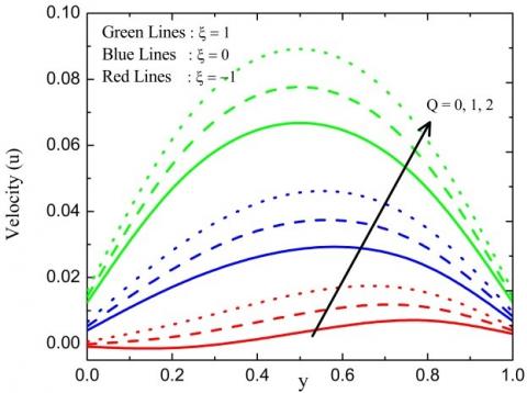
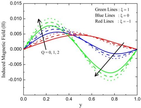
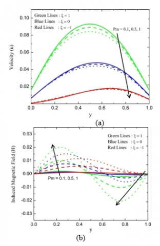
The main objective of this section is to examine the effect of exponential heat source parameter $(Q),$ induced magnetic parameter $(M),$ the magnetic Prandtl number $(P m),$ Casson parameter $(\beta),$ nonlinear convection parameter $(\alpha)$, exponential index $(n),$ Knudsen number $\left(\beta_{v} K_{n}\right)$ and fluid-wall interaction parameter (ln) on velocity $u(y),$ temperature $\theta(y),$ induced magnetic $H(y),$ induced current density $J(y),$ volume flow rate $\left(Q_{m}\right),$ skin friction co-efficient $(\tau)$ and Nusselt number $(N u)$ profiles under three case of the wall-ambient temperature difference ratio $(\xi=1 \text { for symmetrical }--$heating, $\xi=0$ for one heating and one not heating, $\xi=-1$ for one heating and one cooling). The present study has performed in the continuum and slips flow regimes $\left(K_{n} \leq\right.$ $0.1)$ . I Throught the numerical computation the other parameters are choosen as $M=5, P m=\alpha=\beta=n=$ $0.5, \beta_{v} K n=0.05, l n=1.667$ and $Q=2$ unless otherwise stated. Figure 2$(\text { a } \& \text { b ) exhibits the effect of } Q \text { and } \xi \text { on } u(y) \text { and }$ $H(y)$ when $M=5, P m=\beta=\alpha=n=0.5, \beta_{v} K_{n}=$ $0.05 \& \ln =1.667 .$ Here $Q$ and $\xi$ increases with enhancing the fluid velocity $u(y)$ and induced magnetic field $H(y),$ this is because of the contribution of more heat into the system as a result, fluid particles absorb heat and hence have a tendency as to move faster. It also observed that there exists a point of $\mathrm{f}$. intersection inside the microchannel which makes the induced magnetic field $H(y)$ to be independent of $Q$.
(a)
(b)
Figure 2. Velocity profile and induced magnetic field for different values of exponential heat source parameter Q
Figures 3 (a) and 4 (a) illustrate the effect of $M$ and $P m,$ respectively on $u(y)$ . Here as $M$ and $P m$ increases reduction in fluid velocity occurs, due to the presence of Lorentz force which is an oposing force on the velocity field. It is further noticed that in the case of asymetric heating $(\xi=-1)$ there exists a point of intersection inside the microchannel, whereas the velocity field is independent of $M$ and $P m .$ The impact of $M$ and $P m$ on the microchannel slip velocity becomes significant as $\xi$ increases. Figures 3 (b) and 4 (b) shows the variation of $M$ and $P m$ on induced magnetic field respectively. It is noticed that near the microchannel wall at $y=0$ the induced magnetic field is directly proportional to the induced magnetic parameter and the magnetic Prandtl number whereas the inverse trend is observed near the microchannel wall at $y=1 .$ In addition to this, inside the vertical microchannel there exists a point of intersection which makes the $H$ to be independent of $M$ and $P m .$ The effect of $M$ and $P m$ on the microchannel slip velocity becomes significant as $\xi$ increases.
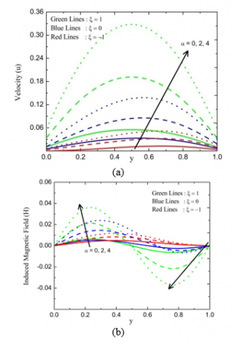
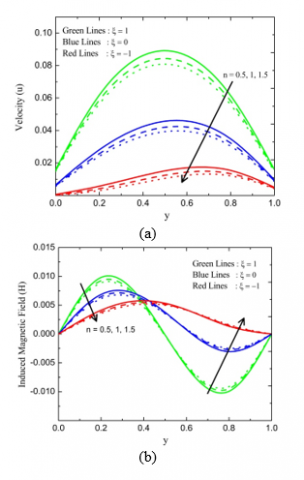
Figures 5$(\text { a } \& \text { b })$ and 6 (a $\&$ b) exhibit the effect of $\beta \& \alpha$ on $u(y)$ and $H(y)$ respectively. since $\alpha$ is directly proportional to the buoyancy force, it is found that an increase in nonlinear convection parameter leads to an increase in the velocity profile because of strong buoyancy force. Also, it is worthwhile to note that the velocity increases with $\beta$ due to the decrease in the yield stress. It is also observed that the increase in Casson fluid and nonlinear convection parameter causes an enhancement in the induced magnetic field near the microchannel wall at $y=0$ whereas reveres nature is observed at $y=1 .$ In addition to this, the induced magnetic field becomes independent of $\beta$ and $\alpha$ due to the existence point of intersection inside the vertical microchannel. Figure 7 (a \& b ) shows the effect of $n$ on $u(y)$ and $H(y) .$ It is evident that an increase in $n$ causes a reduction in both the fluid velocity and the induced magnetic field. $H(y)$ becomes independent of $n$ due to the existence of a point of intersection inside the vertical microchannel. The effect of $n$ on velocity becomes significant as $\xi$ increases.
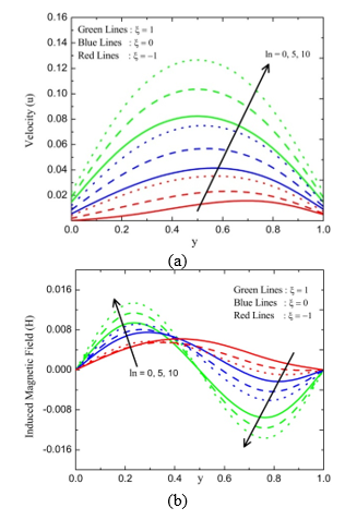
Figures 8$(a)$ and 9 (a) illustrate the effects of $\beta_{v} K_{n} \&$ ln on $u(y) .$ An increase in $\beta_{v} K_{n},$ ln $\&$ s causes an enhancement in the fluid slip and hence fluid velocity increases. Also, the fluid velocity increases with increase in the fluid-wall interaction parameter. Further, the effect of $\beta_{v} K_{n} \&$ ln on the velocity becomes significant as $\xi$ increases. Figures 8 (b) and 9 (b) exhibit the effect of $\beta_{v} K_{n} \& \ln$ on $H(y) .$ It is found that $H(y)$ increases with increases in $\beta_{v} K_{n}, \ln \& \xi$
Figure 3. Velocity profile $u(y)$ and induced magnetic field $H(y)$ for different values of induced magnetic parameter $M$
Figure 4. Velocity profile $u(y)$ and induced magnetic field $H(y)$ for different values of magnetic Prandtl number $P m$
Figure 5. Velocity profile $u(y)$ and induced magnetic field $H(y)$ for different values of Casson fluid parameter $\beta$
Figure 6. Velocity profile and induced magnetic field for different values of nonlinear convection parameter
Figure 7. Velocity profile $u(y)$ and induced magnetic field $H(y)$ for different values of exponential index $n$
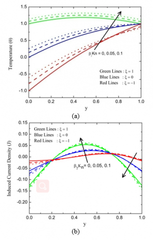
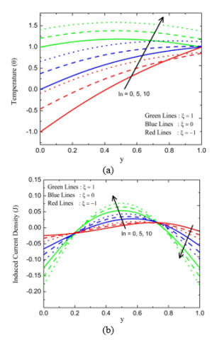
Figures 10$(\text { a } \& \text { b })$ and 11$(a \& b)$ show the effect of $Q \& n$ on $\theta(y)$ and $J(y)$ . It is observed that the temperature profile can be increased by increasing the value of heat source parameter. This is because dissipation of energy due to heat source aspect. Whereas the reduction in the temperature profile can be seen by increasing the value of $n$ . Also, a similar nature can be seen in the induced current density. Figures 12 (a) and 13 (a) present the variation of $\beta_{v} K_{n} \&$ ln on $\theta(y) .$ It is seen that, an increase in the values of $\beta_{v} K_{n}$ and $l n$ causes an enhancement in the temperature profluence of the increase in the temperature jump. The influence of $\beta_{v} K_{n}$ and $\ln$ on $\theta(y)$ becomes significant as $\xi$ increases. Figures 12 (b) and 13 (b) shows the effect of $\beta_{v} K_{n}$ and $\ln$ on $J(y) .$ It is observed that, an increase in both $\beta_{v} K_{n}$ and $l n$ causes an enhancement in $J(y)$ in the domain $y \in(0.2,0.7)$ whereas the inverse trend is seen in the domain $y \in(0,0.2)$ and $y \in(0.7,1) .$ For the wall ambient temperature difference ratio, the inverse effect of induced current density is seen. It is also found that the induced current density becomes independent of $\beta_{v} K_{n}$ and $l n$ at two points due to the existence of points of intersection inside the microchannel.
Figure 8. Velocity profile $u(y)$ and induced magnetic field $H(y)$ for different values of Knudsen number $\beta_{v} K_{n}$
Figure 9. Velocity profile $u(y)$ and induced magnetic field $H(y)$ for different values of fluid-wall interaction parameter $\ln$
Figure 10. Temperature profile $\theta(y)$ and induced current density $J(y)$ for different values of $Q$
Figure 11. Temperature profile $\theta(y)$ and induced current density $J(y)$ for different values of $n$
Figure 12. Temperature profile $\theta(y)$ and induced current density $J(y)$ for different values of $\beta_{v} K_{n}$
Figure 13. Temperature profile $\theta(y)$ and induced current density $J(y)$ for different yalues of $l n$
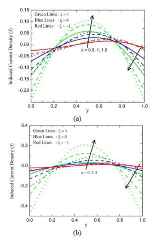
Figure 14 (a $\&$ b) shows the effect of $\beta, \alpha \& \xi$ on induced current density. Here an increase in $\beta$ and $\alpha$ causes an enhancement in the induced current density at the central region of the vertical microchannel while reveres behavior is observed at the microchannel plates. Also, it is interesting to note that current density changes its behavior at two points inside the microchannel with $\beta$ and $\alpha .$
Figure 14. Induced current density $J(y)$ for different values of $\beta$ and $\alpha$
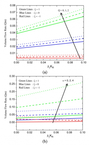
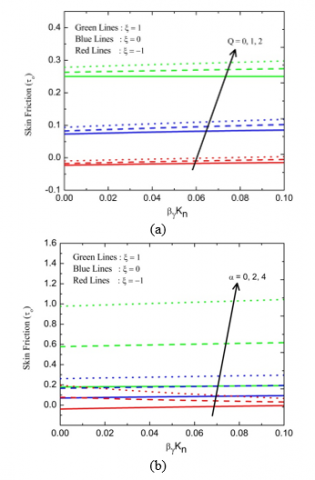
Figure 15 (a \& b) presences the variations of $Q_{m}$ with respect to $\beta_{v} K_{n}$ for different values of $Q \& \alpha$ . It is seen that an increase in $Q$ and $\alpha$ causes an enhancement in volume flow rate $\left(Q_{m}\right)$ for both symmetric and asymmetric heating. Alse it is found that $Q_{m}$ is an increasing function of $\xi$ and $l n .$ Figures 16$\left(\text { a) and } 17 \text { (a) illustrate the effect of } Q, \beta_{v} K_{n} \text { and } \xi \text { on the }\right.$ skin friction. It is found that the increase in the $Q$ leads to an increase in the skin friction at the wall $y=0$ while reveres nature occurs at the microchannel wall $y=1 .$ Furthermore, it is evident that the skin friction $\tau_{1}$ is more in the case of asymmetric heating in compare with symmetric heating whereas the reverse trend is seen for $\tau_{0}$ . Also, similar effects can be found in Figures 16$(\mathrm{b})$ and 17 (b) for different values of $\alpha .$
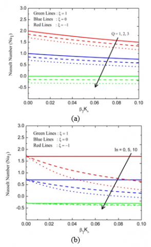
Figures 18$(a)$ and 19 (a) show the effect of $Q$ on the Nusselt number. It is observed that the heat transfer rate increases with the increase in the value of $Q$ at the wall $y=0$ while the reverse trend occurs at the microchannel wall $y=1$ . In addition, it is found that the heat transfer rate is higher in the case of asymmetric heating than that of the symmetric heating. Figures 18 (b) and 19 (b) depict the effect of the fluid-wall interaction parameter on the Nusselt number. It is seen that the heat transfer rate decreases by rising the values of $\ln , \beta_{v} K_{n} \& \xi$ .
Figure 15. Volume flow rate $Q_{m}$ for different values of $Q$ and $\alpha$
Figure 16. Skin friction $\tau_{0}$ for different values of $Q$ and $\alpha$
Figure 17. Skin friction $\tau_{1}$ for different values of $Q$ and $\alpha$
Figure 18. Nusselt number $N u_{0}$ for different values of $Q$ and $\ln$
Figure 19. Nusselt number $N u_{1}$ for different values of $Q$ and $\ln$
Table 2. Numerical values of volume flow rate $\left(Q_{m}\right)$ for various values of $M, P m, \beta, n, l n$ when $Q=2$ and $\alpha=0.5$ along with
the slope of data points
|
M |
Pm |
$\boldsymbol{\beta}$ |
n |
ln |
Qm |
|
||||
|
$\xi=1$ |
$\xi=0$ |
|
||||||||
|
$\begin{aligned} & \boldsymbol{\beta}_{v} \boldsymbol{K}_{\boldsymbol{n}} \\=& \mathbf{0} \cdot \mathbf{0} 5 \end{aligned}$ |
$\boldsymbol{\beta}_{v} \boldsymbol{K}_{\boldsymbol{n}}$ |
$\begin{aligned} & \boldsymbol{\beta}_{v} \boldsymbol{K}_{\boldsymbol{n}} \\=& \mathbf{0} \cdot \mathbf{0} \mathbf{5} \end{aligned}$ |
$\boldsymbol{\beta}_{v} \boldsymbol{K}_{n}$ |
|||||||
|
1 |
0.5 |
0.5 |
2 |
1.667 |
0.0625 |
0.0802 |
0.0296 |
0.0387 |
||
|
1.5 |
0.5 |
0.5 |
2 |
1.667 |
0.0624 |
0.0801 |
0.0295 |
0.0387 |
||
|
2 |
0.5 |
0.5 |
2 |
1.667 |
0.0622 |
0.0799 |
0.0295 |
0.0386 |
||
|
Slope |
-0.0003 |
-0.0003 |
-0.0001 |
-0.0001 |
|
|||||
|
5 |
1 |
0.5 |
2 |
1.667 |
0.0568 |
0.0745 |
0.0272 |
0.0363 |
||
|
5 |
1.5 |
0.5 |
2 |
1.667 |
0.054 |
0.0716 |
0.026 |
0.0351 |
||
|
5 |
2 |
0.5 |
2 |
1.667 |
0.0511 |
0.0688 |
0.0247 |
0.0339 |
||
|
Slope |
-0.0057 |
-0.0057 |
-0.0025 |
-0.0024 |
||||||
|
5 |
0.5 |
1 |
2 |
1.667 |
0.0874 |
0.114 |
0.0417 |
0.0554 |
||
|
5 |
0.5 |
1.5 |
2 |
1.667 |
0.1034 |
0.1352 |
0.0494 |
0.0659 |
|
|
|
5 |
0.5 |
2 |
2 |
1.667 |
0.1137 |
0.1491 |
0.0544 |
0.0727 |
||
|
Slope |
0.0263 |
0.0351 |
0.0127 |
0.0173 |
||||||
|
5 |
0.5 |
0.5 |
1 |
1.667 |
0.1863 |
0.2106 |
0.3459 |
0.3265 |
||
|
5 |
0.5 |
0.5 |
1.5 |
1.667 |
0.0716 |
0.0899 |
0.0514 |
0.0587 |
||
|
5 |
0.5 |
0.5 |
2 |
1.667 |
0.0583 |
0.0761 |
0.0261 |
0.0356 |
||
|
Slope |
-0.128 |
-0.1345 |
-0.3198 |
-0.2909 |
||||||
|
5 |
0.5 |
0.5 |
2 |
1 |
0.0586 |
0.0747 |
0.0277 |
0.0357 |
||
|
5 |
0.5 |
0.5 |
2 |
1.5 |
0.0595 |
0.0767 |
0.0282 |
0.0371 |
||
|
5 |
0.5 |
0.5 |
2 |
2 |
0603 |
0.788 |
0.0288 |
0.0386 |
|
|
|
Slope |
0.0017 |
0.0041 |
0.0011 |
0.0029 |
||||||
Table 3. Numerical values of skin friction $\left(\tau_{0}\right)$ for various values of $M, P m, \beta, n, l n$ when $Q=2, \alpha=0.5$ along with the slope of data points
|
M |
Pm |
$\boldsymbol{\beta}$ |
n |
ln |
$\boldsymbol{\tau}_{0}$ |
|||||
|
$\xi=1$ |
$\xi=0$ |
|||||||||
|
$\boldsymbol{\beta}_{v} \boldsymbol{K}_{n}$ |
$\boldsymbol{\beta}_{v} \boldsymbol{K}_{n}$ |
$\boldsymbol{\beta}_{v} \boldsymbol{K}_{n}$ |
$\beta_{v} K_{n}$ |
|||||||
|
1 |
0.5 |
0.5 |
2 |
1.667 |
0.288 |
0.3013 |
0.1035 |
0.1185 |
||
|
1.5 |
0.5 |
0.5 |
2 |
1.667 |
0.288 |
0.3013 |
0.1036 |
0.1187 |
||
|
2 |
0.5 |
0.5 |
2 |
1.667 |
0.288 |
0.3013 |
0.1038 |
0.1189 |
||
|
Slope |
0 |
0 |
0.0003 |
0.0004 |
||||||
|
5 |
1 |
0.5 |
2 |
1.667 |
0.288 |
0.3013 |
0.1099 |
0.125 |
||
|
5 |
1.5 |
0.5 |
2 |
1.667 |
0.288 |
0.3013 |
0.1132 |
0.1283 |
||
|
5 |
2 |
0.5 |
2 |
1.667 |
0.288 |
0.3013 |
0.1164 |
0.1316 |
||
|
Slope |
0 |
0 |
0.0065 |
0.0066 |
||||||
|
5 |
0.5 |
1 |
2 |
1.667 |
0.4319 |
0.4519 |
0.1624 |
0.185 |
||
|
5 |
0.5 |
1.5 |
2 |
1.667 |
0.5183 |
0.5423 |
0.1966 |
0.2238 |
||
|
5 |
0.5 |
2 |
2 |
1.667 |
0.5759 |
0.6025 |
0.2198 |
0.25 |
||
|
Slope |
0.144 |
0.1506 |
0.0574 |
0.065 |
||||||
|
5 |
0.5 |
0.5 |
1 |
1.667 |
-0.2481 |
-0.2303 |
-0.4344 |
-0.4163 |
||
|
5 |
0.5 |
0.5 |
1.5 |
1.667 |
0.291 |
0.3068 |
0.1075 |
0.1244 |
||
|
5 |
0.5 |
0.5 |
2 |
1.667 |
0.3064 |
0.3198 |
0.1251 |
0.1402 |
||
|
Slope |
0.5545 |
0.5501 |
0.5595 |
0.5565 |
||||||
|
5 |
0.5 |
0.5 |
2 |
1 |
0.2825 |
0.2905 |
0.1016 |
0.1122 |
||
|
5 |
0.5 |
0.5 |
2 |
1.5 |
0.2866 |
0.2985 |
0.1054 |
0.1193 |
||
|
5 |
0.5 |
0.5 |
2 |
2 |
0.2907 |
0.3067 |
0.1091 |
0.1264 |
||
|
Slope |
0.0082 |
0.0162 |
0.0075 |
0.0142 |
||||||
Table 4. Numerical values of skin friction $\left(\tau_{1}\right)$ for various values of $M, P m, \beta, n, l n$ when $Q=2, \alpha=0.5$ along with the slope of
|
M |
Pm |
$\boldsymbol{\beta}$ |
n |
ln |
$\tau_{1}$ |
|||
|
$\xi=1$ |
$\xi=\mathbf{0}$ |
|||||||
|
$\begin{aligned} & \boldsymbol{\beta}_{v} \boldsymbol{K}_{\boldsymbol{n}} \\=& \mathbf{0} \cdot \mathbf{0} 5 \end{aligned}$ |
$\beta_{v} K_{n}$ |
$\beta_{v} K_{n}$ |
$\boldsymbol{\beta}_{v} \boldsymbol{K}_{\boldsymbol{n}}$ |
|||||
|
1 |
0.5 |
0.5 |
2 |
1.667 |
-0.2831 |
-0.2954 |
-0.1678 |
-0.1697 |
|
1.5 |
0.5 |
0.5 |
2 |
1.667 |
-0.2831 |
-0.2954 |
-0.1677 |
-0.1696 |
|
2 |
0.5 |
0.5 |
2 |
1.667 |
-0.2831 |
-0.2954 |
-0.1674 |
-0.1693 |
|
Slope |
0 |
0 |
0.0004 |
0.0004 |
||||
|
5 |
1 |
0.5 |
2 |
1.667 |
-0.2831 |
-0.2954 |
-0.1614 |
-0.1632 |
|
5 |
1.5 |
0.5 |
2 |
1.667 |
-0.2831 |
-0.2954 |
-0.1581 |
-0.1599 |
|
5 |
2 |
0.5 |
2 |
1.667 |
-0.2831 |
-0.2954 |
-0.1548 |
-0.1566 |
|
Slope |
0 |
0 |
0.0066 |
.0066 |
||||
|
5 |
0.5 |
1 |
2 |
1.667 |
-0.4247 |
-0.443 |
-0.2445 |
-0.2473 |
|
5 |
0.5 |
1.5 |
2 |
1.667 |
-0.5097 |
-0.5316 |
-0.2917 |
-0.295 |
|
5 |
0.5 |
2 |
2 |
1.667 |
-0.5663 |
-0.5907 |
-0.3228 |
-0.3265 |
|
Slope |
-0.146 |
-0.147 |
-0.073 |
-0.072 |
||||
|
5 |
0.5 |
0.5 |
1 |
1.667 |
-0.3024 |
-0.3212 |
-0.1804 |
-0.1875 |
|
5 |
0.5 |
0.5 |
1.5 |
1.667 |
-0.2913 |
-0.3063 |
-0.1754 |
-0.1754 |
|
5 |
0.5 |
0.5 |
2 |
1.667 |
-0.2831 |
-0.2954 |
-0.1647 |
-0.1665 |
|
Slope |
0.0193 |
0.0258 |
0.0157 |
0.021 |
||||
|
5 |
0.5 |
0.5 |
2 |
1 |
-0.2785 |
-0.2857 |
-0.1634 |
-0.1623 |
|
5 |
0.5 |
0.5 |
2 |
1.5 |
-0.282 |
-0.2929 |
-0.1643 |
-0.1654 |
|
5 |
0.5 |
0.5 |
2 |
2 |
-0.2855 |
-0.3002 |
-0.1655 |
-0.169 |
|
Slope |
-0.007 |
-0.0145 |
-0.0021 |
-0.0067 |
||||
The numerical values of $Q_{m}$ for various values of $M, P m, \beta, n$ and $l n$ when $Q=2$ and $\alpha=0.5$ are recorded for the cases of $\xi=1$ and $\xi=0$ in table 2 . Also, the slope of linear regression using data points in estimated to know the amount of increase or decrease in the $Q_{m}$ . It is also seen that, the $Q_{m}$ is a declining function of $M, P m$ and $n$ whereas $Q_{m}$ is an increasing function of $\beta$ and $l n$ . Impact of $\beta$ on $Q_{m}$ is more significant than that of $l n$ . Tables 3 and 4 present the numerical values of skin friction coefficient at $y=0$ and $y=$ 1 respectively for various values of $M, P m, \beta, n$ and $l n$ when $Q=2$ and $\alpha=0.5 .$ It is found that, the $\tau_{0}$ is an increasing function of $M, P m, \beta, n$ and $l n .$ Impact of $n$ on $\tau_{0}$ is more significant than that of $M, P m, \beta,$ and $l n .$ From tables 4 it is noticed that $\tau_{1}$ is an increasing function of $M, P m$ and $n$ whereas it is a declining function of $\beta$ and $l n .$
7.1 Correlation coefficient and probable error
The correlation coefficient $(r)$ and probable error $(P E)$ are calculated for skin friction co-efficient and Nusselt number for various parameters. The nature of the relationship for variables considered was determined by the sign of $r$ . The significance precision of the correlation coefficient is calculated by using probable error $(P E) .$ If $r>6 \cdot P E$ then the correlation is said to be significant according to Fisher $[22]$ . The probable error is given by:
$P E=\left(\frac{1-r^{2}}{\sqrt{j}}\right) 0.6745$
where j denotes the number of observations.
Table 5. Correlation coefficient $(\mathrm{r}),$ Probable error $(\mathrm{PE})$ and $\left|\frac{r}{p E}\right|$values for $\tau_{0}$ with respect to the parameters $Q, \beta, \alpha, n, l n$ and $\beta_{v} K_{n}$
|
$\boldsymbol{\tau}_{\mathbf{0}}$ |
|||
|
Parameter |
r |
PE |
$|\boldsymbol{r} / \boldsymbol{P} \boldsymbol{E}|$ |
|
Q |
0.998274 |
0.001163182 |
858.2266 |
|
$\beta$ |
0.999952 |
3.23752E-05 |
30886.34 |
|
$\alpha$ |
0.999964 |
2.42816E-05 |
41182.03 |
|
n |
-0.99838 |
0.001091132 |
914.996 |
|
ln |
0.989949 |
0.00674533 |
146.7607 |
|
$\beta_{v} K_{n}$ |
-0.99997 |
2.09092E-05 |
47824.41 |
|
$\boldsymbol{\tau}_{\mathbf{1}}$ |
|||
|
Parameter |
r |
PE |
$|\boldsymbol{r} / \boldsymbol{P} \boldsymbol{E}|$ |
|
Q |
-0.99827 |
0.001163182 |
858.2266 |
|
$\beta$ |
-0.99995 |
3.23752E-05 |
30886.34 |
|
$\alpha$ |
-0.99996 |
2.42816E-05 |
41182.03 |
|
n |
0.984315 |
0.010496563 |
93.77499 |
|
ln |
-0.98995 |
0.00674533 |
146.7607 |
|
$\beta_{\nu} K_{n}$ |
-0.99997 |
1.88857E-05 |
52948.53 |
|
$\boldsymbol{N} \boldsymbol{u}_{\mathbf{0}}$ |
|||
|
Parameter |
r |
PE |
$|\boldsymbol{r} / \boldsymbol{P} \boldsymbol{E}|$ |
|
Q |
0.999989 |
7.41946E-06 |
134779.2 |
|
n |
-0.99998 |
1.61878E-05 |
61773.41 |
|
ln |
-0.94388 |
0.036790787 |
25.65534 |
|
$\beta_{v} K_{n}$ |
-0.99976 |
0.000165232 |
6050.604 |
Table 8. Correlation coefficient $(\mathrm{r}),$ Probable error $(\mathrm{PE})$ and $\left|\frac{r}{P E}\right|$ values $N u_{1}$ for with respect to the parameters $Q, n, l n$ and $\beta_{v} K_{n}$
|
$N u_{1}$ |
|||
|
Parameter |
r |
PE |
$|\boldsymbol{r} / \boldsymbol{P} \boldsymbol{E}|$ |
|
Q |
-0.99999 |
1.01174E-05 |
98837.9 |
|
n |
0.928734 |
0.046356077 |
20.03478 |
|
ln |
-0.94868 |
0.033725191 |
28.1298 |
|
$\beta_{\nu} K_{n}$ |
-0.99965 |
0.000233337 |
4284.171 |
7.2 Regression analysis
The regression analysis is made to estimate the skin friction co-efficient and Nusselt number by multivariable linear regression models. Since the curves of τ and Nu (see Figures 16-19) are linear in nature the linear regression model is chosen specifically to estimate the same. The estimated models are given below:
$\tau_{0 e s t}=b_{Q} Q+b_{M} M+b_{P m} P m+b_{\beta} \beta+b_{\alpha} \alpha+b_{n} n+b_{l n} l n$
$+b_{\beta_{\nu K n}} \beta_{\nu} K n+C_{1}$
$\tau_{1 e s t}=b_{Q} Q+b_{M} M+b_{P m} P m+b_{\beta} \beta+b_{\alpha} \alpha+b_{n} n+b_{l n} l n$
$+b_{\beta_{\nu K n}} \beta_{\nu} K n+C_{2}$
$N u_{0 e s t}=b_{Q} Q+b_{n} n+b_{l n} \ln +b_{\beta_{\nu} K n} \beta_{\nu} K n+C_{3}$
$N u_{1 e s t}=b_{Q} Q+b_{n} n+b_{l n} l n+b_{\beta_{\nu} K n} \beta_{\nu} K n+C_{4}$
where, $b_{Q}, b_{M}, b_{P m}, b_{\beta}, b_{\alpha}, b_{n}, b_{l n}$ and $b_{\beta_{v} K_{n}}$ are the estimated regression coefficient and $C_{1}, C_{2}, C_{3}$ and $C_{4}$ are constants. The $\tau_{0}$ values are estimated from 30 set of random values of $Q, M, \beta, \alpha, n,$ ln $\& \beta_{v} K_{n} \in[0.1,0.6]$ and $P m \in[0.01,0.07]$ for regression model. It is found that all the physical parameters achieve significance value<0.05 for significant regression coefficients except for the parameters $Q$ and $P m$ (see Table 9).
Table 9. Regression coefficients for the multiple linear regression model for $\tau_{0}$
|
Model |
Unstandardized Coefficients |
Significance |
|
|
b |
Standard Error |
|
|
|
(Constant) |
-.111 |
.007 |
.000 |
|
Q |
.029 |
.001 |
.000 |
|
M |
-.001 |
.001 |
.459 |
|
Pm |
-.003 |
.004 |
.438 |
|
β |
.440 |
.007 |
.000 |
|
α |
.264 |
.007 |
.000 |
|
n |
-.022 |
.005 |
.000 |
|
ln |
.011 |
.001 |
.000 |
|
βvKn |
.456 |
.005 |
.000 |
The estimated $\tau_{0}$ is given by:
$\tau_{0 e s t}=0.029 Q-0.001 M-0.003 P m+0.440 \beta$
$+0.264 \alpha-0.022 n$
$+0.011 l n+0.456 \beta_{v} K n-0.111$
The above equation implies that the parameters $Q, \beta, \alpha, l n, \beta_{v} K_{n}$ and $M, P m, n$ have a positive and negative impact on $\tau_{0}$ correspondingly. Similarly, $\tau_{1}$ values are estimated from 30 set of random values of $Q, M, \beta, \alpha, n, l n, \beta_{v} K_{n} \& P m \in[0.1,0.4]$ for the regression model. It is evident from table 10 that, all the physical parameters have the significance value<0.05 for significant regression coefficients except for the parameters $Q$ and $P m .$
Table 10. Regression coefficients for the multiple linear regression model for $\tau_{1}$
|
Model |
Unstandardized Coefficients |
Significance |
|
|
b |
Standard Error |
|
|
|
(Constant) |
0.125 |
0.009 |
0.000 |
|
Q |
-0.031 |
0.001 |
0.000 |
|
M |
-0.001 |
0.001 |
.520 |
|
Pm |
-0.005 |
0.008 |
.544 |
|
β |
-0.452 |
0.008 |
.000 |
|
α |
-0.256 |
0.015 |
.000 |
|
n |
0.035 |
0.008 |
.000 |
|
ln |
-0.013 |
0.002 |
.000 |
|
βvKn |
-0.434 |
0.009 |
.000 |
The estimated regression model of $\tau_{1}$ is given by:
$\begin{array}{rl}{\boldsymbol{\tau}_{1 e s t}=-\mathbf{0} \cdot \mathbf{0} 3} & {\mathbf{1} \boldsymbol{Q}-\mathbf{0} \cdot \mathbf{0} \mathbf{0} \mathbf{1} \boldsymbol{M}-\mathbf{0} \cdot \mathbf{0} \mathbf{0} 5 \boldsymbol{P} \boldsymbol{m}-\mathbf{0} \cdot \mathbf{4} 52 \boldsymbol{\beta}} \\ {-\mathbf{0} \cdot \mathbf{2} 56 \alpha+\mathbf{0} \cdot \mathbf{0} 35 \mathbf{n}} \\ {-\mathbf{0} \cdot \mathbf{0} \mathbf{1} \mathbf{3} \boldsymbol{l} \boldsymbol{n}-\mathbf{0} \cdot \mathbf{4} \mathbf{3} \mathbf{4} \boldsymbol{\beta}_{v} \boldsymbol{K} \boldsymbol{n}+\mathbf{0} \cdot \mathbf{1} \mathbf{2} \mathbf{5}}\end{array}$
The $\quad$ above $\quad$ equation $\quad$ depicts $\quad$ that $Q, M, P m, \beta, \alpha, l n, \beta_{v} K_{n}$ and $n$ have a negative and positive impact on $\tau_{1}$ respectively.
The $N u_{0}$ values are estimated from 30 set of random values of $Q, n, \ln \& \beta_{v} K_{n} \in[0.01,0.08]$ for regression model. It is found that all the physical parameters achieve the significance value $<0.05$ for significant regression coefficients (see Table 11).
Table 11. Regression coefficients for the multiple linear regression model for $N u_{0}$
|
Model |
Unstandardized Coefficients |
Significance |
|
|
b |
Standard Error |
||
|
(Constant) |
.170 |
.001 |
.000 |
|
Q |
.422 |
.000 |
.000 |
|
n |
-.309 |
.001 |
.000 |
|
ln |
-.006 |
.000 |
.000 |
|
βvkn |
-.153 |
.008 |
.000 |
The estimated regression model for $N u_{0}$ is given by:
$\begin{array}{rl}{N u_{0 e s t}=0.422 Q-0.309 n-0.006} & {l n-0.153 \beta_{v} K n} \\ {+0.170}\end{array}$
The above equation implies that the parameters $Q, n, \ln \& \beta_{v} K_{n}$ have a negative impact on $N u_{0} .$ Similarly, $N u_{1}$ values are estimated from 30 set of random values of $Q, n, \ln \& \beta_{v} K_{n} \in[0.1,0.8]$ for the regression model. It is evident from table 12 that, all the physical parameters have the significance value<0.05 for significant regression coefficients.
Table 12. Regression coefficients for the multiple linear regression model for $N u_{1}$
|
Model |
Unstandardized Coefficients |
Significance |
|
|
b |
Standard Error |
||
|
(Constant) |
-7.913 |
1.790 |
.000 |
|
Q |
-1.300 |
.451 |
.007 |
|
n |
20.486 |
2.350 |
.000 |
|
ln |
-1.355 |
.639 |
.041 |
|
$\beta_{\nu} K_{n}$ |
1.824 |
.834 |
.035 |
The estimated regression model for $N u_{1}$ is given by:
$\begin{array}{rl}{N u_{1 e s t}=-1.300 Q+20.486 n-1.355} & {l n+1.824 \beta_{v} K n} \\ {-7.913}\end{array}$
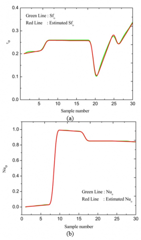
The above equation depicts that the parameters $Q \&$ ln have a negative impact on $N u_{1}$ whereas $n \& \beta_{v} K_{n}$ have a positive impact on $N u_{1} .$ The outcomes of estimated $\tau$ $\text { and } N u \text { are matching with actual } \tau \text { and } N u \text { (see Figure } 20)$.
Figure 20. Comparison of actual and estimated values of
$\tau_{0}$ and $N u_{0}$The role of the exponential heat source and quadratic convection in the flow of Casson fluid with an induced magnetic field under velocity slip and temperature jump is investigated analytically by using HPM. The following conclusions are drawn.
The solution obtained for and from the calculation and the regression equations are superimposed.
The authors (B Mahanthesh and Thriveni K) expresses thier sincere thanks to the Management, CHRIST (Deemed to be University), Bangalore, India for the support to complete this work.
|
b |
Distance between the plate (m) |
|
Cp |
Specific heat at constant pressure (J/kg K ) |
|
g |
Acceleration due to gravity (m/s2) |
|
$H _ { 0 } ^ { \prime }$ |
Applied magnetic field (T) |
|
$H _ { x } ^ { \prime }$ |
Dimensional induced magnetic field (A/m)
|
|
H |
Dimensionless induced magnetic field |
|
ln |
The fluid-wall interaction parameter |
|
J |
Induced current density (A/m2) |
|
M |
Induced magnetic parameter |
|
Pm |
Magnetic Prandtl number |
|
Pr |
Prandtl number |
|
Qm |
Dimensionless volume flow rate |
|
T’ |
The temperature of the fluid (K) |
|
T0 |
Reference temperature (K) |
|
u |
The dimensionless velocity of the fluid |
|
u’ |
The dimensional velocity of the fluid (m/s) |
|
Q |
Exponential heat source parameter |
|
n |
Exponential index |
|
k |
Thermal conductivity (W/m K) |
|
Greek symbols |
|
|
a |
Nonlinear convection parameter |
|
b |
Casson fluid parameter |
|
$\beta _ { 0 } , \beta _ { 1 }$ |
Coefficient of thermal expansion |
|
$\beta _ { t } , \beta _ { v }$ |
Dimensionless variables |
|
$\gamma$ |
The ratio of specific heat |
|
$\theta$ |
Dimensionless temperature |
|
$\rho$ |
Density (kg/m3) |
|
$\mu _ { e }$ |
Magnetic permeability (H/m) |
|
$v$ |
Kinematic viscosity (m2/s) |
|
$\sigma$ |
The electrical conductivity of the fluid (S/m) |
|
$\lambda$ |
Molecular mean free path |
|
$\sigma _ { t } , \sigma _ { v }$ |
Thermal and tangential momentum coefficient, respectively |
[1] Tuckerman, D.B., Pease, R.F.W. (1981). High-performance heat sinking for VLSI. IEEE Electron Device Letters, 2(5): 126-129. https://doi.org/10.1109/EDL.1981.25367
[2] Swift, G., Migliori, A., Wheatley, J. (1985). Construction of and measurements with an extremely compact cross-flow heat exchanger. Heat transfer Engineering, 6(2): 39-47. https://doi.org/10.1080/01457638508939623
[3] Weng, H.C. (2005). Natural convection in a vertical microchannel. Journal of Heat Transfer, 127(9): 1053-1056. https://doi.org/10.1115/1.1999651
[4] Jha, B.K., Aina, B., Joseph, S.B. (2014). Natural convection flow in a vertical microchannel with suction/injection. Proceedings of the Institution of Mechanical Engineers, Part E: Journal of Process Mechanical Engineering, 228(3): 171-180. https://doi.org/10.1177/0954408913492719
[5] Wang, C.Y., Ng, C.O. (2014). Natural convection in a vertical slit microchannel with superhydrophobic slip and temperature jump. Journal of Heat Transfer, 136(3): 034502. https://doi.org/10.1115/1.4025822
[6] Vajravelu, K., Cannon, J.R., Leto, J., Semmoum, R., Nathan, S., Draper, M., Hammock, D. (2003). Nonlinear convection at a porous flat plate with application to heat transfer from a dike. Journal of Mathematical Analysis and Applications, 277(2): 609-623. https://doi.org/10.1016/S0022-247X(02)00634-0
[7] Mahanthesh, B., Gireesha, B.J., Thammanna, G.T., Shehzad, S.A., Abbasi, F.M., Gorla, R.S.R. (2018). Nonlinear convection in nano Maxwell fluid with nonlinear thermal radiation: A three-dimensional study. Alexandria Engineering Journal, 57(3): 1927-1935. https://doi.org/10.1016/j.aej.2017.03.037
[8] Hayat, T., Qayyum, S., Alsaedi, A., Ahmad, B. (2018). Modern aspects of nonlinear convection and magnetic field in flow of thixotropic nanofluid over a nonlinear stretching sheet with variable thickness. Physica B: Condensed Matter, 537: 267-276. https://doi.org/10.1016/j.physb.2018.02.005
[9] Waqas, M., Khan, M.I., Hayat, T., Alsaedi, A. (2018). Effect of nonlinear convection on stratified flow of third grade fluid with revised Fourier-Fick relations. Communications in Theoretical Physics, 70(1): 025. https://doi.org/10.1088/0253-6102/70/1/25
[10] Gireesha, B.J., Kumar, P.S., Mahanthesh, B., Shehzad, S.A., Abbasi, F.M. (2018). Nonlinear gravitational and radiation aspects in nanoliquid with exponential space dependent heat source and variable viscosity. Microgravity Science and Technology, 30(3): 257-264. https://doi.org/10.1007/s12217-018-9594-9
[11] Tamoor, M., Waqas, M., Khan, M.I., Alsaedi, A., Hayat, T. (2017). Magnetohydrodynamic flow of Casson fluid over a stretching cylinder. Results in Physics, 7: 498-502. https://doi.org/10.1016/j.rinp.2017.01.005
[12] Pushpalatha, K., Reddy, J.R., Sugunamma, V., Sandeep, N. (2017). Numerical study of chemically reacting unsteady Casson fluid flow past a stretching surface with cross diffusion and thermal radiation. Open Engineering, 7(1): 69-76. https://doi.org/10.1515/eng-2017-0013
[13] Shashikumar, N.S., Prasannakumara, B.C., Gireesha, B.J., Makinde, O.D. (2018). Thermodynamics analysis of MHD casson fluid slip flow in a porous microchannel with thermal radiation. In Diffusion Foundations, 16: 120-139. https://doi.org/10.4028/www.scientific.net/DF.16.120
[14] Makinde, O.D., Eegunjobi, A.S. (2016). Entropy analysis of thermally radiating magnetohydrodynamic slip flow of Casson fluid in a microchannel filled with saturated porous media. Journal of Porous Media, 19(9). https://doi.org/10.1615/JPorMedia.v19.i9.40
[15] Eegunjobi, A.S., Makinde, O.D. (2017). MHD mixed convection slip flow of radiating Casson fluid with entropy generation in a channel filled with porous media. In Defect and Diffusion Forum, 374: 47-66. https://doi.org/10.4028/www.scientific.net/DDF.374.47
[16] Jha, B.K., Aina, B. (2016). Role of induced magnetic field on MHD natural convection flow in vertical microchannel formed by two electrically non-conducting infinite vertical parallel plates. Alexandria Engineering Journal, 55(3): 2087-2097. https://doi.org/10.1016/j.aej.2016.06.030
[17] Sivakumar, R., Vimala, S., Sekhar, T.V.S. (2015). Influence of induced magnetic field on thermal MHD flow. Num. Heat Trans., Part A: Applications, 68(7): 797-811. https://doi.org/10.1080/10407782.2014.994438
[18] Jha, B.K., Aina, B. (2017). Effect of induced magnetic field on MHD mixed convection flow in vertical microchannel. International Journal of Applied Mechanics and Engineering, 22(3): 567-582. https://doi.org/10.1515/ijame-2017-0036
[19] He, J.H. (1999). Homotopy perturbation technique. Computer Methods in Applied Mechanics and Engineering, 178(3): 257-262. https://doi.org/10.1016/S0045-7825(99)00018-3
[20] Biazar, J., Aminikhah, H. (2009). Study of convergence of homotopy perturbation method for systems of partial differential equations. Computers & Mathematics with Applications, 58(11): 2221-2230. https://doi.org/10.1016/j.camwa.2009.03.030
[21] Kumar, A., Singh, A.K. (2013). Unsteady MHD free convective flow past a semi-infinite vertical wall with induced magnetic field. Applied Mathematics and Computation, 222: 462-471. https://doi.org/10.1016/j.amc.2013.07.044
[22] Fisher, R.A. (1921). On the probable error of a coefficient of correlation deduced from a small sample. Metron, 1: 3-32.