Jasem M. Alhumoud* | Nourah Almashan
OPEN ACCESS
Muskingum method has been continuously receiving attention from the researchers for several reasons. It is a simple method, which can be used for flood routing without much complication as far as the procedural details are concerned. In addition, its parameters can be calculated using the record of past historical floods. It does not require a knowledge of the river bed geometry as the phenomenon can be reproduced well enough on the basis of the calibration carried out using experimental data relative to the extreme sections of most significantly long reaches. In this study, we have studied the applicability of linear and nonlinear Muskingum models on linear and nonlinear flood data. For the linear model three different methods were used to compare the accuracy of the actual and estimated outflow. The methods are: trial and error, least square, and direct optimization method. Subsequently, we have routed the flows based on the estimated parameters to compare the performance of these models. The results suggest a very good fit.
Muskingum models, linear, nonlinear, trial and error method, least square method, direct optimization method
Flood routing techniques are used for flood forecasting, reservoir design, watershed simulation, and comprehensive water resources projects. One category of flood routing is called the hydrology routing. The most well-known hydrology routing procedure is referred to as the Muskingum Method. McCarthy [1] first developed Muskingum flood routing for flood-control studies in the Muskingum River in Ohio, USA. Muskingum method has been continuously receiving attention from the researchers for several reasons. Firstly, it is a simple method, which can be used for flood routing without much complication as far as the procedural details are concerned. Its parameters can be calculated using the record of past historical floods. It does not require a knowledge of the river bed geometry as the phenomenon can be reproduced well enough on the basis of the calibration carried out using experimental data relative to the extreme sections of most significantly long reaches. Linear Muskingum models are (1) for continuity, and (2) for storage.
$\frac{d S}{d t}=I-Q$ (1)
$S_{t}=K\left[x I_{t}+(I-x) Q_{t}\right]$ (2)
The variables St, It, and Qt are simultaneous storage, inflow, and outflow, respectively, during the passage of a flood through the reach at time t; x and K are constants. Physically speaking, K is considered to represent the average reach travel time and will be equal to the time difference between the centroids of inflow and outflow hydrographs. The coefficient x is used to weigh the relative effects of inflow and outflow on reach storage and can take values from 0 to 0.5.
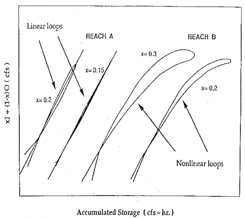
Traditionally, the parameters are estimated by plotting accumulated storage versus weighted flow of a given reach (Figure 1). Although some reaches may exhibit nonlinear loops, the value of x that gives a nearly collapsed loop, approximating a straight line as determined by visual judgment is considered the best value. The coefficient K is then the reciprocal of the slope of the straight line best representing the loop.
The trial and error graphical approach, which have been used for decades, is time consuming and prone to subjective interpretation. Furthermore, the visual judgement may not correctly identify the best among several nearly collapsed loops when all may appear acceptable.
Figure 1. Typical linear and nonlinear storage-weighted flow relationship
In case where the storage versus weighted flow relationship is not linear as implied in the original Muskingum model, using a linear form of Muskingum model may introduce considerable error. If the relationship for a reach is discovered to be nonlinear, as seen in Figure 1, the nonlinear models given by Eqns. (3) and (4) may be more appropriate [2-6].
$\mathrm{S}_{\mathrm{t}}=\mathrm{K}\left[\mathrm{x} \mathrm{I}_{\mathrm{t}}-(\mathrm{I}-\mathrm{x}) \mathrm{Q}_{\mathrm{t}}\right]^{\mathrm{n}}$ (3)
$\mathrm{S}_{\mathrm{t}}=\mathrm{K}\left[\mathrm{x} I_{t}^{n}-(\mathrm{I}-\mathrm{x}) Q_{t}^{n}\right]$ (4)
These models have an additional parameter n, which cannot be determined graphically from recorded inflow and outflow hydrographs, and alternative parameter estimation methods must be used.
In this study, we have studied the applicability of linear and nonlinear models on linear and nonlinear flood data. Subsequently, we have routed the flows based on the estimated parameters to compare the performance of these models.
The Muskingum method consists in a spatially lumped form of continuity equation and a linear storage discharge relationship for a specified river reach. These equations can be rewritten as:
$\frac{d S}{d t}=I-Q$ (5)
S = K [x I + (1 - x) Q] (6)
Combining Eqns. (5) and (6)
$Q+K(I-x) \frac{d Q}{d t}=I-K x \frac{d I}{d t}$ (7)
In order to solve Eq. (7) uniquely, an initial condition must be specified. From a hydrologic standpoint, this initial condition must reflect physical realism. A survey of literature indicates that this has been specified in three ways:
I(O) = Q(O) = 0 (8)
I(O) = Q(O) = 10 (9)
1(O) = Q (T), T ˃ 0 (10)
where T is time taken by the flood wave to reach the downstream end of the river reach.
If Eq. (7) is solved using Eq. (8) as the initial condition, the solution is then:
$Q(t)=\int_{0}^{t} h(t-y) I(y) d y$ (11)
where h(t) is the instantaneous unit hydrograph (IUH) of the river reach and can be expressed as:
$h(t)=\frac{I}{K(I-x)^{2}} e^{-\frac{t}{[K(I-x)]}}-\frac{x}{I-X} \delta(t)$ (12)
where δ(t) is the Dirac δ - function or impulse inflow.
However, if Eq. (7) is solved using Eq. (9) as the initial condition, the solution is then:
$Q(t)=\frac{I_{0}}{(I-x)} e^{-\frac{t}{[K(I-x)]}}-\frac{x}{I-x} I(t)+\frac{I}{K(I-x)^{2}} \int_{0}^{t} e^{-\frac{t-S}{[K(I-x)]}} I(s) d s$ (13)
The initial condition given by Eq. (10) was proposed by Gill [7-8]. If Eq. (7) is solved using this condition then, for T ≤ t the solution would be:
$Q(t)=-\frac{x}{(I-x)} I(t)+\left[Q(T)+\frac{x}{(I-x)} I(T)\right] e^{-\frac{t-S}{[K(I-x)]}}+\frac{I}{K(I-x)} \int_{T}^{t} e^{-\frac{t-S}{[K(I-x)]}} I(s) D s$ (14)
This solution was obtained by Singh and McCann [9-10] with an explicit statement of the initial condition assumed.
A careful consideration of Eq. (14) shows that the inflow I on the interval 0 < t < T does not affect the outflow at times t > T.
It seems more appropriate that any lag time T to be imposed on Muskingum method should be imposed through the basic equations, not through the initial condition. Using the Muskingum assumption of a unique stage-discharge relationship m St. Venant equations, Cunge [8, 11] derived a partial differential equation for the Muskingum method. He then showed that the Muskingum method did not allow for wave damping, and that wave attenuation was due to errors arising from numerical approximation of the Muskingum equation. This, of course, is valid if it is assumed that the lumped system can be transformed into a distributed system, the Muskingum method has a dynamic basis and that this basis lies in St. Venant equations. It can be seen that this assumption is no more valid than the Muskingum hypothesis itself and has no particular basis other than to try to predicate a physical basis for a purely empirical assumption.
The Muskingum method is not a translatory solution. Further, it can be shown that there is no unique dynamical analogy of the Muskingum method even if the assumption of its dynamic basis is made.
Through an entirely different approach, translatory solutions for the Muskingum method have been obtained for particular parameter values and some assumptions on inflow [8, 12, 13]. If Eq. (7) is written in a finite difference form (using forward difference formula) then:
Qn = C0 I0 + C1 In-1 + C2 Qn-1 (15)
where:
$C_{0}=\frac{(-K x+0.5 \Delta t)}{C_{3}}$; $C_{1}=\frac{(K x+0.5 \Delta t)}{C_{3}}$; $C_{2}=\frac{(K-K x+0.5 \Delta t)}{C_{3}}$ and $C_{3}=(K-K x-0.5 \Delta t)$ (16)
Here Δt is the routing period, and C0 + C1 + C2 = 1. The approximate translator solution is possible only if l and Q can be approximated linearly over M. This implies that Δt should be very small so that this assumption is not violated.
Consequently, K will be very small and the channel reach under consideration will have to be short enough to have such a small approximation travel time. However, if we consider a continuous solution given by Eq. (13), then it is immediately clear that regardless of the choice of K and x, this solution is not translatory. To illustrate, consider:
$I(t)=\left[\begin{array}{ll}{I(0)+\sin t,} & {0 \leq t<\pi} \\ {I(0)} & {, \quad t \geq \pi}\end{array}\right]$ (17)
$Q(t)=\frac{I_{0}}{I-x} e^{-\frac{-t}{[K(I-x)]}}-\frac{x}{(I-x)} I(t)+\frac{K e^{-\frac{t}{[K(I-x)]}}}{K^{2}(I-x)^{2}+I}\left(1+e^{-\frac{\pi}{[K(I-x)]}}\right)+\frac{I_{0}}{(I-x)}\left(1+e^{-\frac{t}{[K(I-x)]}}\right), t \geq \pi$ (18)
Evidently Q (t + T) ≠ I(t) for any T.
On the other hand, if we consider equation 11 then we may not obtain translator solutions for any choice of K and x. This can be seen to be true by considering the above example input in Eq. (17) with I0=0. The above discussion shows that the Muskingum method, as proposed by McCarthy [1], is not a translatory solution. This method is a black box type and is not based on hydraulic equations of open channel flow. It says nothing about the spatial variability of inflow, outflow and storage [14-17].
3.1 Trial and error method
In the conventional graphical method, weighted flow given by Eq. (18) is plotted against the accumulated storage given by Eq. (19) for several selected values of x. The value of x which gives the narrowest loop is accepted as the Muskingum x. The narrowest loop is then represented by a straight line, and the reciprocal of the slope of this line is taken as storage constant K.
$S_{2}=S_{1}+(\overline{I}-\overline{Q}) \Delta t$ (19)
where,
$\overline{I}=\frac{I_{n}+I_{n+1}}{2}, \overline{Q}=\frac{Q_{n}+Q_{n+1}}{2}$ Weighted flow $=\mathrm{x} \mathrm{I}_{\mathrm{nt} 1}+(1-\mathrm{x}) \mathrm{Q}_{\mathrm{nt} 1}$ (20)
Instead of drawing the accumulated storage against weighted flow for each trial value of x, and then choosing the best fit line by visual judgement, I developed a computer program to compute the sum of the squares of the deviations from the best fit line. For each particular value of x, pairs of values for accumulated storage and weighted flow were computed using the given inflow and outflow hydrographs ordinates. The best fit line through these points was then determined by the method of least squares with the condition that this line should pass through the initial point when I0 = Q0. For each value of x, and the corresponding straight line giving the best fit line between weighted discharge and accumulated storage, the error sum of squares was recorded, and the value of x resulting in the least error sum of squares will be chosen as the Muskingum parameter x. The storage constant K will be the reciprocal of the slope of the best fit line. This procedure is summarized below.
Let y = weighted discharge
b = slope of the straight line.
Then,
y = y0 + b (S – S0) (21)
And
$s u m=\sum\left[y-\left[y_{0}+b\left(S-S_{0}\right)\right]\right]^{2}=\sum\left[\mathrm{y}-\mathrm{y}_{0}-\mathrm{b} \mathrm{S}+\mathrm{b} \mathrm{S}_{0}\right.$ (22)
$\frac{d(s u m)}{d b}=0=\sum 2\left(y-y_{0}-b S+b S_{0}\right)\left(-S+S_{0}\right)-\sum y S+y_{0} \sum S+b \sum S^{2}-b S_{0} \sum S+S_{0} \sum y-n y_{0} S_{0}-$
$b S_{0} \sum S+n b S_{0}^{2}=0$ (23)
where n = number of data points except the initial point.
$b\left[\Sigma S^{2}-2 S_{0} \sum S+n S_{0}^{2}\right]=\sum y S-y_{0} \sum S-S_{0} \sum y+n y_{0} S_{0}$ (24)
$b=\frac{\sum y S-y_{0} \sum S-S_{0} \sum y+n y_{0} S_{0}}{\sum S^{2}-2 S_{0} \sum S+n S_{0}^{2}}$ (25)
If the initial storage is considered as zero,
sum = ⅀ (y – y0 – b S)2 (26)
$\frac{d(s u m)}{d b}=0=\sum 2\left(y-y_{0}-b S\right)(-S)$ (27)
⅀ y S – y0 ⅀S – b ⅀ S2 = 0 (28)
Then
$b=\frac{\sum y S-y_{0} \sum S}{\sum S^{2}}$ (29)
It should be noted that Eq. (29) is a special case of Eq. (25) for So= 0.
3.2 Least square method
This method is based on minimizing the sum of squares of deviations between observed storage and computed storage for a given inflow-outflow sequence. Mathematically:
$E=\sum_{j=1}^{N}\left[S_{0}(j)-S_{e}(j)\right]^{2} \rightarrow \min$ (30)
where S0 (j) is the observed storage for the jth time interval; Se (j) is the estimated storage for the jth time interval; and N is the number of observations. E is the error function to be minimized. Two cases are distinguished.
Case A: C ≠ 0 where C is the difference between absolute and relative storages. Eq. (21) can be written as (dropping j for brevity and assuming A = K x and B =K (1-x):
$\mathrm{E}=\sum_{j=1}^{N}\left[S_{0}-\mathrm{x} \mathrm{K} \mathrm{I}-\mathrm{K}(1-\mathrm{x}) \mathrm{Q}-\mathrm{C}\right]^{2}$ (31)
Thus we obtain:
$A=\frac{y_{1}}{y_{2}}-B\left(\frac{y_{3}}{y_{2}}\right)$, $B=\frac{y_{1} z_{2}-z_{1} y_{2}}{z_{2} y_{3}-y_{2} z_{1}}$ and $C=\frac{\sum S_{0}-A \sum I-B \sum Q}{N}$ (32)
where
$y_{1}=\sum S_{0} I-\frac{\left(\sum s_{0} \sum I\right)}{N}$, $y_{2}=\sum I^{2}-\frac{(\Sigma I)^{2}}{N}$ and $y_{3}=\frac{\sum Q I-\Sigma Q \Sigma I}{N}$ (33)
$z_{1}=\sum S_{0} Q-\frac{\left(\sum S_{0} \sum Q\right)}{N}$, $z_{2}=\sum I Q-\frac{(\Sigma I \Sigma Q)}{N}$ and $\Sigma Q^{2}-\frac{(\Sigma Q \Sigma Q)}{N}$ (34)
Therefore:
K = A+ B and X= A/(A+B) (35)
Thus K, x and C can be determined objectively and conveniently.
Case B: C = 0. Solving for A and B as before:
$A=\frac{\left(\sum s_{0} I \sum Q^{2}-\sum s_{0} Q \sum I Q\right)}{D}$, $B=\frac{\left(\sum s_{0} I \sum I^{2}-\sum S_{0} Q \sum I Q\right)}{D}$ and $D=\sum I^{2} \sum Q^{2}-\left(\sum I Q\right)^{2}$ (36)
And hence K and x can be determined from Eq. (34).
3.3 Direct Optimization (DO) method
The ditect optimization (DO) method determines directly the routing coefficients C0, C1, and C2 without estimating K and x. The method is based on minimizing the difference between observed outflow hydrograph and computed hydrograph. Therefore, this method is also a least-squares optimization method and is in principle, equivalent to the least squares method defined previously.
There are, in fact, only two unknowns since the third is known from C0 + C1 + C2 = 1. If we choose C1, and C2 to be the unknowns then:
$x=\frac{c_{1}+0.5 c_{2}-0.5}{c_{1}+c_{2}}$ (37)
$K=\frac{\Delta t\left(C_{1}+C_{2}\right)}{1-C_{2}}$ (38)
Further, rearranging
C1 (In – In-1) + C2 (In – Qn-1) = In - Qn (39)
If we define:
Rn = In – Qn; Fn = In – In-1; and Gn = In – Qn-1 (40)
Then
Rn = C1 Fn + C2 Gn (41)
The error function (dropping the subscript n for brevity) then follows:
$E=\Sigma_{1}^{N}\left(R_{0}-R_{e}\right)^{2} \rightarrow \min$ (42)
where subscripts 0 and e denote observed the estimated R values, respectively.
Following the usual procedure:
⅀R0 F = C1 ⅀F2 + C2 ⅀F G and ⅀R0 G = C1 ⅀F G + C2 ⅀G2 (43)
Solving for C1 and C2:
$C_{1}=\frac{\left(\sum R_{0} F \sum G^{2}-\Sigma R_{0} G \sum F G\right)}{D E T}$ and $C_{2}=\frac{\left(\sum R_{0} G \sum F^{2}-\sum R_{0} F \sum F G\right)}{D E T}$ (44)
where
$D E T=\Sigma G^{2} \Sigma F^{2}-(\Sigma F G)^{2}$ (45)
Thus, once C1 and C2 are determined, K and x can be obtained.
3.4 Nonlinear method
Through an analysis of stream flow records at the upstream and downstream ends of a river reach, it is possible to construct a set of data comprising the inflow rates at the upstream end of the reach, the outflow rates at downstream end of the reach and the storage volumes in the reach at selected times over some historical period. These data may be denoted by:
St = actual or measured storage in the reach at time t
It = actual or measured inflow rate at the top of the reach at time t
Qt = actual or measured outflow rate at the bottom of the reach at time t.
The standard, nonlinear Muskingum model for channel routing assumes a relationship between storage, inflow and outflow defined by Eq. (44). A standard selection procedure for parameters of the model is to minimize the sum of the squared deviations of model-predicted storage and actual storage. One way to define this procedure for the standard nonlinear model is with the mathematical model given by Eq. (47) and 48.
$S_{t}=K\left[x I_{t}^{n}+(1-x) Q_{t}^{n}\right]$ (46)
$N=\sum_{t}\left(S_{t}-P_{s t}\right)^{2}$ (47)
$P_{s t}=K\left[x I_{t}^{n}+(1-x) Q_{t}^{n}\right]$ (48)
where Pst =model - predicted storage value;
N = error sum of squares.
One of the solution method for the mathematical program is: 1- select a group of values for n (e.g. n = 0.05, 0.10, ...); for each value of n, solve the resulting mathematical model using traditional calculus methods by setting all partial derivatives equal to zero and solving for the optimal values of K and x. 2- choose that value of n and the associated values of K and x that produced the minimum value of the objective function, N.
The standard nonlinear Muskingum model is a more general model and should perform better in minimizing the sum of the squares of deviations of actual storage from model-predicted storage values.
If we let
P = K x
then Eqns. (23), (24), and (25) yield
$N=\Sigma\left(S_{t}-P I_{t}^{n}-K Q_{t}^{n}+P Q_{t}^{n}\right)^{2}=\Sigma\left[S_{t}-P\left(I_{t}^{n}-Q_{t}^{n}\right)-K Q_{t}^{n}\right]^{2}$ (49)
$\frac{d(N)}{d P}=0$
$\Sigma 2\left[S_{t}-P\left(I_{t}^{n}-Q_{t}^{n}\right)-K Q_{t}^{n}\right]\left(Q_{t}^{n}-I_{t}^{n}\right)=\Sigma S_{t} Q_{t}^{n}-\Sigma S_{t} I_{t}^{n}+(k-2 P) \sum Q_{t}^{n} I_{t}^{n}+(P-K) \sum Q_{t}^{n}+P \sum I_{t}^{2 n}=0$ (50)
$\frac{d(N)}{d P}=0$
$\Sigma 2\left[S_{t}-P\left(I_{t}^{n}-Q_{t}^{n}\right)-K Q_{t}^{n}\right]\left(-Q_{t}^{n}\right)=0$ (51)
$\Sigma Q_{t}^{n} I_{t}^{n}-\Sigma S_{t} Q_{t}^{n}+(K-P) \Sigma Q_{t}^{2 n}=0$ (52)
Now let,
A1 = ⅀ St$Q_{t}^{n}$, A2 = ⅀ St$I_{t}^{n}$, A3 = ⅀ $Q_{t}^{n}$$I_{t}^{n}$ , A4 = ⅀ $Q_{t}^{n}$ and A5 = ⅀ $I_{t}^{n}$ (53)
Then Eq. (28):
A1 - A2 + (K- 2P) A3 + (P- K) A4 + P A5 = 0 (54)
Eq. (29):
PA3 -AI + (K- P) A4 = 0 (55)
From Eq. (29) solve for P
$P=\frac{A_{1}-K A_{4}}{A_{3}-A_{4}}$ (56)
Substitution of Eq. (30) into (28) gives:
A1 – A2 + K (A3 – A4) + P (A4 + A3 -2A3) = 0 (57)
Solving for K we get
$K=\frac{\left(A_{2}-A_{1}\right)-P\left(A_{4}+A_{5}-2 A_{3}\right)}{A_{3}-A_{4}}$ (58)
Substituting Eq. (24) into (25) yields
$K\left(A_{3}-A_{4}\right)+\left(A_{1}-A_{2}\right)+\frac{A_{1}\left(A_{4}+A_{5}-2 A_{1}\right)}{A_{3}-A_{4}}-\frac{K A_{4}\left(A_{4}+A_{5}-2 A_{3}\right)}{A_{3}-A_{4}}=0$ (59)
$K\left(\left(A_{3}-A_{4}\right)-\frac{A_{4}\left(A_{4}+A_{5}-2 A_{3}\right)}{A_{3}-A_{4}}\right)=\left(A_{2}-A_{1}\right)-A_{1} \times \frac{\left(A_{4}+A_{5}-2 A_{3}\right)}{A_{3}-A_{4}}$
Let
$B_{1}=\left(A_{3}-A_{4}\right)-\frac{A_{4}\left(A_{4}+A_{5}-2 A_{3}\right)}{A_{3}-A_{4}}$ and $B_{2}=\left(A_{2}-A_{1}\right)-\frac{A_{1}\left(A_{4}+A_{5}-2 A_{3}\right)}{A_{3}-A_{4}}$ (60)
Then:
$K=\frac{B_{2}}{B_{1}}$ and $x=\frac{p}{K}$ (61)
And
$N=S U M=\Sigma\left(S_{t}-P\left(I_{t}^{n}-Q_{t}^{n}\right)-K Q_{t}^{n}\right)^{2}$ (62)
The nonlinear model requires Q1 to be solved by trial and error at every time step of flow routing. The routing equation for nonlinear model is given by the following equation.
$\left[\frac{I_{1}+I_{2}}{2}-\frac{Q_{1}+Q_{2}}{2}\right] \Delta t=S_{2}-S_{1}=K\left[\left(x I_{2}+(1-x) Q_{2}\right)^{n}-\left(x I_{1}+(1-x) Q_{1}\right)^{n}\right]$ (63)
I solved this equation by using Newton method as part of a Basic computer program.
Let
$F\left(Q_{2}\right)=\left[\frac{I_{1}+I_{2}}{2}-\frac{Q_{1}+Q_{2}}{2}\right] \Delta t-K\left[\left(x I_{2}+(1-x) Q_{2}\right)^{n}-\left(x I_{1}+(1-x) Q_{1}\right)^{n}\right]=0$ (64)
The procedure is as follows:
(1) At first choose an initial approximation for Q2.
(2) Check $\frac{d f\left(Q_{2}\right)}{d Q_{2}} \neq 0$
If $\frac{d f\left(Q_{2}\right)}{d Q_{2}}=0$
then another approximation for Q2 should be chosen.
(3) Calculate a new value of Q2.
$Q_{2}(n e w)=Q_{2}-\left[\frac{F\left(Q_{2}\right)}{F \prime\left(Q_{2}\right)}\right]$ (65)
(4) If |Q2 (new)-Q2| < 0.0001, then
Q2 =Q2 (new) (66)
However, if |Q2 (new)- Q2 | > 0.0001, then a new value of Q2 should be calculated as described in step 3.
A sample data set of Linsley, Kohler, and Paulhus [18] is used to illustrate the calculations made for the linear model. A second data set given by Wilson [19] is used for the calculations for the nonlinear model.
4.1 Linear model
For the linear model three different methods were used to compare the accuracy of the actual and estimated outflow. The methods are trial and error, least square and direct optimization method. The data used are given in Table 1.
The parameters K and x, and various statistics used for comparing the performance of different parameter estimation methods are listed in Table 2. These statistics are:
Residual Variance $\frac{\sum\left(\text {Actual outflow }-\text {Observed outflow)}^{2}\right.}{N-1}$
where, N = number of data points.
Deviation of peak of routed and actual outflow (DPO):
DPO = |Peakrouted - Peakactual|
Deviation of peak time of routed and actual outflows (DPOT):
DPOT = |Time of peakrouted - Time of peakactual|
Table 1. Actual inflow and outflow data for linear model*
|
Time (days) |
Inflow (m3/2) |
Outflow (m3/s) |
|
0.0 |
1.13 |
1.13 |
|
0.5 |
0.99 |
1.10 |
|
1.0 |
1.05 |
1.05 |
|
1.5 |
3.54 |
1.47 |
|
2.0 |
9.63 |
3.68 |
|
2.5 |
16.28 |
8.13 |
|
3.0 |
20.44 |
13.37 |
|
3.5 |
20.95 |
17.67 |
|
4.0 |
19.06 |
19.14 |
|
4.5 |
12.91 |
18.07 |
|
5.0 |
9.06 |
16.25 |
|
5.5 |
6.39 |
11.16 |
|
6.0 |
5.44 |
8.69 |
|
6.5 |
4.08 |
6.65 |
|
7.0 |
3.34 |
5.10 |
|
7.5 |
2.69 |
4.02 |
|
8.0 |
2.26 |
3.23 |
|
8.5 |
1.90 |
2.63 |
|
9.0 |
1.58 |
2.18 |
|
9.5 |
1.42 |
1.81 |
|
10.0 |
1.19 |
1.56 |
*[18]
It is clear that both the Least Squares and Trial and Error methods yield very close values in x and K whether or not C equals zero. The DO method yields different values for x and K when compared with the other methods. However, it appears to be the most accurate of all since it gives the minimum DPO and residual variance. Three points emerge from the analysis of the above data. First, the three methods are comparable in their results on the whole. Second, although K and x are significantly different for these models, they lead to more or less comparable outflow hydrographs. This suggests that there might exist more than one set of the parameters K and x for the Muskingum flood routing method. Third, the direct linear optimization method is simple to apply and avoids the intermediate step of obtaining K and x. As mentioned earlier in the study the trial and error graphical approach, which have been used for decades, is time consuming and prone to subjective interpretation. Comparability of the results indicates that there is no particular reason to use the trial and error graphical method. In addition, the observed and computed outflows are compared graphically for each method as shown in Figures 2, 3, 4 and 5. Those Figures (2, 3, 4 and 5) show how close the estimated values given by the model to the actual values are, and the results suggest a very good fit.
Table 2. Parameter estimation and other statistics
|
Method |
Parameter Estimates |
DPO (m3/s) |
DPOT (days) |
Res Var (m3/s2) |
||
|
x |
K |
n |
||||
|
Trial& Error |
0.302 |
0.708 |
- |
0.831 |
0 |
0.322 |
|
Least Square |
0.282 |
0.711 |
- |
0.504 |
0 |
0.254 |
|
DO |
0.172 |
0.765 |
- |
0.013 |
0 |
0.136 |
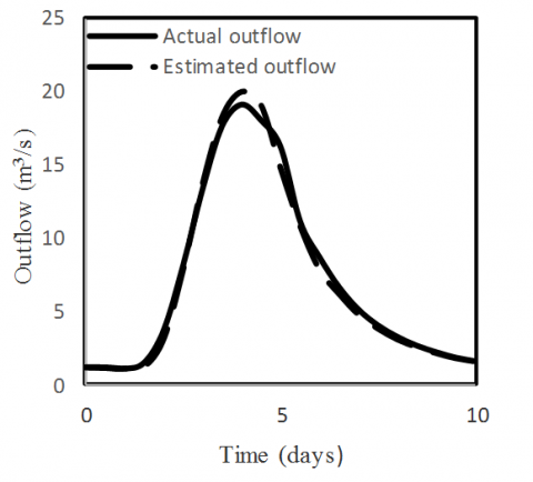
Figure 2. Actual and estimated outflow relationship for Trial and Error method
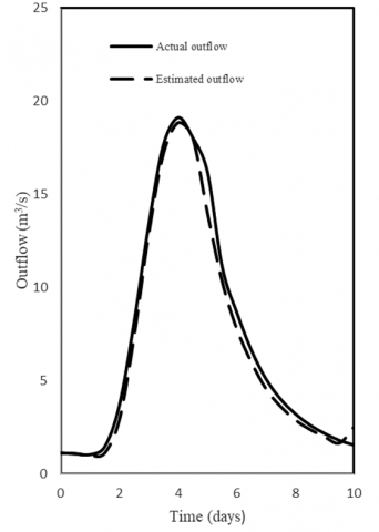
Figure 3. Actual and estimated outflow relationship for Least Square method with c=0

Figure 4. Actual and estimated outflow relationship for Least Square method with c≠0
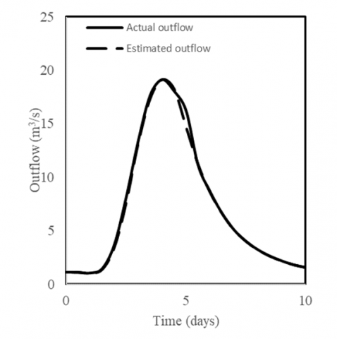
Figure 5. Actual and estimated outflow relationship for Direct Optimization method (DO)
The data for the nonlinear model is given in table 3.
Table 3. Actual inflow and outflow data for nonlinear model*
|
Time (Hours) |
Inflow (m3/s) |
Outflow (m3/s) |
|
0 |
0.623 |
0.623 |
|
6 |
0.651 |
0.594 |
|
12 |
0.991 |
0.594 |
|
18 |
2.009 |
0.736 |
|
24 |
2.915 |
0.962 |
|
30 |
3.141 |
1.245 |
|
36 |
3.085 |
1.557 |
|
42 |
2.830 |
1.868 |
|
48 |
2.434 |
2.123 |
|
54 |
2.009 |
2.321 |
|
60 |
1.670 |
2.406 |
|
66 |
1.330 |
2.377 |
|
72 |
1.104 |
2.264 |
|
78 |
0.906 |
2.066 |
|
84 |
0.792 |
1.811 |
|
90 |
0.679 |
1.528 |
|
96 |
0.623 |
1.245 |
|
102 |
0.594 |
1.019 |
|
106 |
0.566 |
0.849 |
|
114 |
0.538 |
0.708 |
|
120 |
0.538 |
0.623 |
|
126 |
0.509 |
0.538 |
*[19]
The parameters K and x, and various statistics are carried out as explained earlier and the results are shown in table 4.
Table 4. Parameter estimation and comparative statistics for the nonlinear method
|
Parameter Estimates |
DPO (m3/s) |
DPOT (hrs) |
Res Var (m3/s2) |
||
|
x |
K |
n |
|||
|
0.215 |
0.0548 |
2.352 |
0.073 |
0 |
0.297 |
Figure 6. Actual and estimated outflow relationship for Nonlinear method
Three methods (Trial and Error, Least Square and Direct Optimization) based on the linear model were investigated and used. It is clear that both the Least Squares and Trial and Error methods yield very close values in x and K.
The Direct Optimization method yields different values for x and K when compared with the other methods. However, it appears to be the most accurate of all since it gives the minimum DPO and residual variance. Three points emerge from the analysis of the above data. First, the three methods are comparable in their results on the whole. Second, although K and x are significantly different for these models, they lead to more or less comparable outflow hydrographs. This suggests that there might exist more than one set of the parameters K and x for the Muskingum flood routing method. Third, the direct linear optimization method is simple to apply and avoids the intermediate step of obtaining K and x.
Comparability of the results indicates that there is no particular reason to use the trial and error graphical method. Because the trial and error graphical approach, which have been used for decades, is time consuming and prone to subjective interpretation. Therefore, there exists little reason to use the graphical methods as practiced currently.
The value of K in the nonlinear method is associated with inflow and outflow, Δt in hours and n = 2.352 only. The results suggest a very good fit for the estimated values to the actual values, for both the linear and nonlinear method.
[1] McCarthy, G.T. (1938). The Unit Hydrograph and Flood Routing. Presented at Conference of North Atlantic Division, U.S. Army Corps of Engineers.
[2] Gill, M.A. (1978). Flood routing by Muskingum method. Journal of Hydrology, 36: 353-363. http://dx.doi.org/10.1016/0022-1694(78)90153-1
[3] Karahan, H., Gurarslan, G., Geem, Z.W. (2013). Parameter estimation of the nonlinear Muskingum flood-routing model using a hydbrid harmony search algorithm. Journal of Hydrologic Engineering, 18(3): 49-54. http://dx.doi.org/10.1061/(ASCE)HE.1943- 5584.0000608
[4] Fenton, J. (2019). Flood routing methods. Journal of Hydrology, 570: 251-264. http://dx.doi.org/10.1016/j.jhydrol.2019.01.006
[5] Yoon, J., Padmanabhan, G. (1993). Parameter estimation of linear and nonlinear Muskingum models. Journal of Water Resource, ASCE, 119(5): 600-610. http://dx.doi.org/10.1061/(ASCE)0733-9496(1993)119:5(600)
[6] Reggiani, P., Todini, E. (2018). On the validity range and conservation properties of diffusion analogy and variable parameter Muskingum. Journal of Hydrology, 563: 167-180. http://dx.doi.org/10.1016/j.jhydrol.2018.05.053
[7] Stephenson, D. (1979). Direct optimization of Muskingum routing coefficients. Journal of Hydrology, 41: 161-165. http://dx.doi.org/10.1016/0022-1694(79)90115-X
[8] Gill, M.A. (1979). Critical examination of the Muskingum method. Nordic Hydrology Research, 10: 361-370. http://dx.doi.org/10.2166/nh.1979.0009
[9] Cunge, J.A. (1969). On the subject of a flood propagation computation method (Muskingum Method). Journal of Hydrology Research, 7(2): 205-230.
[10] Singh, V.P., McCann, R.C. (1979). Quick estimation of parameters of Muskingum method of flood routing. Proc. 14th Annual Mississippi Water Resource. Conference, Jackson, Mississippi, USA, pp. 65-70.
[11] Barbetta, S., Coccia, G., Moramarco, T., Todini, E. (2018). Real-time flood forecasting downstream river confluences using a Bayesian approach. Journal of Hydrology, 565: 516-523. http://dx.doi.org/10.1016/j.jhydrol.2018.08.043
[12] Alhumoud, J.M., Esen, I.I. (2006). Approximate methods for the estimation of Muskingum flood routing parameters. Water Resources Management, 20(6). http://dx.doi.org/10.1007/s11269-006-9018-2
[13] Singh, V., McCann, R. (1980). Some notes on Muskingum method of flood routing. Elsevier Scientific Publishing Co., 333-361. http://dx.doi.org/10.1016/0022-1694(80)90125-0
[14] Kim, D. (2018). High-spatial-resolution streamflow estimation at ungauged river sites or gauged sites with missing data using the National Hydrography Dataset (NHD) and U.S. Geological Survey (USGS) streamflow data. Journal of Hydrology, 565: 819-834. http://dx.doi.org/10.1016/j.jhydrol.2018.08.074
[15] Munar, A., Cavalcanti, J., Bravo, J., Fan, F., Fragoso, C. (2018). Coupling large-scale hydrological and hydrodynamic modeling: Toward a better comprehension of watershed-shallow lake processes. Journal of Hydrology, 564: 424-441. http://dx.doi.org/10.1016/j.jhydrol.2018.07.045
[16] Yazdi, J., Sadiq, M., Neyshabourni, S., Gharahbagh, A. (2018). Assessment of different MOEAs for rehabilitation evaluation of Urban Stormwater Drainage Systems – Case study: Eastern catchment of Tehran. Journal of Hydro-environment Research, 21: 76-85. http://dx.doi.org/10.1016/j.jher.2018.08.002
[17] Guang, W., Singh, V. (1992). Muskingum method with variable parameters for flood routing in channels. Journal of Hydrology, 134: 57-76. http://dx.doi.org/10.1016/0022-1694(92)90028-T
[18] Linsley, R.K., Kohler, M.A., Paulhus, J.L.H. (1958). Hydrology for Engineers. McGraw-Hill Book Company, New York, 340.
[19] Wilson, E.M. (1990). Engineering Hydrology. MacMillan Book Co., London, England. http://dx.doi.org/10.1007/978-1-349-11522-8