Ravichandra Nayakar | Ulavathi Shettar Mahabaleshwar* | Poorigaly Nanjundaswamy Vinaykumar | Giulio Lorenzini | Dumitru Baleanu
OPEN ACCESS
The main objective of this article is to explore analytical solution for fourth order highly nonlinear differential equation. The stretching/shrinking is a non-linear (at least quadratic) function along the direction of stretching/shrinking. The stretching/ shrinking of a sheet with a velocity profiles are comparatively dependent on the distance from the velocity axes. The system of partial differential equations is transformed into the system of highly nonlinear ordinary differential equation via similarity transformation. Velocity profiles as a function of stretching/shrinking related parameters, Chandrasekhar number and viscoelastic parameter are discussed graphically. The analytical solutions of system of boundary layer equations emerging from the stretching/shrinking sheet problems were investigated and also the outcomes are in good agreement with the classical results on this topic. The outcomes have conceivable mechanical applications in fluid based frameworks including stretchable materials, in polymer extrusion process, metal spinning and other industrial processes.
non-linear stretching/shrinking sheet, Walters’ liquid B, analytical solution, magnetic field, fourth order non-linear differential equation
In past decades there has been voluminous amount of research work has taken place on the steady, laminar, boundary layer flows over stretching/shrinking sheet as it is routinely experienced in various outlining orders, such as polymer removal, drawing of copper wires, continuous extension of plastic movies, counterfeit strands, hot moving glass foils, metal extrusions and metal turning are the few cases where the issue of a stretching/shrinking sheet emerges. Magnetohydrodynamic (MHD) flows are significantly applicable in metallurgical industry, in the processes like cooling of consistent strips and strands passing through quiescent liquid, the filtration of liquid metals from non-metallic unions and other processes of such kind.
The leading the customary issue on steady laminar boundary layer flow due to the linear stretching sheet as discussed in Sakiadis [1], starting there, Crane's work has connected by Sakiadis [2], many works on these have appeared in different parts of the issue. Pavlov [3] contemplated the magnetohydrodynamics (MHD) flow of an electrically directing liquid because of a stretching sheet within the sight of a transverse magnetic field but he neglected the induced magnetic field under the assumed presence of little magnetic Reynolds number. Siddappa and Abel [4] have examined non-Newtonian fluid flow past a stretching plate and gave analytical solutions and further, same problem has been extended by Mahabaleshwar and Lorenzini [5] inclusion of nonlinear stretching/shrinking sheet in the presence of MHD. This problem was further extended by Ariel [6] by taking into account of MHD with suction. Andersson [7], discussed the MHD flow of a viscoelastic fluid flow past a stretching sheet and obtained the exact analytical solutions of a nonlinear laminar, steady boundary layer equation. He has shown that the influence of external MHD has the same effect as that of the viscoelasticity on the fluid. The heat transfer of viscoelastic fluid flow in a saturated porous medium has been analysed using Kummer’s function by Pillai et. al [8]. They have carried out the analysis by considering prescribed heat transfer case as well as based on prescribed heat flux case. Exact analytical solutions for velocity field and skin-frictions are obtained by them. Siddeshwar and Mahabaleshwar [9] studied the effects of radiation and heat source on MHD flow of a viscoelastic liquid and heat transfer over a stretching sheet and obtained exact analytical solutions for velocity profiles and heat transfer by applying Kummer’s function. This was further extended by Mastroberardino and Mahabaleshwar [10] by considering the viscoelastic fluid flow due to a stretching sheet in a porous medium in mixed convection and obtained the analytical solutions via homotopy analysis method. In 2017, Mabood et al. [11] have discussed radiation effects on Williamson nanofluid flow over a heated surface with magnetohydrodynamics. The centre suspicion in a large portion of the reported issues is that the stretching is non-linearly relative to the axial distance. This is substantial given the stretching procedure is fragile and moderate, prompting the suspicion of constant rate of stretching. It is not hard to see that the above supposition is very hopeful and unrealistic. Verifiable in this is certainty that the stretching must be carefully ease back to guarantee such a presumption. Basically, direct stretching sheet is difficult to acknowledge, if unrealistic. In the strictest sense the stretching must be nonlinearly corresponding to the axial distance.
Now a day, the interest has been connected with the issue of flow over both stretching/shrinking sheets in the presence of MHD with suction/injuction. This sort of issue is of particular importance as the flow is contracted towards a slit that would bring about speed far from the sheet. Here, the development of the sheet in inverse (negative x-axis) direction to the stretching sheet, along these lines driven by a stretching/shrinking sheet, and this kind of stretching/shrinking flow is basically a reverse flow.
The present work is a gives the analytical solution by considering the frameworks set up by Siddheshwar and Mahabaleshwar [9], Mastroberardino and Mahabaleshwar [10] for a linear stretching sheet and in fact, here in addition to the stretching sheet case, the results are also obtained for shrinking sheet case. The physical properties of the fluid flow are greatly influenced by the presence of the stretching/shrinking parameter, which pushes it into the non-linear category. In the present paper, as an initial phase in the general nonlinear demonstrating exercise, we make usage of a basic quadratic stretching/shrinking model.
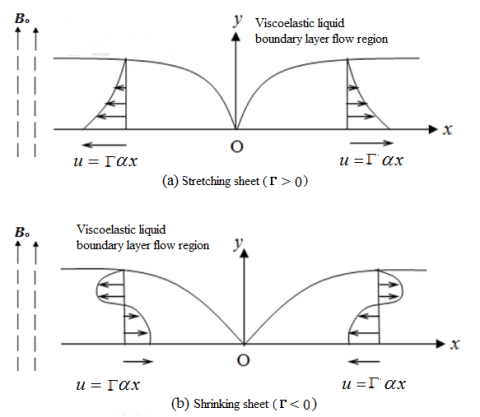
The two-dimensional steady, laminar, boundary layer flow of an electrically conducting non-Newtonian fluid, of the form Walters’ liquid B, over a non-linear stretching/shrinking sheet (see Figure 1a, b). The Walters' liquid B addresses a supposition for short or rapidly obscuring memory fluids and is along these lines estimation to first order in elasticity. Initially, the liquid is at rest and motion is brought into it by pulling the sheet on both extremes with equivalent forces parallel to the sheet and with a speed u, which differs non-linear with the separation from the slit as u=αx+βx2. The subsequent movement of the generally quiescent liquid is in this manner brought about exclusively by the moving sheet, assuming β, and thereby δ, quite small we can make use of the boundary layer theory [9, 10].
$\frac{\partial u}{\partial x}+\frac{\partial v}{\partial y}=0$ (1)
$\begin{align} & u\frac{\partial u}{\partial x}+\text{v}\frac{\partial \text{v}}{\partial y}=\nu \frac{{{\partial }^{2}}u}{\partial {{y}^{2}}}-\frac{\sigma B_{0}^{2}}{\rho }u \\ & \,\,\,\,\,\,\,\,\,\,\,\,\,\,-{{k}_{0}}\left\{ u\frac{{{\partial }^{3}}u}{\partial x\partial {{y}^{2}}}+\text{v}\frac{{{\partial }^{3}}u}{\partial {{y}^{3}}}+\frac{\partial u}{\partial x}\frac{{{\partial }^{2}}u}{\partial {{y}^{2}}}-\frac{\partial u}{\partial y}\frac{{{\partial }^{2}}u}{\partial x\partial y} \right\} \\ \end{align}$ (2)
The boundary conditions for the non-linear stretching/shrinking sheet are given underneath:
$\left. \begin{align} & u=\Gamma \left( \alpha x+\beta {{x}^{2}} \right)\text{at}y=0, \\ & \text{v}=\delta x\text{at}y=0, \\ & u=0\text{as}y\to \infty .\,\,\,\,\, \\ \end{align} \right\}$ (3a, b, c)
where, u and v are parts of the fluid speed in the longitudinal axis and transverse axis, individually, Г is the stretching /shrinking sheet coefficient with Г>0 stretching sheet rate and Г<0 shrinking sheet rate, for remaining notations can be referred from listed nomenclature.
Utilizing dimensionless variables for non-linear stretching/shrinking model in our problem
$(X,Y)=\sqrt{\frac{\alpha }{\nu }}(x,y),\,\,(U,V)=\frac{(u,v)}{\sqrt{\alpha \nu }},{{\beta }^{*}}=\frac{\beta }{\alpha }\sqrt{\frac{\nu }{\alpha }},{{\delta }^{*}}=\frac{\delta }{2\alpha },$ (4)
Eqns. (1) and (2) take the structure
$\frac{\partial U}{\partial X}+\frac{\partial V}{\partial Y}=0$ (5)
$\begin{align} & U\frac{\partial U}{\partial X}+V\frac{\partial V}{\partial Y}=\frac{{{\partial }^{2}}U}{\partial {{Y}^{2}}}-QU \\ & \,\,\,-{{k}_{1}}\left\{ U\frac{{{\partial }^{3}}U}{\partial X\partial {{Y}^{2}}}+V\frac{{{\partial }^{3}}U}{\partial {{Y}^{3}}}+\frac{\partial U}{\partial X}\frac{{{\partial }^{2}}U}{\partial {{Y}^{2}}}-\frac{\partial U}{\partial Y}\frac{{{\partial }^{2}}U}{\partial X\partial Y} \right\} \\ \end{align}$ (6)
where, ${{k}_{1}}=\frac{\alpha \ {{k}_{0}}}{\mu }$ is the viscoelastic parameter and $Q\,=B_{0}^{2}\frac{\sigma \,}{\alpha \rho }$ is the Chandrasekhar number ($\sqrt{Q\,}$ is called Hartmann number). Due to the Hartman formulation, the boundary conditions of magnetic field do not affect the dynamics of the fluid.
Presenting the physical stream function$\psi (X,Y)$, as
$U=\frac{\partial \psi }{\partial Y},\,\,\,\,\,\,V\ =\ \ -\ \ \frac{\partial \psi }{\partial X}$ (7)
Utilizing Eq. (7) in Eq. (6), we get
$\begin{align} & \frac{{{\partial }^{3}}\psi }{\partial {{Y}^{3}}}+\frac{\partial \left( \,\psi ,\,\,\,\frac{\partial \psi }{\partial Y}\, \right)}{\partial \left( \,X,\,Y \right)}\,+Q\frac{\partial \psi }{\partial Y} \\ & +{{k}_{1}}\,\left\{ \,\frac{\,\partial \left( \,\psi ,\,\,\,\frac{{{\partial }^{3}}\psi }{\partial {{Y}^{3}}} \right)}{\partial \left( \,X,\,Y \right)}-\frac{\partial \left( \,\frac{\partial \psi }{\partial Y},\,\,\,\frac{{{\partial }^{2}}\psi }{\partial {{Y}^{2}}} \right)}{\partial \left( \,X,\,Y \right)} \right\}=\,0 \\ \end{align}$ (8)
In Eq. (8), second and third term denote the Jacobians. Using Eqns. (3), (4) and (7), ψ fulfils the following boundary conditions:
$\left. \begin{matrix} \frac{\partial \psi }{\partial Y}=\Gamma \left( X+{{\beta }^{*}}{{X}^{2}} \right)\,\,\,\,\,\,\,\,\,\,\,\,\,\,\text{at}\,\,\,\,Y=0 \\ \frac{\partial \psi }{\partial X}=-2\,{{\delta }^{*}}X\,\,\,\,\,\,\,\,\,\,\,\,\,\,\,\,\,\,\,\,\,\,\,\,\,\,\,\text{at}\,\,\,\,Y=0\,\,\, \\ \frac{\partial \psi }{\partial Y}=0\,\,\,\,\,\,\,\,\,\,\,\,\,\,\,\,\,\,\,\,\,\,\,\,\,\,\,\,\,\,\,\,\,\,\,\,\,\,\,\,\,\,\,\,\text{at}\,\,\,\,Y\to \infty \\ \end{matrix} \right\},$ (9a, b, c)
The similarity solution for Eq. (8), subject to Eq. (9a, b, c), might be taken as
$\psi =Xf(Y)-{{\delta }^{*}}{{X}^{2}}{{f}_{Y}}(Y)$ (10)
where, subscripts indicate derivative with respect to Y. Using equations (8) and (10) and likening the coefficients of X, X2, and X23, we get the following three highly nonlinear ordinary differential equations:
$\begin{align} & {{\left( {{f}_{Y}} \right)}^{2}}-f\,{{f}_{YY}}={{f}_{YYY}}-Q{{f}_{Y}} \\ & \,\,\,\,\,\,\,\,\,\,\,\,\,\,\,\,\,\,\,\,\,\,\,\,\,\,\,\,\,\,\,\,\,\,\,\,\,\,\,\,\,-{{k}_{1}}\left\{ 2{{f}_{Y}}{{f}_{YYY}}-f\,{{f}_{YYYY}}-{{\left( {{f}_{Y}} \right)}^{2}} \right\} \\ \end{align}$ (11)
$\begin{align} & {{f}_{Y}}{{f}_{YY}}-f{{f}_{YYY}}={{f}_{YYYY}}-Q{{f}_{YY}} \\ & \,\,\,\,\,\,\,\,\,\,\,\,\,\,\,\,\,\,\,\,\,\,\,\,\,\,\,\,\,\,\,\,\,\,\,\,\,\,\,\,\,\,\,\,\,\,-{{k}_{1}}\left\{ {{f}_{Y}}{{f}_{YYYY}}-f{{f}_{YYYYY}} \right\} \\ \end{align}$ (12)
and
$\begin{align} & {{\left( {{f}_{YY}} \right)}^{2}}-{{f}_{Y}}{{f}_{YYY}} \\ & \,\,\,\,\,\,\,\,\,\,\,\,\,\,\,\,\,\,\,={{k}_{1}}\left\{ {{f}_{Y}}{{f}_{YYYYY}}-2{{f}_{YY}}{{f}_{YYYY}}+{{\left( {{f}_{YYY}} \right)}^{2}} \right\} \\ \end{align}$ (13)
Condition (12) turns out repetitive as it can be acquired by differentiating g Eq. (11) once as for Y. In the subsequent investigation we demonstrate that Eq. (11) can, actually, be got from Eq. (13), by an appropriate transformation, which thus suggests consistency.
The boundary conditions for unravelling Eq. (11) in f, is given by Eqns. (9a, b, c) can be gotten in the structure,
$\left. \begin{align} & {{f}_{Y}}(0)=\Gamma ,\ \ {{f}_{YY}}(0)=-\ s,\ \ \\ & f(0)=0, \\ & {{f}_{Y}}(\infty )=0,\ {{f}_{YY}}(\infty )=0,\ \\ \end{align} \right\}$ (14a, b, c)
where, $s=\frac{{{\beta }^{*}}}{{{\delta }^{*}}}$, Г>0 is the stretching sheet parameter and Г<0 is the shrinking sheet parameter. One can easily see that Eq. (13) is a differential equation for fY and we can also verify that ${{f}_{Y}}={{e}^{-sY}}$ is a solution of Eq. (13) and this satisfies the derivative boundary conditions in Eq. (14). ${{f}_{Y}}(\infty )\to 0$, the physical solution ${{f}_{Y}}(\infty )\to 0$ must also satisfy the condition ${{f}_{Y}}(\infty )\to 0$ of smooth asymptotic decay. Thus an appropriate solution of Eq. (11) is
$f(Y)=A+B\,e{{}^{-sY}}\,$ (15)
which satisfy the boundary condition (14) provided,
$A=\frac{{{\delta }^{*}}}{{{\beta }^{*}}}\,\,\text{, }\,B=-\frac{{{\delta }^{*}}}{{{\beta }^{*}}}\,\,\,\,\text{and}\,\,\,s=\tfrac{1}{A}$ (16)
The solution of the highly nonlinear ordinary differential equation (11) is that Eq. (15) if and only if,
$s=\frac{{{\beta }^{*}}}{{{\delta }^{*}}}=\Gamma \sqrt{\frac{1+Q}{1-{{k}_{1}}}}$ (17)
We may now write f(Y) from Eqs. (15)- (17) as follows:
$f(Y)=\Gamma \left[ \frac{1-\exp \left( -\,\,sY \right)}{s} \right]$ (18)
Using this in Eq. (13), we can arrive at Eq. (11). This proves the “consistency” of the equations (11)-(13) in f.
The expression for the streamline pattern of the flow in the region around the stretching sheet can be obtained from Eq. (10) as:
$\psi =X\,f-{{\delta }^{*}}{{X}^{2}}{{f}_{Y}}=C$ (19)
where, C is a constant. The streamline ψ=C can be written in the functional form as
$Y=\frac{\Gamma }{s}\,\,\left[ Ln\ \left\{ \,\frac{\frac{X}{s}+{{\delta }^{*}}{{X}^{2}}}{\frac{X}{s}-C} \right\} \right]$ (20)
Substituting Eq. (10) into Eq. (7), we get the following expressions for dimensionless axial as well as transverse velocity profiles,
$U=\Gamma \left[ X\,{{f}_{Y}}-{{\delta }^{*}}{{X}^{2}}\,{{f}_{YY}} \right]$ (21)
$V=\Gamma \left[ -f+2{{\delta }^{*}}X\,\,{{f}_{Y}} \right]$ (22)
Having obtained the analytical expression for the stream function ψ and the axial velocity U and transverse velocity V, we now discuss the results obtained above.
Table 1. List of the previous works on the expressions of β for different stretching/shrinking sheet
|
Related works by other authors |
Fluids |
Value of b |
|
Crane [1], Viscous fluid with suction /injection and without MHD, stretching sheet |
Newtonian |
β=1 |
|
Pavlov [3], Incompressible viscous fluid with MHD, stretching sheet without suction/ injection |
Newtonian |
$\beta =\sqrt{\left( 1+Q \right)}$ |
|
Gupta and Gupta [12], Viscous fluid with heat and mass transfer with suction/injection, stretching sheet |
Newtonian |
$\beta =\frac{-{{V}_{C}}+\sqrt{V_{C}^{2}+4\left( 1+Q \right)}}{2}$ |
|
Dandapat et al. [13], Non-Newtonian electrically conducting fluid, stretching sheet |
Non-Newtonian |
$\beta =\frac{-{{V}_{C}}+\sqrt{V_{C}^{2}+4\left( 1+Q \right)}}{2}$ |
|
Siddappa and Abel [4], Non-Newtonian fluid with suction, stretching sheet |
Non-Newtonian |
Minimum of positive roots of $\left( {{V}_{C}}\beta -1 \right)\left( 1+{{k}_{1}}{{\beta }^{2}} \right)+{{\beta }^{2}}=0$ |
|
Ariel [6], Viscoelastic fluid with MHD, stretching sheet with suction |
Non-Newtonian |
Minimum of positive roots of $\left( {{V}_{C}}\beta -1 \right)\left( 1+{{k}_{1}}{{\beta }^{2}} \right)+\left( {{\beta }^{2}}-Q \right)=0$ |
|
Siddheshwar and Mahabaleshwar [9], Viscoelastic fluid with MHD and heat transfer, stretching sheet |
Non-Newtonian |
$\beta =\sqrt{\frac{1+Q}{1-{{k}_{1}}}}$ |
|
Siddheshwar et al. [14], Viscoelastic fluid with MHD and suction, stretching sheet within porous medium |
Non-Newtonian |
$\left( {{V}_{C}}\beta -1 \right)\left( 1+{{k}_{1}}{{\beta }^{2}} \right)+\left( {{\beta }^{2}}-Q-K \right)=0$ |
|
present work |
Non-Newtonian |
$\beta =\frac{{{\beta }^{*}}}{{{\delta }^{*}}}=\Gamma \sqrt{\frac{1+Q}{1-{{k}_{1}}}},\,$ where, Г is the stretching/ shrinking sheet parameter |
Figure 1. Schematic diagram of the stretching/shrinking sheet problem
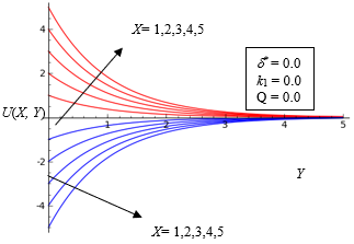
Figure 2. Axial velocity for the linear stretching/shrinking sheet problem of Crane (1970) and in the absence of non-linear
Figure 3. Axial velocity U(X,Y) for the linear stretching/shrinking sheet problem of Crane (1970)
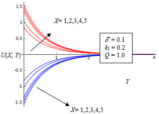
Figure 4. Axial velocity U(X,Y) for the non-linear (at least quadratic) stretching/shrinking sheet problem
In this paper, we investigated results on the viscoelastic fluid past a non-linear stretching/shrinking sheet. Mathematical modelling of the boundary layer with the governing equations, gives rises to highly non-linear ordinary differential equations (11)-(13) which are solved analytically subjected to non-linear stretching/shrinking conditions. The flow generated by the flexible sheet after undergoing non-linear stretching/shrinking in its neighbourhood is investigated and it establishes that the stretching/shrinking sheet is the main cause for the fluid flow, and also the significant influence of viscoelasticity of the fluid. Here we consider the Walters’ liquid B, a special class of non-Newtonian fluid and it is also a non-linear stretching/shrinking sheet in the presence of transverse magnetic field. Similarity solution is obtained for the velocity distribution. The dimensionless velocity profiles U and V are both decreasing functions of Y as it is an exponential function with negative contentions. From Eq. (17), it is clear that the slope of exponentially decreasing velocity component is influenced by suction parameter ‘s’, a function of the Chandrasekhar number Q. Hence,‘s’ plays an important role in the behaviour of the flow problem. The flow of MHD liquid, inhibited by a transverse magnetic field, is investigated with the help of streamline patterns and also the velocity distributions. These results are analyzed against the background of the classical linear stretching problem δ*=0 involving Newtonian fluids k1=0 and Q = 0 (see [1]). It is evident from the equation (17) that the k1 range of applicability of the solution is (-∞, 1). This is substantiated by the differentiating the Eq.(11) with respect to Y, and subject to condition (14), gives
${{f}_{YY}}(0)=\left( \frac{1-{{k}_{1}}}{1+Q} \right)\,\,{{f}_{YYYY}}(0)$ (23)
From the Eq. (23), one can see that $f_{YY}(0)=0$ for $k_1=1$. In conjunction with the condition $f_{YY}(0)=-s$ in equation (14a), this would mean,
$f_{YY}(0)=-s=0$ (24)
Obviously for k1=1, the quadratic stretching sheet problem ceases to exist. For k1>1 we note that $s=\sqrt{\frac{1+Q}{1-k_{1}}}$ is complex. Hence, it stands reiterated that the range of applicability of k1 must be (-∞, 1). The influence of Г the stretching/shrinking parameter on the present study is that when Г>0,we get stretching sheet case, when, Г<0 a shrinking sheet case and Г=0 for fixed surface.
Figure 2-4 is a plot of the streamline ψ(X,Y)=1 for various values of δ* with Q = 1 and k1=0.2. Increasing value of δ* indicates the increasing rate of non-linear stretching/shrinking. It can find from the figure that increasing rate of stretching restricts the dynamics in the axial direction to regions close to the slit. It is evident from the figures that the Chandrasekhar number Q, viscoelastic parameter k1 and quadratic stretching parameter δ* work against each other in the lifting of the liquid as we go downstream, it is also evident that as we go along the sheet the vertical extent of the fluid that is shaken up from inertia, increases with axial distance. This is due to the fact that when the stretching/shrinking is non-linear the response of the fluid to the stretching/shrinking does not match. Thus, it forces us to go along with transverse directions. The effect of k1, Q, δ* and Г parameters on axial velocity at the surface increasing with non-linear stretching velocity and decrease with non-linear shrinking velocity. The thickness of hydrodynamic laminar boundary layer also depends upon the Г. The thickness of the boundary layer sheet is larger for a shrinking sheet than a stretching sheet and the effects of Q are well-defined.
A, B, C constants
B0 magnetic field (T-Tesla)
f similarity function for velocity
k0 viscoelastic constant
k1 viscoelastic parameter$\left( ={\alpha {{k}_{0}}}/{\mu }\; \right)$
u velocity component along x-axis ( m s-1)
v velocity component along y-axis (m s-1)
x axial axis (m)
y transverse axis (m)
Greek symbols
α,β constants rate of stretching/shrinking (s-1)
β* nonlinear stretching/shrinking (s-1)
σ electrical conductivity
μ viscosity (kg m-1s-1)
v kinematic viscosity, $\left( ={\mu }/{\rho }\; \right)$ (m2 s-1)
ρ density (kgm-3)
Г stretching/shrinking coefficient
ψ physical stream function (m2 s-1)
δ constant (s-1)
δ* nonlinear parameter
Subscripts/Superscripts
0 pole
w wall condition
∞ far from the sheet
* dimensionless quantities
fY first order derivative with respect to Y
fYY second order derivative with respect to Y
fYYY third order derivative with respect to Y
fYYYY fourth order derivative with respect to Y
[1] Crane, L.J. (1970). Flow past a stretching plate. ZAMP, 21: 645-647. https://doi.org/ 10.1007/BF01587695
[2] Sakiadis, B.C. (1961). Boundary-layer behavior on continuous solid surfaces II. The boundary layer on a continuous flat surface. AIChE J., 7: 221. https://doi.org/10.1002/aic.690070211
[3] Pavlov, K.B. (1974). Magnetohydrodynamic flow of an incompressible viscous liquid caused by deformation of plane surface. Magnetnaya Gidrodinamica, 4: 146. https://doi.org/10.22364/mhd
[4] Siddappa, B., Abel, M.S. (1985). Non-Newtonian flow past a stretching plate. Zeitschrift für Angewandte der Mathematik und Physik (ZAMP), 35: 1-3. https://doi.org/10.1007/BF00944900
[5] Mahabaleshwar, U.S., Lorenzini, G. (2017). Combined effect of heat source/sink and stress work on MHD Newtonian fluid flow over a stretching porous sheet. International Journal of Heat and Technology, 35: S330-S335. https://doi.org/10.18280/ijht.35Sp0145
[6] Ariel, P.D. (1994). MHD flow of a viscoelastic fluid past a stretching sheet with suction. Acta Mechanica, 105: 49-54. https://doi.org/10.1007/BF01183941
[7] Andersson, H.I. (1992). MHD flow of a viscoelastic fluid past a stretching surface. Acta Mech., 95: 227. https://doi.org/10.1007/BF01170814
[8] Pillai, K.M.C., Sai, K.S., Swamy, N.S., Nataraja, H.R., Tiwari, S.B., Rao, B.N. (2004). Heat transfer in a viscoelastic boundary layer flow through a porous medium. Computational Mechanics, 34: 27-37. https://doi.org/10.1007/s00466-004-0550-8
[9] Siddheshwar, P.G., Mahabaleshwar, U.S. (2005). Effects of radiation and heat source on MHD flow of a viscoelastic liquid and heat transfer over a stretching sheet. International Journal of. Nonlinear Mechanics, 40: 807. https://doi.org/10.1016/j.ijnonlinmec.2004.04.006
[10] Mastroberardino, A., Mahabaleshwar, U.S. (2013). Mixed convection in viscoelastic flow due to a stretching sheet in a porous medium. Journal of Porous Media, 16(6). https://doi.org/10.1615/JPorMedia.v16.i6
[11] Mabood, F., Ibrahim, S.M., Lorenzin, G., Lorenzini, E. (2017). Radiation effects on Williamson nanofluid flow over a heated surface with magnetohydrodynamics. International Journal of Heat and Technology, 35(1): 196-204. https://doi.org/10.18280/ijht.350126
[12] Gupta, P.S., Gupta, A.S. (1977). Heat and mass transfer on a stretching sheet with suction or blowing. Canadian Journal of Chemical Engineering, 55: 744-746. https://doi.org/10.1002/cjce.5450550619
[13] Dandapat, B.S., Holmedal, L.E., Andersson, H.I. (1994). On the stability of MHD flow of a viscoelastic fluid past a stretching sheet. Arch. Mech., 130: 143-149. https://doi.org/10.1007/BF01187050
[14] Siddheshwar, P.G., Mahabaleshwar, U.S., Chan, A. (2014). Suction-induced MHD of a viscoelastic fluid over a stretching surface within a porous medium. IMA Journal of Applied Mathematics, 79(3): 445-458. https://doi.org/10.1093/imamat/hxs074
[15] Vleggaar, J. (1977). Laminar boundary-layer behaviour on continuous accelerating surfaces. Chem. Eng. Sci., 32(12): 1517. https://doi.org/10.1016/0009-2509(77)80249-2