Darbhashayanam Srinivasacharya* | Pashikanti Jagadeeshwar
OPEN ACCESS
Laminar slip flow in a Darcy-Brinkman porous medium saturated with incompressible viscous fluid over an exponentially stretching sheet with double dispersion effects is considered. The influence of thermal radiation is taken into account. The governing non-dimensional equations are transformed into coupled ordinary non-linear differential equations using local similarity and non-similarity method. The resulting systems of equations are solved using the successive linearization method together with the Chebyshev pseudo spectral method. The salient features of the investigation on the development of the flow, temperature, concentration, heat and mass transfer are discussed and displayed through graphs.
double dispersion, porous medium, convective thermal condition, heat and mass transfer
The investigation of flow over a sheet stretching exponentially is of considerable interest because of its applications in industrial and technological processes, such as, fluid film condensation process, crystal growth, aerodynamic extrusion of plastic sheets, the cooling process of metallic sheets, design of chemical processing equipment and various heat exchangers and glass and polymer industries. The pioneering works of Sakiadis [1, 2] motivated the several, researchers to investigate the flow due to stretching sheet.
Influence of thermal radiation on heat transfer phenomenon has several applications in many technological processes, including various propulsion devices for aircraft, gas turbines, nuclear power plants, satellites, missiles and space vehicles. Pramanik [3] explored the thermal radiation on heat transfer analysis towards a stretching surface in presence of fluid suction or blowing at the surface. Yasir et al. [4] reported the radiative heat transfer analysis of the boundary layer flow towards exponentially shrinking sheet. Remus and Marinca [5] presented the MHD viscous fluid flow over a porous sheet stretching exponentially with thermal radiation. Krupalakshmi et al. [6] studied the influence of thermal radiation on the flow of a dusty non-Newtonian fluid over a stretching surface. Khan et al. [7] investigated the influence solar radiation on the flow of a Carreau nanofluid induced by a stretching sheet. Mabood et al. [8] reported that raising Prandtl number escalates the rate of heat transfer. Thirupathi et al. [9] numerically investigated the radiative MHD flow a nanofluid over an inclined stretching sheet.
Generally accepted boundary condition on the solid surface is no-slip condition. However, Navier [10] suggested that fluid slips at the solid boundary and slip velocity depends linearly on the shear stress. The fluid slippage phenomenon at the solid boundary appear in numerous applications, for example, in nanochannels or microchannels and the cleaning of simulated heart valves, internal cavities. Using this velocity-slip condition, Hayat et al. [11] investigated the flow and heat transfer analysis of MHD three dimensional flow over a stretching surface by taking thermal slip into the consideration. Ullah et al. [12] reported the effect of slip condition on the MHD flow induced by a nonlinear stretched surface. On the other hand, a novel technique for the heating process by providing the heat with finite capacity to the convecting fluid through the bounding surface has attracted by numerous researchers. This type of thermal boundary condition, called convective boundary condition, results in the rate of exchange of heat across the boundary being proportional to the difference in local temperature with the ambient conditions [13]. Due to the realistic nature of the convective thermal condition, the investigation of heat transfer with this condition has rich significance in mechanical and designing fields, for example, heat exchangers, atomic plants, gas turbines, and so forth. Further, heat transfer process in the boundary layers under convective thermal condition plays an important role in the processes such as nuclear plants, thermal energy storage, gas turbines, various propulsion devices for aircraft etc. Hayat et al. [14] investigated the importance convective type boundary conditions in modeling the heat transfer process of MHD flow of viscous nano-fluid over an exponentially stretching surface in porous medium. Rahman et al. [15] reported the steady flow, heat and mass transfer process of a nano-fluid past a permeable exponentially shrinking surface using the Buongiorno’s model. Khan et al. [16] analyzed the boundary layer flow of a nanofluid with convective thermal condition on past a bi-directional sheet stretching exponentially. Mustafa et al. [17] explored the rotational effects on the flow of a nanofluid over a sheet stretching exponentially with convective thermal condition. Srinivasacharya and Jagadeeshwar [18] investigated the slip flow of viscous fluid over a sheet stretching exponentially with convective thermal condition. Though, considerable literature available on stretched flow problem, but, as par as the author's knowledge, double dispersion effects together with thermal radiation on convective heat and mass transfer flow along a sheet stretching exponentially, considering the velocity slip at the stretching surface of the sheet is not analyzed so far.
Therefore, motivated by the aforementioned investigations, here we made an attempt to obtain the non-similar solutions of the flow and heat and mass transfer over an exponentially stretching surface in presence of thermal and solute dispersions. Furthermore, velocity slip at the surface of the sheet is taken into account.
Consider a sheet stretching exponentially in a Darcy-Brinkman porous medium saturated with incompressible viscous fluid with a temperature T∞ and concentration C∞. The Cartesian framework is selected by taking positive axis is along the sheet and axis is orthogonal to the sheet. The stretching velocity of the sheet is assumed as U*($\tilde{x}$) = U0 e/L where is the distance from the slit. Assume that the sheet is either cooled or heated convectively through a fluid with temperature Tf and which induces a heat transfer coefficient hf, where $\mathrm{h}_{\mathrm{f}}=\mathrm{h} \sqrt{U_{0} / 2 L}\mathrm{e}\tilde{x}^{\prime 2L}$. $u ̃_x,u ̃_y$ is the velocity vector, $C ̃$ is the concentration and is the temperature. The suction/injection velocity of the fluid through the sheet is $\mathrm{V} *(\tilde{x})=\mathrm{V}_{0} \mathrm{e}\tilde{x}^{/ 2\mathrm{L}}$, whereV0 is the strength of suction/injection. Further, the slip velocity of the fluid is assumed as $\mathrm{N}(\tilde{x})=\mathrm{N}_{0}\mathrm{e}-\tilde{x}^{/ 2L}$, where N0 is the velocity slip factor. The fluid is considered to be a gray, absorbing/emitting radiation, but non-scattering medium. The Rosseland approximation [19] is used to describe the radiative heat flux in the energy equation. Hence, the following are the equations which governs the present flow problem in presence of thermal, solutal dispersions and are given by:
$\frac{\partial \tilde{u}_{x}}{\partial \tilde{x}}+\frac{\partial \tilde{u}_{y}}{\partial \tilde{y}}=0$ (1)
$\tilde{u}_{x} \frac{\partial \tilde{u}_{x}}{\partial \tilde{x}}+\tilde{u}_{y} \frac{\partial \tilde{u}_{x}}{\partial \tilde{y}}=v \frac{\partial^{2} \tilde{u}_{x}}{\partial \tilde{y}^{2}}-\frac{v}{k_{p}} \tilde{u}_{x}$ (2)
$\tilde{u}_{x} \frac{\partial \tilde{T}}{\partial \tilde{x}}+\tilde{u}_{y} \frac{\partial \tilde{T}}{\partial \tilde{y}}=\frac{\partial}{\partial \tilde{y}}\left(\widetilde{\alpha}_{e} \frac{\partial \tilde{T}}{\partial \tilde{y}}\right)+\frac{16 T_{\infty}^{3} \sigma^{*}}{3 k^{*} \rho c_{p}} \frac{\partial^{2} \tilde{T}}{\partial \tilde{y}^{2}}$ (3)
$\tilde{u}_{x} \frac{\partial \tilde{C}}{\partial \tilde{x}}+\tilde{u}_{y} \frac{\partial \tilde{C}}{\partial \tilde{y}}=\frac{\partial}{\partial \tilde{y}}\left(\widetilde{D}_{e} \frac{\partial \tilde{C}}{\partial \tilde{y}}\right)$ (4)
where kP is the permeability of the porous medium, σ* is the Stefan-Boltzmann constant, k* is the mean absorption coefficient, υ, ρ and cp are kinematic viscosity, density and specific heat capacity at the constant pressure, respectively. The effective thermal and molecular diffusivities $\widetilde{{{\alpha }_{e}}}$ and $\widetilde{{{D}_{e}}}$ , respectively can be written as
$\widetilde{\alpha_{e}}=\alpha+\gamma u d, \widetilde{D_{e}}=D+\chi u d$ (5)
where α and D are thermal and molecular diffusiveness, γ and χ are coefficient of thermal and molecular diffusiveness which varies between 1/7 to 1/3 and d is pore diameter or mean particle diameter.
The conditions on the stretching surface are
$\tilde{u}_{x}=U_{*}+N v \frac{\partial \tilde{u}_{x}}{\partial \tilde{y}}, \tilde{u}_{y}=-V_{*}(\tilde{x})$
$h_{f}\left(T_{f}-\tilde{T}\right)=-\kappa \frac{\partial \tilde{T}}{\partial \tilde{y}}, \tilde{C}=C_{w}$ at $\tilde{y} \rightarrow 0$
$\tilde{u}_{x} \rightarrow 0, \tilde{T} \rightarrow T_{\infty}, \tilde{C} \rightarrow C_{\infty}$ as $\quad \tilde{y} \rightarrow \infty$$\}$ (6)
Introducing the stream functions through $\tilde{u}_{x}=-\frac{\partial \psi}{\partial \tilde{y}}$ and $\tilde{u}_{y}=\frac{\partial \psi}{\partial \tilde{x}}$ then the following dimensionless variables
$\tilde{x}=x L, \tilde{y}=y \sqrt{\frac{2 v L}{U_{0}}} e^{\frac{-\tilde{x}}{2 L}}, \psi=\sqrt{2 v L U_{0}} e^{\frac{\hat{x}}{2 L}} F(x, y),$
$\tilde{T}=T_{\infty}+\left(T_{f}-T_{\infty}\right) T(x, y), \tilde{C}=C_{\infty}+\left(C_{w}-C_{\infty}\right) C(x, y)$$\}$ (7)
and substituting (7) into Eqs. (1) – (4), we obtain
$F^{\prime \prime \prime}+F F^{\prime \prime}-2 F^{\prime 2}-K_{p} e^{-x} F^{\prime}+2\left(F^{\prime \prime} \frac{\partial F}{\partial x}-F^{\prime} \frac{\partial F^{\prime}}{\partial x}\right)=0$ (8)
$\frac{1}{P r}\left(1+\frac{4 R}{3}\right) T^{\prime \prime}+F T^{\prime}+2\left(T^{\prime} \frac{\partial F}{\partial x}-F^{\prime} \frac{\partial T}{\partial x}\right)+D_{\gamma} e^{x}\left(F^{\prime} T^{\prime \prime}+\right.$
$F^{\prime \prime} T^{\prime} )=0$ (9)
$\frac{1}{s c} C^{\prime \prime}+F C^{\prime}+2\left(C^{\prime} \frac{\partial F}{\partial x}-F^{\prime} \frac{\partial c}{\partial x}\right)+D_{\chi} e^{x}\left(F^{\prime} C^{\prime \prime}+F^{\prime \prime} C^{\prime}\right)=0$ (10)
The transformed boundary conditions are
$F(x, 0)+2 \frac{\partial F}{\partial x}(x, 0)=S, F^{\prime}(x, 0)=1+\lambda F^{\prime \prime}(x, 0),$
$T^{\prime}(x, 0)=-B i(1-T(x, 0)), C(x, 0)=1$
$F^{\prime}(x, y) \rightarrow 0, T(x, y) \rightarrow 0, C(x, y) \rightarrow 0$ as $\quad y \rightarrow \infty$$\}$ (11)
where $\mathrm{Bi}=\mathrm{h} \sqrt{v} / \kappa$ is the Biot number, KP is the porosity parameter, $\mathrm{D}_{\chi}=\gamma \mathrm{U}_{0} \mathrm{d}/\mathrm{v}$ is the thermal dispersion parameter, Sc = υ/D is the Schmidt number, Dχ = χ U0 d / υ is the solutal dispersion parameter,$\lambda=\mathrm{N}_{0} \sqrt{v U_{0} / 2L}$ is the velocity slip parameter, Pr = υ/α is the Prandtl number, $\mathrm{S}=\mathrm{V}_{0} \sqrt{2 L /vU_{0}}$ is the suction/injection parameter according as S > 0 or S < 0 respectively, R = 4σ* T∞3/k k* is the radiation parameter and the prime denotes derivative with respect to y.
The non-dimensional skin friction Cf = 2τw /ρU*2, the local Nusselt number $\mathrm{N}_{\mathrm{u}}(\tilde{x})=\tilde{x} \mathrm{q}_{\mathrm{w}} / \mathrm{K}\left(\mathrm{T}_{\mathrm{f}}-\mathrm{T} \infty\right)$, and the local Sherwood number $\mathrm{S}_{\mathrm{h}}(\tilde{x})=\tilde{x} \mathrm{q}_{\mathrm{m}} / \mathrm{K}\left(\mathrm{C}_{\mathrm{W}}-\mathrm{C} \infty\right)$, are given by
$\frac{\sqrt{R e_{x}}}{\sqrt{2 x / L}} C_{f}=F^{\prime \prime}(x, 0), \quad \frac{N u_{x}}{\sqrt{L x / 2} \sqrt{R e_{x}}}=-\left(1+\frac{4 R}{3}\right) T^{\prime}(x, 0)$
and $\frac{S h_{x}}{\sqrt{L x / 2} \sqrt{R e_{x}}}=-C^{\prime}(x, 0)$$\}$ (12)
where $R e_{x}=x U_{*}(x) / v$ is the local Reynolds number.
The numerical solutions to Eqns. (8) to (10) together with Eq. (11) are evaluated using a local similarity and non-similarity method [20], successive linearization and then pseudo spectral method [21, 22].
3.1 Local non-similarity method
The initial approximate solution can be obtained from the local similarity equations for a particular case x < < 1 by suppressing the terms x(∂/∂x). As there are no terms accompanied with x(∂/∂x) in (8) - (10), there is no change in the governing equations and boundary conditions.
In the second step, introduce G = ∂F/∂x, H = ∂T/∂x and K = ∂C/∂x to get back the suppressed terms in the first step. Thus the second level truncation is
$F^{\prime \prime \prime}+F F^{\prime \prime}-2 F^{\prime 2}-K_{p} e^{-x} F^{\prime}+2\left(F^{\prime \prime} G-F^{\prime} G^{\prime}\right)=0$ (13)
$\frac{1}{\operatorname{Pr}}\left(1+\frac{4 R}{3}\right) T^{\prime \prime}+F T^{\prime}+2\left(T^{\prime} G-F^{\prime} H\right)+D_{\gamma} e^{x}\left(F^{\prime} T^{\prime \prime}+F^{\prime \prime} T^{\prime}\right)=0$ (14)
$\frac{1}{S c} C^{\prime \prime}+F C^{\prime}+2\left(C^{\prime} G-F^{\prime} K\right)+D_{\chi} e^{x}\left(F^{\prime} C^{\prime \prime}+F^{\prime \prime} C^{\prime}\right)=0$ (15)
The corresponding conditions on the boundary are
$F(x, 0)+2 G(x, 0)=S, F^{\prime}(x, 0)=1+\lambda F^{\prime \prime}(x, 0),$
$T^{\prime}(x, 0)=-B i(1-T(x, 0)), C(x, 0)=1$
$F^{\prime}(x, \infty) \rightarrow 0, T(x, \infty) \rightarrow 0, C(x, \infty) \rightarrow 0$$\}$ (16)
In the third step, differentiate Eqns. (13) – (15) with respect to x and neglect terms accompanied with ∂G/∂x, ∂H/∂x and ∂K/∂x, then we get
$G^{\prime \prime \prime}+F G^{\prime \prime}+G F^{\prime \prime}-4 F^{\prime} G^{\prime}-K_{p} e^{-x} G^{\prime}+K_{p} e^{-x} F^{\prime}+$
$2\left(G G^{\prime \prime}-G^{\prime 2}\right)=0$ (17)
$\frac{1}{\operatorname{Pr}}\left(1+\frac{4 R}{3}\right) H^{\prime \prime}+F H^{\prime}+G T^{\prime}+2\left(H^{\prime} G-G^{\prime} H\right)$
$+D_{\gamma} e^{x}\left(F^{\prime} T^{\prime \prime}+F^{\prime \prime} T^{\prime}+G^{\prime} T^{\prime \prime}+F^{\prime} H^{\prime \prime}+G^{\prime \prime} T^{\prime}+F^{\prime \prime} H^{\prime}\right)=0$$\}$ (18)
$\frac{1}{S c} K^{\prime \prime}+F K^{\prime}+G C^{\prime}+2\left(K^{\prime} G-G^{\prime} K\right)$
$+D_{\chi} e^{x}\left(F^{\prime} C^{\prime \prime}+F^{\prime \prime} C^{\prime}+G^{\prime} C^{\prime \prime}+F^{\prime} K^{\prime \prime}+G^{\prime \prime} C^{\prime}+F^{\prime \prime} K^{\prime}\right)=0$$\}$ (19)
The associated conditions on the surface are
$G(x, 0)=0, G^{\prime}(x, 0)=\lambda G^{\prime \prime}(x, 0)$
$H^{\prime}(x, 0)=B i H(x, 0), K(x, 0)=0$
$G^{\prime}(x, \infty) \rightarrow 0, H(x, \infty) \rightarrow 0, K(x, \infty) \rightarrow 0$$\}$ (20)
3.2 Successive linearization method (SLM)
Let Γ(η) = [F, T, C, G, H, K] and assume that
$\Gamma(\mathrm{y})=\Gamma_{\mathrm{i}}(\mathrm{y})+\sum_{r=0}^{i-1} \Gamma_{\mathrm{r}}(\mathrm{y})$ (21)
where Γi(y) (i=1,2,3,…) are unknown functions that are determined by recursively evaluating the linearized version of the (13) to (20) after introducing Eq. (21) into them and Γr(y) (r ≥ 1) are known functions determined from previous iterations.
$F_{i}^{\prime \prime \prime}+\chi_{11, i-1} F_{i}^{\prime \prime}+\chi_{12, i-1} F_{i}^{\prime}+\chi_{13, i-1} F_{i}+\chi_{14, i-1} G_{i}^{\prime}+\chi_{15, i-1} G_{i}=\zeta_{1, i-1}$ (22)
$\chi_{21, i-1} F_{i}^{\prime \prime}+\chi_{22, i-1} F_{i}^{\prime}+\chi_{23, i-1} F_{i}+\chi_{24, i-1} T_{i}^{\prime \prime}+\chi_{25, i-1} T_{i}^{\prime}$
$+\chi_{26, i-1} G_{i}+\chi_{27, i-1} H_{i}=\zeta_{2, i-1}$ (23)
$\chi_{31, i-1} F_{i}^{\prime \prime}+\chi_{32, i-1} F_{i}^{\prime}+\chi_{33, i-1} F_{i}+\chi_{34, i-1} C_{i}^{\prime \prime}+\chi_{35, i-1} C_{i}^{\prime}$
$+\chi_{36, i-1} G_{i}+\chi_{37, i-1} K_{i}=\zeta_{3, i-1}$ (24)
$\chi_{41, i-1} F_{i}^{\prime \prime}+\chi_{42, i-1} F_{i}^{\prime}+\chi_{43, i-1} F_{i}+G_{i}^{m}+\chi_{4, i-1} G_{i}^{\prime \prime}$
$+\chi_{45, i-1} G_{i}^{\prime}+\chi_{46, i-1} G_{i}=\zeta_{4, i-1}$ (25)
$\chi_{51, i-1} F_{i}^{\prime \prime}+\chi_{52, i-1} F_{i}^{\prime}+\chi_{53, i-1} F_{i}+\chi_{54, i-1} T_{i}^{\prime \prime}+\chi_{55, i-1} T_{i}^{\prime}$
$+\chi_{56, i-1} G_{i}^{\prime \prime}+\chi_{57, i-1} G_{i}^{\prime}+\chi_{58, i-1} G_{i}+\chi_{59, i-1} H_{i}^{\prime \prime}+\chi_{510, i-1} H_{i}^{\prime}$
$+\chi_{51, i-1} H_{i}=\zeta_{5, i-1}$ (26)
$\chi_{61, i-1} F_{i}^{\prime \prime}+\chi_{62, i-1} F_{i}^{\prime}+\chi_{63, i-1} F_{i}+\chi_{64, i-1} C_{i}^{\prime \prime}+\chi_{65, i-1} C_{i}^{\prime}$
$+\chi_{66, i-1} G_{i}^{\prime \prime}+\chi_{67, i-1} G_{i}^{\prime}+\chi_{68, i-1} G_{i}+\chi_{69, i-1} K_{i}^{\prime \prime}$
$+\chi_{610, i-1} K_{i}^{\prime}+\chi_{61, i-1} K_{i}=\zeta_{6, i-1}$ (27)
where the coefficients $\chi_{l k, n-1}$ and $\zeta_{l, i-1}$, (l = 1,2,3,..,6, k = 1,2,3,…,11) are in terms of the approximations Fi, Ti and Ci, (i = 1,2,3,…, n-1) and their derivatives.
3.3 Chebyshev collocation method
The linearized equations obtained in section (3.2) are solved using the Chebyshev collocation procedure [24]. In view of numerical computations, the region [0, ∞] is truncated to [0, L] for large L. In order to apply Chebyshev collocation procedure, the interval [0, L] is converted to [-1, 1] by the mapping
$\tau=-1+2 \mathrm{y} / \mathrm{L},-1 \leq \tau \leq 1$ (28)
The unknown functions Γi(y) (i = 1,2,3,…) and their derivatives can be expressed in terms of Chebyshev polynomials $Y_{k}(\tau)=\cos \left(k \cos ^{-1}(\tau)\right)$ at Gauss-Lobatto collocation points , $\tau_{m}=\cos \frac{\pi m}{\mathfrak{A}}, \mathrm{m}=0,1,2, \ldots, \mathfrak{K}$, as
$\Gamma_{i}(\tau)=\sum_{k=0}^{N} \Gamma_{i}\left(\tau_{k}\right) Y_{k}\left(\tau_{m}\right)$ and $\frac{d^{a} \Gamma_{r}}{d y^{a}}=\sum_{k=0}^{N} \mathbf{D}_{\mathrm{km}}^{\mathrm{a}} \Gamma_{i}\left(\tau_{k}\right)$ (29)
where $\boldsymbol{D}=\frac{2}{L}\mathcal{D}$ with D is the Chebyshev derivative matrix and is the order of the derivative. Substitution of Eq. (29) in Eqns. (22) to (27) gives
$\mathbb{A}_{i-1} \mathbb{X}_{i}=\mathbb{R}_{i-1}$ (30)
where $\mathbb{A}_{i-1}$is a 6thorder square matrix with elements as $(\Re+1)^{\mathrm{th}}$ order square matrices in terms of the coefficients $\chi_{i j}^{\prime}$S. $\mathbb{X}_{i}$ and $\mathbb{R}_{i-1}$. and are 6thorder column vectors with $(\mathfrak{K}+1)\mathrm{X}$ column vector as elements in terms of $\Gamma_{i}\left(\tau_{k}\right)$ and $\chi_{s, i-1}$ .
The results of the present problem are compared with works of Magyari and Keller [23] as a special case and shown in Table (1). Further, the computations have been carried out taking λ = 1.0, Sc = 0.22, Pr = 1.0, KP = 0.0, R = 0.5, Bi = 1.0, Dγ = 0.3, S = 0.5, Dγ = 0.3 and x = 0.2 unless otherwise mentioned.
Table 1. Comparative analysis for $N u_{x} / \sqrt{L x / 2} \sqrt{R e_{x}}$ by the current method for λ = 0, Dχ = 0, Dγ = 0, KP = 0, R = 0, S = 0, x = 0, and $\mathrm{Bi} \rightarrow \infty$
|
Nusselt number $N u_{x} / \sqrt{L x / 2} \sqrt{R e_{x}}$ |
||
|
Pr |
Magyari and Keller [23] |
Present |
|
0.5 |
0.330493 |
0.33053766 |
|
1 |
0.549643 |
0.54964345 |
|
3 |
1.122188 |
1.12208577 |
|
5 |
1.521243 |
1.52123668 |
|
8 |
1.991847 |
1.99183375 |
|
10 |
2.257429 |
2.25741862 |
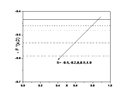
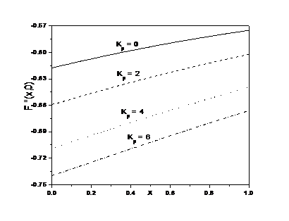
Figures 2(a) – 2(c) represent the fluctuation of skin-friction against x for distinct values of λ, S and KP, respectively. It is obvious from these figures that the skin-friction escalates with the slipperiness and falls down with the fluid suction. Further, it is noticed that the non-similar variable has no effect on the skin-friction coefficient in the presence of velocity slip and fluid suction/injection as shown in the Figures 2(a) and 2(b). In the presence of the porosity parameter KP, the skin-friction reduces and increases with an increase in x as depicted in the Figure 2(c). The effect of the other parameters on the velocity and skin-friction are not much significant and hence graphs are not included.
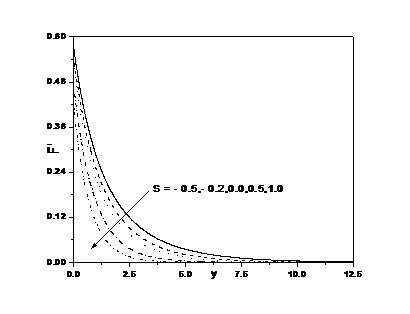
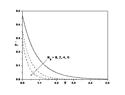
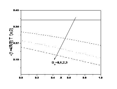
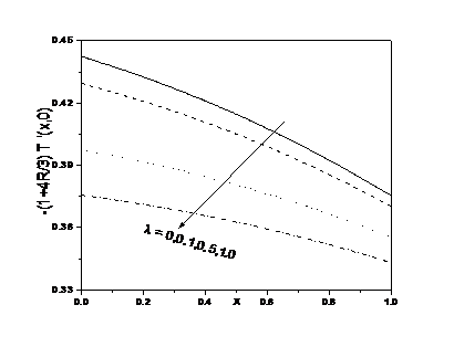
Figures 3(a) – 3(e) exhibit the behaviour of the temperature for different values of Dγ, R, Bi, λ and KP. The temperature rises with an increase in the value of Dγ as shown in the Figure 3(a). It is seen from the Figure 3(b) that the temperature increases with the increasing values of thermal radiation, which in turn, intensifies the thermal boundary layer thickness. Figure 3(c) illustrates that the temperature is enhancing with the rise in the value of Bi and hence gain in the thickness of thermal boundary. Further, for large value of Biot number Bi, the convective thermal condition from (11) transforms to T(0) $\to 1,$ which signifies the constant wall condition. Due to slipperiness, thermal boundary intensifies, and hence, the temperature escalates with an increase in the value of λ as portrayed in the Figure 3(d). Further, Figure 3(e) explores that the temperature increases with an increase in the value of porosity parameter KP.
(a)
(b)
(c)
Figure 2. Effect of (a) λ, (b) S and (c) KP on F"(x,0)
The influence of Dγ, R, Bi, λ and KP on the rate of heat transfer against non-similar variable x is explored in the Figures 4(a) – 4(e). It is evident from the Figure 4(a), that the rate of heat transfer is decreasing with an increase in the value of Dγ. In the absence of Dγ, i.e., Dγ = 0, there is no effect of the non-similar variable x on the rate of heat transfer. As expected, enhancing the value of Dγ, the rate of heat transfer reduces. While the rate of heat transfer escalates with an increase in the value of thermal radiation parameter R as depicted in the Figure 4(b). Figure 4(c) narrates the behaviour of the rate of heat transfer for different values of Biot number Bi. As Biot number enhances, the rate of heat transfer escalates predominantly on the surface due to the strong convection. Figures 4(d) and 4(e) show that the rate of heat transfer reduces with an increase in the values of velocity slip and porosity parameters.
(a)
(b)
(c)
(d)
(e)
Figure 3. Effect of (a) Dγ, (b) R, (c) Bi, (d) λ and (e) KP on T
(a)
(b)
(c)
(d)
(e)
Figure 4. Effect of (a) Dγ, (b) R, (c) Bi, (d) λ and (e) KP on (1+4R/3)T'(x,0)
(a)
(b)
(c)
Figure 5. Effect of(a) Dχ, (b) λ and (c) KP on C
(a)
(b)
(c)
Figure 6. Effect of(a) Dχ, (b) λ and (c) KP on -C'(x,0)
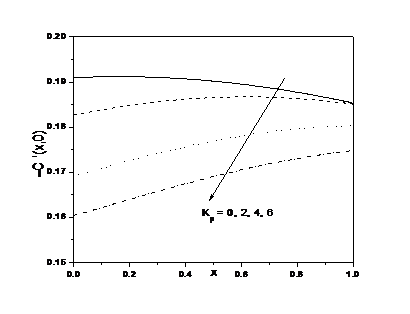
The variation of concentration profile for distinct values of Dχ, λ and KP is shown in the Figures 5(a) – 5(c). An enhancement in the value of Dχ increases the concentration of the fluid as shown in the Figure 5(a). It is noticed from the Figures 5(b) and 5(c) that, as the value of the slip parameter and the porosity parameter increases, the concentration of the fluid increases. Hence, mass transfer at the sheet decreases.
Figures 6(a) – 6(c) depict the behaviour of the rate of mass transfer for different values of Dχ, λ and KP against the non-similar variable x. Enhancing the solute dispersion parameter Dχ, the rate of mass transfer from the sheet to the fluid is falling down. In the absence of Dχ, i.e., Dχ = 0, there is no effect of the non-similar variable x on the rate of mass transfer. As the value of Dχ escalates, the rate of mass transfer reduces as shown in the Figure 6(a). Figures 6(b) and 6(c), it is identified that the rate of mass transfer at the sheet reduces with an increase in the values of velocity slip and porosity parameters. Further, it is identified that in the presence of porosity parameter KP the rate of mass transfer increases gradually as x $\to 1$ .
Numerical investigation of the influence of thermal and solutal dispersions in the presence of thermal radiation on the laminar slip flow, heat and mass transfer of an incompressible viscous fluid over a porous sheet stretching exponentially is analyzed.
[1] Sakiadis BC. (1961). Boundary-layer equations for two-dimensional and axisymmetric flow. A.I.Ch.E. Journal 7(1): 26-28.
[2] Sakiadis BC. (1961). The boundary layer on a continuous flat surface. A.I.Ch.E. Journal 7(2): 221-225.
[3] Pramanik S. (2014). Casson fluid flow and heat transfer past an exponentially porous stretching surface in presence of thermal radiation. Ain Shams Engineering Journal 5(1): 205-212. https://doi.org/10.1016/j.asej.2013.05.003
[4] Khan Y, Smarda Z, Faraz N. (2015). On the study of viscous fluid due to exponentially shrinking sheet in the presence of thermal radiation. Thermal Science 19(1): 191-196.
[5] Remus DE, Marinca V. (2015). Approximate solutions for steady boundary layer MHD viscous flow and radiative heat transfer over an exponentially porous stretching sheet. Applied Mathematics and Computation 269: 389-401. https://doi.org/10.1016/j.amc.2015.07.038
[6] Krupalakshmi KL, Gireesha BJ, Mahanthesh B, Gorla RSR. (2016). Influence of nonlinear thermal radiation and Magnetic field on upper-convected Maxwell fluid flow due to a convectively heated stretching sheet in the presence of dust particles. Communications in Numerical Analysis 2016(1): 57-73. https://doi.org/10.5899/2016/cna-00254
[7] Khan M, Malik MY, Salahuddin T. (2017). Heat generation and solar radiation effects on Carreau nanofluid over a stretching sheet with variable thickness: Using coefficients improved by Cash and Carp. Results in Physics 7: 2512-2519. https://doi.org/10.1016/j.rinp.2017.06.048
[8] Mabood F, Khan WA, Ismail AIMD. (2017). MHD flow over exponential radiating stretching sheet using homotopy analysis method. Journal of King Saud University-Engineering Sciences 29: 68-74. https://doi.org/10.1016/j.jksues.2014.06.001
[9] Thirupathi T, Beg OA, Kadir A. (2017). Numerical study of heat source/sink effects on dissipative magnetic nanofluid flow from a non-linear inclined stretching/shrinking sheet. Journal of Molecular Liquids 232: 159-173. https://doi.org/10.1016/j.molliq.2017.02.032
[10] Naiver CLM. (1827). Sur les lois du mouvement des uides. Memoires del Academie Royale des Sciences. 6: 389-440.
[11] Ullah I, Shafie S, Khan I. (2017). Effects of slip condition and Newtonian heating on MHD flow of Casson fluid over a nonlinearly stretching sheet saturated in a porous medium. Journal of King Saud University–Science 29: 250-259. https://doi.org/10.1016/j.jksus.2016.05.003
[12] Hayat T, Shafiq A, Alsaedi A, Shahzad SA. (2016). Unsteady MHD flow over exponentially stretching sheet with slip conditions. Applied Mathematics and Mechanics 37(2): 193-208. https://doi.org/10.1007/s10483-016-2024-8
[13] Merkin JH. (1994). Natural-convection boundary-layer flow on a vertical surface with Newtonian heating. International Journal of Heat and Fluid Flow 15(5): 392-398. https://doi.org/10.1016/0142-727X(94)90053-1
[14] Hayat T, Imtiaz M, Alsaedi A, Mansoora R. (2014). MHD flow of nanofluids over an exponentially stretching sheet in a porous medium with convective boundary conditions. Chinese Physics B 23(5): 054701. http://stacks.iop.org/1674-1056/23/i=5/a=054701
[15] Rahman M, Rosca AV, Pop I. (2015). Boundary layer flow of a nanofluid past a permeable exponentially shrinking surface with convective boundary condition using Buongiorno’s model. International Journal of Numerical Methods for Heat & Fluid Flow 25(2): 299-319. https://doi.org/10.1108/HFF-12-2013-0361
[16] Khan JA, Mustafa M, Hayat T, Alsaedi A. (2015). Numerical study on three-dimensional flow of nanofluid past a convectively heated exponentially stretching sheet. Canadian Journal of Physics 93(10): 1131-1137. https://doi.org/10.1139/cjp-2014-0433
[17] Mustafa M, Wasim M, Hayat T, Alsaedi A. (2017). A revised model to study the rotating flow of nanofluid over an exponentially deforming sheet: Numerical solutions. Journal of Molecular Liquids 225: 320–327. https://doi.org/10.1016/j.molliq.2016.11.078
[18] Srinivasacharya D, Jagadeeshwar P. (2017). Slip viscous flow over an exponentially stretching porous sheet with thermal convective boundary conditions. International Journal of Applied and Computational Mathematics 3(4): 3525-3537. https://doi.org/10.1007/s40819-017-0311-y
[19] Sparrow EM, Cess RD. (1978). Radiation Heat Transfer Series in Thermal and Fluids Engineering. Augmented ed. 1, McGraw-Hill.
[20] Minkowycz WJ, Sparrow EM. (1974). Local Nonsimilar solutions for natural convection on a vertical cylinder. J. Heat Transfer 96(2): 178-183. https://doi.org/10.111 5/1.3450161
[21] Awad FG, Sibanda P, Motsa SS, Makinde OD. (2011). Convection from an inverted cone in a porous medium with cross-diffusion effects. Computers and Mathematics with Applications 61: 1431-1441. https://doi.org/10.1016/j.camwa.2011.01.015
[22] Canuto C, Hussaini MY, Quarteroni A, Zang TA. (2007). Spectral methods-fundamentals in single domains. Journal of Applied Mathematics and Mechanics 87(1).
[23] Magyari E, Keller B. (1999). Heat and mass transfer in the boundary layers on an exponentially stretching continuous surface. Journal of Physics D: Applied Physics 32: 577-585. http://stacks.iop.org/0022-3727/32/i=5/a=012