Limin Cui | Yonglong Liao*
OPEN ACCESS
This paper puts forward a servomechanism design method for type one discrete-time linear delay system with previewable external interference. The tracking problem was transformed into a regulation problem by setting up an augmented error system, and the input delay was eliminated by a variable substitution. Based on preview control theory and the predictor method, a predictor-preview controller was derived to realize delay compensation and interference preview compensation. Meanwhile, the existence condition of preview controller was given. The effectiveness of the proposed controller was demonstrated through numerical simulation.
discrete-time system, input delay, predictor-preview control, external interference
Preview control fully utilizes the future information of the reference or interference signal, enabling the controller to achieve satisfactory performance. This control strategy has been applied in numerous control systems. One of the earliest applications is the design of a state feedback controller with preview compensation [1]. Later, Katayama et al. [2, 3] studied the preview control in discrete-time and continuous-time systems, drawing on the theory on quadratic optimal regulation, and then designed servomechanisms capable of integral error tracking and preview compensation. Inspired by preview control theory, Liao et al. [4-6] revamped the control mode of multirate sampled-data (MRSD) systems, descriptor systems, and stochastic systems, and put forward a novel design method for augmented system. In engineering, preview control has been widely adopted to enhance motorcycle performance [10, 11], robot walking ability [7-9] and seismic resistance [12].
In recent years, more and more scholars have employed various control strategies to eliminate time delay, a commonplace in practical systems, aiming to ensure the control effect and protect system stability [13-22]. For instance, Reference [23] relies on discrete lifting technique to transform the delay system into a system without delay. Reference [22] proposes a predictive method for discrete-time systems, and, on this basis, designs a preview controller for discrete-time systems with input delay. Reference [24] creates a preview controller through a lifting-predictor method, applies the controller in discrete-time linear systems with state delay and input delay, and effectively reduces the dimension of the augmented system. Reference [25] explores the preview control of discrete-time linear systems with multiple input delays, and provides a controller that supports delay compensation and preview compensation.
Most of the existing studies on the preview control of time delay systems in which the reference signal is previewable. However, there is no report on the design of preview controller for the situation that interference signal is previewable. To make up for this gap, this paper attempts to design a controller capable of preview compensation of interference. Specifically, an augmented error system was established, a variable substitution was given, and then a predictor-preview controller was obtained, which supports both delay compensation and preview compensation of interference.
The remainder of this paper is organized as follows: Section 2 describes the research problem and puts forward basic assumptions; Section 3 constructs an augmented error system by preview control method; Section 4 sets up a predictor-preview controller for the system and provides a numerical example; Section 5 draws a brief conclusion.
A discrete-time system with input delay and external interference can be expressed as:
$\left\{ \begin{align} & x(k+1)=Ax(k)+Bu(k-f)+Ew(k) \\ & y(k)=Cx(k) \\\end{align} \right.$ (1)
where $x(k)\in {{R}^{n}}$ is the state vector; $u(k)\in {{R}^{r}}$ is the input vector; $y(k)\in {{R}^{p}}$ is the output vector; $w(k)\in {{R}^{q}}$ is the external interference; f is a positive integer representing the constant input delay of the system; $A\in {{R}^{n\times n}}$, $B\in {{R}^{n\times r}}$, $C\in {{R}^{p\times n}}$ and $E\in {{R}^{n\times q}}$ are constant matrices; $u(\tau )$ ($\tau =-f,-f+1,\cdots ,0$) are initial inputs; $x(0)={{x}_{0}}$ is the initial state.
The following assumptions were put forward for the said system:
Assumption 1 (A1): The pair $(A,B)$ is stabilizable, $(C,A)$ is detectable, and the matrix $\left[ \begin{matrix} A & B \\ C & 0 \\\end{matrix} \right]$ is of full row rank.
Assumption 2 (A2): The external interference $w(k)$ is previewable, with the preview length of ${{N}_{w}}$. In other words, at the current execution time k, the value $w(k)$ and the ${{N}_{w}}$ future values $w(k+1)$, … , $w(k+N_w)$ are available. The future values of the interference signal beyond time $w(k+N_w)$ can be approximated by $w(k+N_w)$, i.e. $w(k+l)=w(k+{{N}_{w}})$ ($l\ge {{N}_{w}}+1$).
Let $r(k)\in {{R}^{p}}$ be the reference signal satisfying
$\underset{k\to \infty }{\mathop{\lim }}\,r(k)=\bar{r}$
where $\bar{r}$ is a constant vector. This means $r(k)$ reaches a steady state.
Furthermore, it is assumed that $e(k)$ is the error signal defined as the difference between $y(k)$ and $r(k)$:
$e(k)=y(k)-r(k)$
Then, our research aims to design a controller capable of preview compensation of interference , such that the output $y(k)$ of the closed-loop system of (1) tracks the reference signal $r(k)$:
$\underset{k\to \infty }{\mathop{\lim }}\,e(k)=0$.
For convenience, the quadratic performance index of (1) can be described as [22]:
$J=\sum\limits_{k=1}^{\infty }{\left[ {{e}^{T}}(k){{Q}_{e}}e(k)+\Delta {{u}^{T}}(k-f)H\Delta u(k-f) \right]}$ (2)
where ${{Q}_{e}}\in {{R}^{p\times p}}$ and $H\in {{R}^{r\times r}}$ are positive definite weight matrices; $\Delta$ is the first-order backward difference operator satisfying $\Delta u(k)=u(k)-u(k-1)$.
The preview controller for (1) was designed in three steps: setting up an augmented error system, deriving a controller from this system, and acquiring the controller for the original system.
Finding the first-order backward differences on both sides of (1), we have:
$\Delta x(k+1)=A\Delta x(k)+B\Delta u(k-f)+E\Delta w(k)$ (3)
If $e(k+1)=Cx(k+1)-r(k+1)$, the following equation can be derived through first-order backward difference operation:
$\Delta e(k+1)=C\Delta x(k+1)-\Delta r(k+1)$. (4)
Since $\Delta e(k+1)=e(k+1)-e(k)$, the error signal satisfies:
$\begin{align} & e(k+1)=e(k)+CA\Delta x(k)+ \\ & CB\Delta u(k-f)+CE\Delta w(k)-\Delta r(k+1) \\\end{align}$ (5)
where the dynamic equation (3) is used.
Future reference signal is not used to design the controller, which only supports preview compensation of interference. Hence, reference signal $r(k+l)$ ($l=1,2,\cdots $) can be viewed as a constant at current execution time k. Thus, $\Delta r(k+1)=0$ and (5) can be rewritten as:
$e(k+1)=e(k)+CA\Delta x(k)+CB\Delta u(k-f)+CE\Delta w(k)$ (6)
Combining (3) and (6), we have:
$\left\{ \begin{align} & X(k+1)=\bar{A}X(k)+\bar{B}\Delta u(k-f)+\bar{E}\Delta w(k) \\ & e(k)=\bar{C}X(k) \\ \end{align} \right.$ (7)
where $X(k)=\left[ \begin{matrix} e(k) \\ \Delta x(k) \\\end{matrix} \right]$; $\bar{A}=\left[ \begin{matrix} {{I}_{p}} & CA \\ 0 & A \\\end{matrix} \right]$; $\bar{B}=\left[ \begin{matrix} CB \\ B \\\end{matrix} \right]$; $\bar{C}=\left[ \begin{matrix} {{I}_{p}} & 0 \\\end{matrix} \right]$; $\bar{E}=\left[ \begin{matrix} CE \\ E \\\end{matrix} \right]$.
Equation (7) is the augmented error system of (1). Since $y(k)$ of (1) is available and $r(k)$ is previewable, it is suitable to take $e(k)=\bar{C}X(k)$ as the output of (7).
Correspondingly, the performance index (2) can be expressed as:
$J=\sum\limits_{k=1}^{\infty }{\left[ {{X}^{T}}(k)QX(k)+\Delta {{u}^{T}}(k-f)H\Delta u(k-f) \right]}$ (8)
where $Q=\left[ \begin{matrix} {{Q}_{e}} & {{0}_{{}}} \\ {{0}_{{}}} & {{0}_{{}}} \\\end{matrix} \right]$.
The next task is to design a controller $\Delta u(k)$ subjected to dynamic constraint (7) such that the performance index (8) reaches minimum. It is easy to learn that $\underset{k\to \infty }{\mathop{\lim }}\,X(k)=0$. Obviously, the conclusion $\underset{k\to \infty }{\mathop{\lim }}\,e(k)=0$ is valid. Besides, the input $u(k)$ can be derived from $\Delta u(k)$.
Let us introduce a new input vector
$v(k)=\Delta u(k-f)$ (9)
Substituting (9) into (7) and (8) respectively, we have:
$\left\{ \begin{align} & X(k+1)=\bar{A}X(k)+\bar{B}v(k)+\bar{E}\Delta w(k) \\ & e(k)=\bar{C}X(k) \\ \end{align} \right.$ (10)
and
$J=\sum\limits_{k=1}^{\infty }{\left[ {{X}^{T}}(k)QX(k)+{{v}^{T}}(k)Hv(k) \right]}$ (11)
The augmented system (10) is without any delay. It can be seen from A2 that the interference signal $w(k)$ is previewable in the sense that the future value $\Delta w(l)\text{ }(k\le l\le k+{{N}_{w}})$ is available at each execution time k. The following theorem will stand based on the results of Reference [26]:
Theorem 1. If A1 and A2 hold and ${{Q}_{e}}$ is positive definite, then the controller with interference preview compensation of (10) that minimizes criterion (11) can be described as:
$v(k)=-{{G}_{X}}X(k)-\sum\limits_{l=0}^{{{N}_{w}}}{{{G}_{w}}(l)\Delta w(k+l)}$ (12)
where ${{G}_{X}}={{\left[ H+{{{\bar{B}}}^{T}}P\bar{B} \right]}^{-1}}{{\bar{B}}^{T}}P\bar{A}$;
${{G}_{w}}(l)={{\left[ H+{{{\bar{B}}}^{T}}P\bar{B} \right]}^{-1}}{{\bar{B}}^{T}}{{({{\bar{A}}_{c}}^{T})}^{l}}P\bar{E}$, $l=0,1,\cdots ,{{N}_{w}}$.
Note that $P\in {{R}^{(p+n)\times (p+n)}}$ is the positive semi-definite solution of the algebraic Riccati equation:
$P={{\bar{A}}^{T}}P\bar{A}-{{\bar{A}}^{T}}P\bar{B}{{\left[ H+{{{\bar{B}}}^{T}}P\bar{B} \right]}^{-1}}{{\bar{B}}^{T}}P\bar{A}+Q$.
${{\bar{A}}_{c}}$ is the closed-loop matrix:
${{\bar{A}}_{c}}=\bar{A}-\bar{B}{{\left[ H+{{{\bar{B}}}^{T}}P\bar{B} \right]}^{-1}}{{\bar{B}}^{T}}P\bar{A}$
Remark 1: The value of future interference signal $\Delta w(k+l)$ ($l=1,\cdots ,{{N}_{w}}$) in $-\sum\limits_{l=0}^{{{N}_{w}}}{{{G}_{w}}(l)\Delta w(k+l)}$ acts as a preview compensation in the controller.
The preview controller for the augmented error system (7) can be derived from Theorem 1 as follows.
Combining (9) and (12), we have:
$\Delta u(k-f)=-{{G}_{X}}X(k)-\sum\limits_{l=0}^{{{N}_{w}}}{{{G}_{w}}(l)\Delta w(k+l)}$
Replacing k-f by k, we have:
$\Delta u(k)=-{{G}_{X}}X(k+f)-\sum\limits_{l=0}^{{{N}_{w}}}{{{G}_{w}}(l)\Delta w(k+f+l)}$ (13)
where the current control input $\Delta u(k)$ uses the future state vector $X(k+f)$. The latter should be predicted to ensure the executability of the controller. Through stepwise iteration, the dynamic equation of (7) can be solved as:
$X(k+1)=\bar{A}X(k)+\bar{B}\Delta u(k-f)+\bar{E}\Delta w(k)$
In this way, the future value of the state vector can be derived as:
$\begin{align} & X(k+f)={{{\bar{A}}}^{f}}X(k)+\sum\limits_{l=0}^{f-1}{{{{\bar{A}}}^{(f-1-l)}}\bar{B}\Delta u(k+l-f)} \\ & +\sum\limits_{l=0}^{f-1}{{{{\bar{A}}}^{(f-1-l)}}\bar{E}\Delta w(k+l)} \\\end{align}$ (14)
The future value $X(k+f)$ can be predicted by (14). According to A2, for the preview length ${{N}_{w}}\ge f$, the vectors $\Delta w(k+l)$ are available at $l=0,1,\cdots ,f$; for the preview length ${{N}_{r}}<f$, the vectors $\Delta w(k+l)$ are available at $l=0,1,\cdots ,{{N}_{r}}$, and $\Delta w(k+l)=0$ at $l={{N}_{r}}+1,\cdots ,f$. The analysis shows that all the values in (14) are available. Equation (14) shows that the future state vector X(k+f) is determined by the current state vector X(k), the past control input $\Delta u(k+l-f)$ ($l=0,\cdots ,f-1$), and the difference $\Delta w(k+l)$ ($l=0,\cdots ,f-1$) of the future interference signal. The predictor method used above is a generalization of the predictor feedback method [22, 25].
Substituting (14) into (13), the feedback control law of the augmented error system (7) can be obtained as:
$\begin{align} & \Delta u(k)=-{{G}_{X}}{{{\bar{A}}}^{f}}X(k)-{{G}_{X}}\sum\limits_{l=0}^{f-1}{{{{\bar{A}}}^{(f-1-l)}}\bar{B}\Delta u(k+l-f)} \\ & -{{G}_{X}}\sum\limits_{l=0}^{f-1}{{{{\bar{A}}}^{(f-1-l)}}\bar{E}\Delta w(k+l)}-\sum\limits_{l=0}^{{{N}_{w}}}{{{G}_{w}}(l)\Delta w(k+f+l)} \\ \end{align}$ (15)
For the last term $-\sum\limits_{l=0}^{{{N}_{w}}}{{{G}_{w}}(l)\Delta w(k+f+l)}$, if $k+f+l>k+{{N}_{w}}$, then $\Delta w(k+f+l)=0$. It is obvious that (15) is an executable controller of (7) for all parts in (15) are available.
To derive a preview controller for (1), it is firstly assumed that
${{G}_{X}}{{\bar{A}}^{f}}=\left[ \begin{matrix} {{G}_{e}} & {{G}_{x}} \\\end{matrix} \right]$ (16)
where ${{G}_{e}}\in {{R}^{r\times p}}$ and ${{G}_{x}}\in {{R}^{r\times n}}$. Then, (15) can be rewritten as:
$\begin{align} & \Delta u(k)=-{{G}_{e}}e(k)-{{G}_{x}}\Delta x(k)-{{G}_{X}}\sum\limits_{l=0}^{f-1}{{{{\bar{A}}}^{(f-1-l)}}\bar{B}\Delta u(k+l-f)} \\ & -{{G}_{X}}\sum\limits_{l=0}^{f-1}{{{{\bar{A}}}^{(f-1-l)}}\bar{E}\Delta w(k+l)}-\sum\limits_{l=0}^{{{N}_{w}}}{{{G}_{w}}(l)\Delta w(k+f+l)} \\ \end{align}$ (17)
The initial values of system (1) and the reference signal are assumed as zeros, that is, for $k=-f,-f+1,\cdots ,0$, the vectors x(k)=0, y(k)= r(k)=0, u(k)=0 and w(k)=0. Then, it is easy to infer from (17) that:
$\begin{align} & u(k)=-{{G}_{e}}\sum\limits_{j=1}^{k}{e(j)}-{{G}_{x}}x(k)-{{G}_{X}}\sum\limits_{l=0}^{f-1}{{{{\bar{A}}}^{(f-1-l)}}\bar{B}u(k+l-f)} \\ & -{{G}_{X}}\sum\limits_{l=0}^{f-1}{{{{\bar{A}}}^{(f-1-l)}}\bar{E}w(k+l)}-\sum\limits_{l=0}^{{{N}_{w}}}{{{G}_{w}}(l)w(k+f+l)} \\\end{align}$
Thus, the preview control theory for system (1) can be established as follows.
Theorem 2. If A1 and A2 hold, Qe is positive definite, and the performance index is defined as (3), then the preview controller of (1) can be described as (18), provided that x(k)=0, y(k)= r(k)=0, u(k)=0, w(k)=0 for $k=-f,-f+1,\cdots ,0$.
$u(k)=-{{G}_{e}}\sum\limits_{j=1}^{k}{e(j)}-{{G}_{x}}x(k)-{{f}_{1}}(k)-{{f}_{2}}(k)$ (18)
where ${{f}_{1}}(k)={{G}_{X}}\sum\limits_{l=0}^{f-1}{{{{\bar{A}}}^{(f-1-l)}}\bar{B}u(k+l-f)}$;
$\begin{align} & {{f}_{2}}(k)={{G}_{X}}\sum\limits_{l=0}^{f-1}{{{{\bar{A}}}^{(f-1-l)}}\bar{E}w(k+l)}+ \\ & \sum\limits_{l=0}^{{{N}_{w}}}{{{G}_{w}}(l)w(k+f+l)} \\\end{align}$.
The matrices Ge and Qx are determined by (16), GX and Gw are given by Theorem 1.
Remark 2: According to A2, at each execution time k, for the general term $w(k+f+l)$ in $\sum\limits_{l=0}^{{{N}_{w}}}{{{G}_{w}}(l)w(k+f+l)}$, if $f+l\le {{N}_{w}}$, then the real value of $w(k+f+l)$ is taken; if $f+l>{{N}_{w}}$, then $w(k+f+l)=w(k+{{N}_{w}})$ is taken.
Remark 3: For the four terms of the preview controller (18), the first term $-{{G}_{e}}\sum\limits_{j=1}^{k}{e(j)}$ is the cumulative tracking error used to eliminate the static error; the second term $-{{G}_{x}}x(k)$ is the state feedback; the third term $-{{f}_{1}}(k)$ is the compensation of the input delay; the last term $-{{f}_{2}}(k)$ is the preview compensation of the interference signal. The design process indicates that the interference signal is also used to compensate for the input delay.
Next, the validity of the proposed controller was verified through numerical simulation.
Example 1. For control system (1), it is assumed that $A=\left[ \begin{matrix} 1 & 1 \\ 0 & 1 \\\end{matrix} \right]$, $B=\left[ \begin{matrix} 0 \\ 0.01 \\\end{matrix} \right]$, $C=\left[ \begin{matrix} 1 & 2 \\\end{matrix} \right]$ and $E=\left[ \begin{matrix} 0 \\ -0.5 \\\end{matrix} \right]$. Three delays f=10, f=20 and f=30 were simulated. The reference signal r(t) and interference signal w(t) were respectively set up as:
$r(k)=\left\{ \begin{align} & 0,\text{ }k<20 \\ & 1,\text{ }k\ge 20 \\ \end{align} \right.$
$w(k)=\left\{ \begin{align} & 0,\text{ }k<30 \\ & 0.2,\text{ }k\ge 30 \\ \end{align} \right.$
The verification results show that the pair (A,B) was stabilizable, (C,A) was detectable, and the matrix $\left[ \begin{matrix} A & B \\ C & 0 \\\end{matrix} \right]$ was of full row rank. These fully satisfy Assumption A1. Let the weight matrices Qe=1.0 and H=0.04. By Theorem 2, there exists a preview controller described as (18) for control system (1). The output responses with and without preview compensation were illustrated in Figure 1 below.
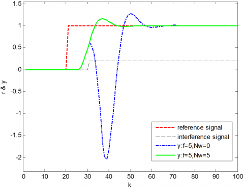
Figure 1. The output responses with and without preview compensation
As shown in Figure 1, the interference had a greater impact on the closed-loop system when the controller cannot perform preview compensation. This means the preview compensation can effectively reduce the impact of interference.
Figure 2 presents the output responses of the closed-loop system with different delays when the preview length of the interference signal is Nw=5.
Figure 2. The output responses with different delays
Figure 2 shows that, under the same preview length, the tracking of output response to the reference signal worsened with the increase in the delay. Thus, the interference preview compensation of the controller can compensate for both external interference and time delay.
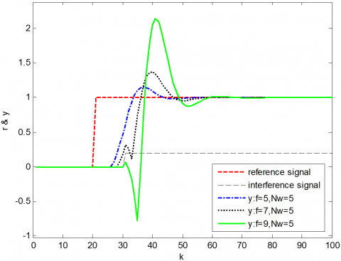
Figure 3 displays the output responses of the closed-loop system with the input delay f=5 at different preview lengths (Nw=5, Nw=7, and Nw=9).
Figure 3. The output responses with different preview lengths
It can be seen that the future value of the reference signal was only used to compensate for the delay, when the preview length was equal to the input delay. The preview length should be increased to improve the performance. Once the preview length reached Nw=9, the tracking error was greatly reduced and the response was improved efficiently.
The proposed controller supports the preview compensation of interference signal, but not reference signal. As a result, the output of the closed-loop system only responds to the change of the interference signal in advance, without responding to that of the reference signal in advance.
This paper tackles the design of type one preview controller for discrete-time linear systems with input delay, and successfully derives a preview controller that compensates for both input delay and interference in advance. The input delay was overcome by predictor feedback. The proposed controller was proved effective through numerical simulation. The future research will probe into another complex but significant problem: selecting a proper preview length according to the features of interference signal and time delay system.
The authors would like to thank Beijing Municipal Education Commission Scientific Research Plan, Social Science Plan General Project for their financial support under the grant number of No. KM201710017004, and the Project of “Passing the Scientific Research” for the Young Teachers of Beijing Institute of Petrochemical Technology.
[1] Hayase M, Ichikawa K. (1969). Optimal servosystem utilizing future value of desired function. Transactions of Society of Instrument and Control Engineers 5(1): 86-94. https://doi.org/10.9746/sicetr1965.5.86
[2] Katayama T, Ohki T, Inoue T, Kato T. (1985). Design of an optimal controller for a discrete-time system subject to previewable demand. International Journal of Control 41(3): 677-699. https://doi.org/10.1080/0020718508961156
[3] Katayama T, Hirono T. (1987). Design of an optimal servomechanism with preview action and its dual problem. International Journal of Control 45(2): 407-420. https://doi.org/10.1080/00207178708933740
[4] Liao F, Takaba K, Katayama T, Katsuura J. (2003). Design of an optimal preview servomechanism for discrete-time systems in multirate setting. Dynamics of Continuous, Discrete, and Impulsive Systems Series B: Applications and Algorithms, 10(5): 727-744. https://doi.org/10.1215/S0012-7094-03-12017-7
[5] Liao F, Cao M, Hu Z, An P. (2012). Design of an optimal preview controller for linear discrete-time causal descriptor systems. International Journal of Control 85(10): 1616-1624. https://doi.org/10.1080/00207179.2012.695804
[6] Wu J, Liao F, Tomizuka M. (2017). Optimal preview control for a linear continuous-time stochastic control system in finite-time horizon. International Journal of Systems Science 48(1): 129-137. ttps://doi.org/10.1080/00207721.2016.1160456
[7] Sharp RS. (2007). Optimal preview speed-tracking control for motorcycles. Multibody System Dynamics 18: 397-411. https://doi.org/10.1007/s11044-007-9079-x
[8] Marzbanrad J, Hojjat Y, Zohoor H, Nikravesh SK. (2003). Optimal preview control design of an active suspension based on a full car model. Scientia Iranica 10(1): 23-36.
[9] Kajita S, Kanehiro F, Kaneko K, Fujiwara K, Harada K, Yokoi K, Hirukawa H. (2003). Biped walking pattern generation by using preview control of zero-moment point. Proceedings of the 2003 IEEE International Conference on Robotics and Automation, Taipei, Taiwan, September (2): 1620-1626. https://doi.org/10.1109/ROBOT.2003.1241826
[10] Shimmyo S, Sato T, Ohnishi K. (2013). Biped walking pattern generation by using preview control based on three-mass model. IEEE Transactions on Industrial Electronics 60(11): 5137-5147. https://doi.org/10.1109/tie.2012.2221111
[11] Czarnetzki S, Kerner S, Urbann O. (2009). Observer-based dynamic walking control for biped robots. Robotics and Autonomous Systems 57(8): 839-845. https://doi.org/10.1016/j.robot.2009.03.007
[12] Marzbanrad J, Ahmadi G, Jha R. (2004). Optimal preview active control of structures during earthquakes. Engineering Structures 26(10): 1463-1471. https://doi.org/10.1016/j.engstruct.2004.05.010
[13] Fridman E. (2014). Introduction to Time-Delay Systems: Analysis and Control, Birkhauser.
[14] Smith OJM. (1959). A controller to overcome dead time. Journal of Instrument Society of America 6(2): 28-33.
[15] Furukawa T, Shimemura E. (1983). Predictive control for systems with time delay. International Journal of Control 37(2): 399-412. https://doi.org/10.1080/00207178308932979
[16] Manitius AZ, Olbrot AW. (1979). Finite spectrum assignment problem for systems with delays. IEEE Transactions on Automatic Control 24(4): 541-553. https://doi.org/10.1109/tac.1979.1102124
[17] Mondié S, Michiels W. (2003). Finite spectrum assignment of unstable time-delay systems with a safe implementation. IEEE Transactions on Automatic Control 48(12): 2207-2212. https://doi.org/10.1109/tac.2003.820147
[18] Michiels W, Mondié S, Roose D, Dambrine M. (2004). The effect of approximating distributed delay control laws on stability. Advances in Time-Delay Systems: Lecture Notes in Computer Science and Engineering. Berlin, Germany: Springer (38): 207-222. https://doi.org/10.1007/978-3-642-18482-6_15
[19] Kharitonov VL. (2015). Predictor-based controls: the implementation problem. Differential Equations 51(13): 1675-1682. https://doi.org/10.1134/S0012266115130017
[20] Molnar TG, Insperger T. (2016). On the robust stabilizability of unstable systems with feedback delay by finite spectrum assignment. Journal of Vibration and Control 22(3): 649-661. https://doi.org/10.1177/1077546314529602
[21] Liao Y, Liao F. (2018). Design of preview controller for linear continuous-time systems with input delay. International Journal of Control, Automation and Systems 16(3): 1080-1090. https://doi.org/10.1007/s12555-016-0209-1
[22] Liao F, Liao Y, Deng J. (2016). The application of predictor feedback in designing a preview controller for discrete-time systems with input delay. Mathematical Problems in Engineering. http://dx.doi.org/10.1155/2016/3023915
[23] Cao M, Liao F. (2015). Design of an optimal preview controller for linear discrete-time descriptor systems with state delay. International Journal of Systems Science 46(5): 932-943. https://doi.org/10.1155/2017/1414029
[24] Liao Y, Liao F. (2017). Design of preview controller for discrete-time linear systems with time delay by using the lifting-predictor method. Control and Decision 32(8): 1359-1367. https://doi.org/10.13195/j.kzyjc.2016.0672
[25] Cui L, Liao Y, Zheng D. (2018). A design method of preview controller for discrete-time systems with multiple input delays. Journal Europeen des Systemes Automatises 51(1-3): 75-87. https://doi.org/10.3166/JESA.51.75-87
[26] Tsuchiya T, Egami T. (1994). Digital preview and predictive control. Beijing: Beijing Science and Technology Press 34-56.