Améni Driss | Samah Maalej | Isra Chouat | Mohamed Chaker Zaghdoudi*
OPEN ACCESS
An experimental study is carried out in order to determine the thermal performances of a water-cooled heat pipe cooling system. An experiment rig is designed, fabricated and fully instrumented to test the cooling system prototype. The results show that the maximum heat transport capacity of the heat pipe increase with the water-cooling temperature; however, its overall thermal resistance decreases. Correlations for heat transfer in the evaporator and condenser sections are proposed. A model is also developed in order to determine the capillary limit as well as the heat transfer in the heat pipe. The model can predict the experimental results within -1.7 % and +7.9 % when estimating the capillary limit and underestimates the heat pipe overall thermal resistance within -17.8 % and -9.7 %; however, it overestimates the evaporator temperature within 4.4 % and 9.5 %.
capillary pumping, electronics cooling, heat pipes, grooves
Power conversion modules include semiconductor components that insure the control of the energy transfer. Components such as IGBT enable to increase the frequency of the converter operation. Because of the high commutative power levels and high operating frequencies, and since the power modules tend to become more and more compact, the power densities dissipated from such components are very high, which causes a reduction in their lifetime and could lead to their damage. Hence, it is necessary to use effective cooling systems capable to evacuate the heat generated and maintain the junction temperature of the electronic component at values allowing safe operation.
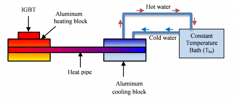
An efficient classic cooling system is composed by cold plates that insure the cooling underneath the IGBT by fluid circulation. This solution presents drawbacks since the electrical operation can fail due to fluid leakage. A solution to this problem is to remove the heat by a heat pipe system placed underneath the IGBT. The heat is rejected by a cold plate, which is cooled by liquid circulation (Figure 1). This solution could be as efficient as the classic one if the heat pipe thermal resistance is very low.
The thermal performances of the heat pipes depend on several parameters among them we can distinguish: (i) the geometrical characteristics, (ii) the operating conditions such as the heat input power, the heat sink temperature, and the external field forces (gravity, accelerations, vibrations, magneto-hydrodynamic, and electrohydrodynamic), (iii) the characteristics of the capillary structures (grooves, sintered powder, screen meshes, metal wires or a mixture of them), and (iv) the working fluid.
The grooved cylindrical heat pipes are commonly used in standard electronics cooling applications because their thermal resistances are lower than those including other capillary structures; however, their thermal performances can be altered when considering special operating conditions, especially including gravity and acceleration.
Previous studies on grooved cylindrical heat pipes have reported thermal performances in either steady state or transient regime [1-13]. Tests on transient state regime have been paid a special attention since it is important to identify the thermal behavior of the heat pipes in these conditions as the electronic components are working in the most of time in transient conditions [9, 10].
Figure 1. Heat pipe-based cooling system
Although the experimental studies dealing with steady-state conditions are numerous; however, they do not propose generalized laws in order to identify the heat transfer in the evaporation and condensation zones. As a generalized correlation is important for the calculation of the evaporator and the condenser thermal resistances that are useful in theoretical models for the prediction of the heat pipe thermal behavior in steady state or transient regimes, this study addresses this issue. Hence, in the first part on this work, an experimental study is carried out to determine the thermal performances of a based-heat pipe cooling system. Since the heat pipe plays an important role in such systems, tests are carried out on a water-filled copper cylindrical heat pipe including helicoidally and trapezoidal capillary grooves. A test rig is developed in order to determine the thermal performance of the heat pipe, which is positioned horizontally, for different heat sink temperatures. In the second part of this study, a theoretical model is developed to determine the capillary limit and the heat transfer within the heat pipe for various operating conditions. Finally, a comparison between the simulated results and those obtained experimentally is realized.
2.1 Description of the heat pipe
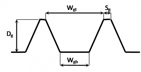
A water-filled cylindrical copper heat pipe is used (Figure 2). The capillary structure is composed of 75 helicoidally and trapezoidal grooves (Figure 3). The main geometrical characteristics of the heat pipe are listed in Table 1.
Figure 2. Cross-section of the heat pipe showing the grooves
Figure 3. Geometrical characteristics of the grooves
Table 1. Geometrical characteristics of the heat pipe
|
Parameters |
Values |
|
Heat Pipe |
|
|
Heat pipe length, Lt |
190 mm |
|
Evaporator length, Lev |
60 mm |
|
Condenser length, Lc |
60 mm |
|
Outer diameter, Do |
15.87 mm |
|
Wall thickness, tw |
0.58 mm |
|
Grooves |
|
|
Number of grooves, Ng |
75 |
|
Groove depth, Dg |
0.3 mm |
|
Groove width at the bottom of the groove, Wgb |
0.266 mm |
|
Groove width at the top of the groove, Wgt |
0.599 mm |
|
Angle between the groove and the heat pipe axis, a (Figure 2) |
20 ° |
|
Angle b (Figure 2) |
29 ° |
2.2 Test rig and experimental procedures
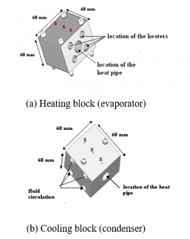
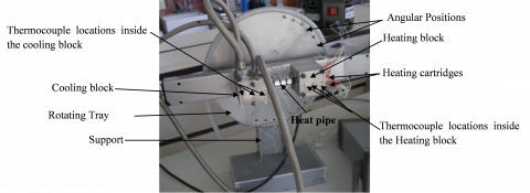
An experimental set-up was built up in order to determine the thermal performance of the cooling system for different positions at various heat input powers, Q, and heat sink temperatures, Ths. It is composed by two aluminum blocks. The first block is equipped with four electrical and cylindrical heaters dissipating 250 W each. This heating block (60 × 60 × 60 mm3) plays the role of the heat source (Figure 4a). The second block (cold plate), which has the same dimensions as the heating block, is cooled by water circulation that is insured by means of a pump (Figure 4b). The temperature of the water at the inlet of the cooling block is controlled by a refrigerated circulation bath. The heating and cooling blocks are mounted on a rotating support in order to study the thermal performances of the system as a function of the orientation (Figure 5). A thermal paste is used to improve the thermal contact between the heat pipe and the aluminum blocks. A HP 34970 data acquisition unit is used in order to monitor and record all the temperatures (Figure 6). Ten T-type thermocouples are placed along the heat pipe in order to measure the temperature distribution and its evolution in time (Figure 7).
Figure 4. Sketches of the heating and cooling blocks
Figure 5. View of the experimental set-up (without thermal insulation)
Figure 6. Test rig arrangement
Figure 7. Thermocouple location along the heat pipe
The experimental procedures consist of positioning the cooling system in the proper orientation. Then, the heat sink temperature is fixed by adjusting the water temperature at the cooling block inlet. Then, the power is adjusted to the desired value and the system can reach the steady-state regime. The temperature readings from all thermocouples are recorded. After the steady-state regime is reached, the power to the evaporator is turned off. This cycle of experiments is repeated with higher input heat powers until the maximum heat power (capillary limit) is reached. This is characterized by a sudden and steady rise of the evaporator temperature.
2.3 Data reduction and uncertainty analysis
The overall thermal resistance of the heat pipe is determined by the following equation
${{R}_{th}}\text{ }=\text{ }{{\text{R}}_{\text{thev}}}\text{ }+\text{ }{{\text{R}}_{\text{thad}}}\text{ }+\text{ }{{\text{R}}_{\text{thc}}}\text{ }=\text{ }{\left( {{{\text{\bar{T}}}}_{\text{ev}}}-{{{\bar{T}}}_{c}} \right)}/{Q}\;=\frac{\Delta {{{\bar{T}}}_{hp}}}{Q}$ (1)
Rthev, Rthad, and Rthc are the thermal resistances of the evaporator, adiabatic and condenser zones, respectively, and Q is the heat input power. ${{\bar{T}}_{ev}}$ and $ {{\bar{T}}_{c}}$ are the average wall temperature of the evaporator and the condenser, respectively. $\Delta {{\bar{T}}_{hp}}$is the temperature difference ${{\bar{T}}_{ev}}- {{\bar{T}}_{c}}$.
The evaporator and condenser thermal resistances are calculated according to
${{R}_{thev}}\text{ }=\text{ }\frac{{{{\text{\bar{T}}}}_{\text{ev}}}-{{{\bar{T}}}_{ad}}}{Q}\text{ }={{\text{R}}_{\text{thwev}}}+{{R}_{thevap}}=\frac{{{t}_{w}}}{{{\lambda }_{w}}\text{ }{{\text{A}}_{\text{ev}}}}+\frac{1}{{{h}_{ev}}\text{ }{{\text{A}}_{\text{ev}}}}$ (2)
${{R}_{thc}}\text{ }=\text{ }\frac{{{{\text{\bar{T}}}}_{\text{ad}}}-{{{\bar{T}}}_{c}}}{Q}\text{ }={{\text{R}}_{\text{thwc}}}+{{R}_{thcond}}=\frac{{{t}_{w}}}{{{\lambda }_{w}}\text{ }{{\text{A}}_{\text{c}}}}+\frac{1}{{{h}_{c}}\text{ }{{\text{A}}_{\text{c}}}}$ (3)
Rthwev and Rthwc are the thermal resistances due to thermal conduction through the evaporator and the condenser walls, respectively. tw and lw are the thickness and the thermal conductivity of the wall, respectively. Aev and Ac are the inner evaporator and condenser areas, respectively. In Eqns. (2) and (3), the conductive thermal resistances of the heat pipe wall are calculated by assuming that the wall thickness is negligible when compared to the heat pipe diameter. Hence, under this assumption, the expression of the thermal resistance for a cylindrical wall is similar to that for a flat one.
From Eqns. (2) and (3), the heat transfer coefficients for the evaporation and condensation phenomena are calculated according to the following expressions
${{h}_{ev}}\text{ }=\text{ }\frac{\text{1}}{\frac{\left( {{{\text{\bar{T}}}}_{\text{ev}}}\text{ - }{{{\text{\bar{T}}}}_{\text{ad}}} \right)}{{{\text{q}}_{\text{ev}}}}-\frac{{{t}_{w}}}{{{\lambda }_{w}}}}=\frac{1}{\frac{\Delta {{{\bar{T}}}_{ev}}}{{{q}_{ev}}}-\frac{{{t}_{w}}}{{{\lambda }_{w}}}}$ (4)
${{h}_{c}}\text{ }=\text{ }\frac{\text{1}}{\frac{\left( {{{\text{\bar{T}}}}_{\text{ad}}}\text{ - }{{{\text{\bar{T}}}}_{\text{c}}} \right)}{{{\text{q}}_{\text{c}}}}-\frac{{{t}_{w}}}{{{\lambda }_{w}}}}=\frac{1}{\frac{\Delta {{{\bar{T}}}_{c}}}{{{q}_{c}}}-\frac{{{t}_{w}}}{{{\lambda }_{w}}}}$ (5)
qev and qc are the heat fluxes calculated on the basis the evaporator and condenser heat transfer areas, Aev and Ac.$\Delta {{\bar{T}}_{ev}}$.and $\Delta {{\bar{T}}_{c}}$ are the temperature differences ${{\bar{T}}_{ev}}- {{\bar{T}}_{ad}}$ and ${{\bar{T}}_{ad}}- {{\bar{T}}_{c}}$, respectively.
The uncertainty for the thermal resistance, URth, is given by the root sum square of the uncertainties of the bias contribution to the uncertainty of Rth, BRth, and the precision contribution to the uncertainty of Rth, PRth, according to [14]
${{U}_{{{R}_{th}}}}={{({{B}^{2}}_{{{R}_{th}}}+{{P}^{2}}_{{{R}_{th}}})}^{1/2}}$ (6)
The precision and bias limits contributions can be determined separately in terms of the sensitivity coefficients of the thermal resistance, Rth, according to the following expressions [14]
$P_{Rth}^{2}={{\left( \frac{\partial {{R}_{th}}}{\partial {{{\bar{T}}}_{ev}}} \right)}^{2}}P_{{{{\bar{T}}}_{ev}}}^{2}+{{\left( \frac{\partial {{R}_{th}}}{\partial {{{\bar{T}}}_{c}}} \right)}^{2}}P_{{{{\bar{T}}}_{c}}}^{2}+{{\left( \frac{\partial {{R}_{th}}}{\partial Q} \right)}^{2}}P_{Q}^{2}$ (7)
$B_{Rth}^{2}={{\left( \frac{\partial {{R}_{th}}}{\partial {{{\bar{T}}}_{ev}}} \right)}^{2}}B_{{{{\bar{T}}}_{ev}}}^{2}+{{\left( \frac{\partial {{R}_{th}}}{\partial {{{\bar{T}}}_{c}}} \right)}^{2}}B_{{{{\bar{T}}}_{c}}}^{2}+{{\left( \frac{\partial {{R}_{th}}}{\partial Q} \right)}^{2}}B_{Q}^{2}+\left( \frac{\partial {{R}_{th}}}{\partial {{{\bar{T}}}_{ev}}} \right)\times \left( \frac{\partial {{R}_{th}}}{\partial {{{\bar{T}}}_{c}}} \right)B_{{{{\bar{T}}}_{ev}}}^{'}B_{{{{\bar{T}}}_{c}}}^{'}$ (8)
where B'Tc and B'Tev are the portions of BTc and BTev, that arise from identical error source and they are therefore presumed to be perfectly correlated.
By considering the expression of Rth, the precision and bias limits contributions can be expressed as
${{\left( \frac{{{P}_{{{R}_{th}}}}}{{{R}_{th}}} \right)}^{2}}={{\left( \frac{{{P}_{{{{\bar{T}}}_{ev}}}}}{\Delta {{{\bar{T}}}_{hp}}} \right)}^{2}}+{{\left( \frac{{{P}_{{{{\bar{T}}}_{c}}}}}{\Delta {{{\bar{T}}}_{hp}}} \right)}^{2}}+{{\left( \frac{{{P}_{Q}}}{Q} \right)}^{2}}$ (9)
${{\left( \frac{{{B}_{{{R}_{th}}}}}{{{R}_{th}}} \right)}^{2}}={{\left( \frac{{{B}_{{{{\bar{T}}}_{ev}}}}}{\Delta {{{\bar{T}}}_{hp}}} \right)}^{2}}+{{\left( \frac{{{B}_{{{{\bar{T}}}_{c}}}}}{\Delta {{{\bar{T}}}_{hp}}} \right)}^{2}}+{{\left( \frac{{{B}_{Q}}}{Q} \right)}^{2}}-2\left( \frac{B_{{{{\bar{T}}}_{ev}}}^{'}}{\Delta {{{\bar{T}}}_{hp}}} \right)\left( \frac{B_{{{{\bar{T}}}_{c}}}^{'}}{\Delta {{{\bar{T}}}_{hp}}} \right)$ (10)
If we suppose that the bias errors in the different temperatures are totally correlated, the last term on the right side of Eq. (10) would cancel the first and the second terms, and the bias limit in thermal resistance measurements, Rth, is simplified as follows [14]
${{\left( \frac{{{B}_{{{R}_{th}}}}}{{{R}_{th}}} \right)}^{2}}={{\left( \frac{{{B}_{Q}}}{Q} \right)}^{2}}$ (11)
We suppose that the precision errors for the temperatures are also totally correlated. Hence, Eq. (9) becomes
${{\left( \frac{{{P}_{{{R}_{th}}}}}{{{R}_{th}}} \right)}^{2}}=2{{\left( \frac{{{P}_{{\bar{T}}}}}{\Delta {{{\bar{T}}}_{hp}}} \right)}^{2}}+{{\left( \frac{{{P}_{Q}}}{Q} \right)}^{2}}$ (12)
From Eq. (6), the precision for the thermal resistance can be calculated according to
$\frac{{{U}_{{{R}_{th}}}}}{{{R}_{th}}}=\sqrt{2{{\left( \frac{{{P}_{{\bar{T}}}}}{\Delta {{{\bar{T}}}_{hp}}} \right)}^{2}}+{{\left( \frac{{{P}_{Q}}}{Q} \right)}^{2}}+{{\left( \frac{{{B}_{Q}}}{Q} \right)}^{2}}}$ (13)
The values PQ/Q and BQ/Q are equal to 1 % and the values of the precision limit of the temperature are equal to 0.5 °C, in our uncertainty estimation.
The same reasoning can be followed for the determination of the relative uncertainty for calculating the thermal resistances of evaporation and condensation, Rthev and Rthc, and the following expressions are obtained
$\frac{{{U}_{{{R}_{thev}}}}}{{{R}_{thev}}}=\sqrt{2{{\left( \frac{{{P}_{{\bar{T}}}}}{\Delta {{{\bar{T}}}_{ev}}} \right)}^{2}}+{{\left( \frac{{{P}_{Q}}}{Q} \right)}^{2}}+{{\left( \frac{{{B}_{Q}}}{Q} \right)}^{2}}}$ (14)
$\frac{{{U}_{{{R}_{thc}}}}}{{{R}_{thc}}}=\sqrt{2{{\left( \frac{{{P}_{{\bar{T}}}}}{\Delta {{{\bar{T}}}_{c}}} \right)}^{2}}+{{\left( \frac{{{P}_{Q}}}{Q} \right)}^{2}}+{{\left( \frac{{{B}_{Q}}}{Q} \right)}^{2}}}$ (15)
The relative uncertainties for calculating the heat transfer coefficients, hev and hc, are expressed as
$\frac{{{U}_{{{h}_{ev}}}}}{{{h}_{ev}}}=\sqrt{2{{\left( \frac{{{P}_{{\bar{T}}}}}{\Delta {{{\bar{T}}}_{ev}}} \right)}^{2}}+{{\left( \frac{{{P}_{Q}}}{Q} \right)}^{2}}+{{\left( \frac{{{B}_{Q}}}{Q} \right)}^{2}}+{{\left( \frac{{{P}_{{{A}_{ev}}}}}{{{A}_{ev}}} \right)}^{2}}}$ (16)
$\frac{{{U}_{{{h}_{c}}}}}{{{h}_{c}}}=\sqrt{2{{\left( \frac{{{P}_{{\bar{T}}}}}{\Delta {{{\bar{T}}}_{c}}} \right)}^{2}}+{{\left( \frac{{{P}_{Q}}}{Q} \right)}^{2}}+{{\left( \frac{{{B}_{Q}}}{Q} \right)}^{2}}+{{\left( \frac{{{P}_{{{A}_{c}}}}}{{{A}_{c}}} \right)}^{2}}}$ (17)
PAev/Aev and PAc/Ac are the precisions of the determination of the evaporator and condenser areas, Aev and Ac.
Table 2. Relative uncertainties for the calculation of Rth
|
URth/Rth |
||||
|
Q |
Ths= 10 °C |
Ths= 25 °C |
Ths= 35°C |
Ths= 45 °C |
|
30 |
5.8 % |
10.0 % |
13.5 % |
20.0 % |
|
60 |
4.7 % |
6.7 % |
7.9 % |
9.5 % |
|
80 |
4.1 % |
5.6 % |
6.4 % |
7.4 % |
|
100 |
3.4 % |
8.7 % |
5.1 % |
6.0 % |
|
120 |
2.5 % |
7.7 % |
4.3 % |
5.0 % |
|
150 |
1.9 % |
5.3 % |
3.4 % |
3.8 % |
|
180 |
1.6 % |
3.6 % |
2.7 % |
3.0 % |
|
200 |
1.5 % |
3.1 % |
2.5 % |
2.5 % |
Table 2 shows the values of the relative uncertainties for the calculation of the heat pipe thermal resistance as a function of the heat input power, for different heat sink temperatures, when the heat pipe is oriented horizontally. For a given heat sink temperature, the uncertainty for the thermal resistance decreases rapidly as the heat input power increases. For a given heat input power, the uncertainty for the thermal resistance increases with the heat sink temperature. Tables 3 and 4 list the relative uncertainties for the calculations of Rthev and Rthc. As for Rth, for a given heat sink temperature, the relative uncertainty decreases as the heat input increases; however, it increases with the heat sink temperature. These results can be explained by the fact that the temperature differences $\Delta {{\bar{T}}_{ev}}$ and $\Delta {{\bar{T}}_{c}}$ are small at low heat input powers and high heat sink temperatures. This contributes to the decrease of the precision of the thermal resistance measurements. Hence, in this case, the relative uncertainties are high.
Table 3. Relative uncertainties for the calculation of Rthev
|
URthev/Rthev |
||||
|
Q |
Ths= 10 °C |
Ths= 25 °C |
Ths= 35°C |
Ths= 45 °C |
|
30 |
19.8 % |
24.3 % |
35.6 % |
38.6 % |
|
60 |
18.1 % |
19.2 % |
21.6 % |
27.5 % |
|
80 |
12.0 % |
15.6 % |
16.7 % |
19.6 % |
|
100 |
7.4 % |
11.3 % |
11.3 % |
14.7 % |
|
120 |
3.8 % |
8.9 % |
8.7 % |
11.4 % |
|
150 |
2.1 % |
5.4 % |
7.3 % |
7.4 % |
|
180 |
1.7 % |
2.8 % |
4.0 % |
4.7 % |
|
200 |
1.6 % |
2.3 % |
3.8 % |
3.8 % |
|
URthc/Rthc |
||||
|
Q |
Ths= 10 °C |
Ths= 25 °C |
Ths= 35°C |
Ths= 45 °C |
|
30 |
6.8 % |
11.2 % |
17.8 % |
24.5 % |
|
60 |
6.1 % |
8.6 % |
12.2 % |
14.2 % |
|
80 |
5.8 % |
7.7 % |
10.1 % |
11.7 % |
|
100 |
5.5 % |
7.1 % |
8.8 % |
9.8 % |
|
120 |
5.1 % |
6.8 % |
7.9 % |
8.4 % |
|
150 |
5.5 % |
5.3 % |
5.8 % |
7.1 % |
|
180 |
5.2 % |
5.3 % |
6.0 % |
6.3 % |
|
200 |
5.0 % |
5.5 % |
5.1 % |
5.4 % |
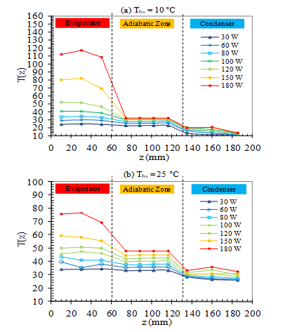
The axial temperature distribution along the heat pipe, for different input powers are illustrated in Figure 8. The heat pipe is horizontally oriented and the heat sink temperature, Ths, is set to 10 °C, 25 °C, 35 °C, and 45 °C, respectively. For a given power, we distinguish three types of the axial wall temperature evolution. Along the zone of evaporation, the wall temperature is the highest and remains nearly constant. From the evaporator to the adiabatic zone, the axial temperature decreases and remains practically constant along the adiabatic zone. From the adiabatic zone to the condenser, the axial temperature also decreases and stabilizes in a constant value along the condensation zone. The temperature gradient along the heat pipe illustrates the ability of the heat pipe to transfer heat in different areas. The axial distribution of the temperature depends on the heat input power and on the heat sink temperature, Ths. Note that for input powers exceeding 100 W, the evaporator temperature is no longer constant. Similarly, there is a very significant increase in the evaporator temperature indicating that the capillary limit is exceeded, and the evaporator starts to dry out. The profile of the evaporator temperature becomes parabolic indicating that the heat transfer is carried out by thermal conduction.
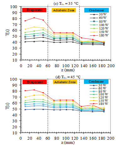
In order to highlight the effectiveness of the heat pipe for this cooling solution, we have carried out experiments on the same cooling system including a cylindrical copper rod instead of a heat pipe. The axial wall temperature distributions along the copper rod are depicted in Figure 9 for a heat sink temperature Ths = 25 °C. As it can be noticed, the evaporator temperatures are higher than those obtained with a heat pipe. Indeed, for a heat input power, Q = 30 W, the evaporator temperature is nearly 150 °C which is obtained for the copper rod-based cooling system; against nearly 34 °C which is obtained with the heat pipe-based cooling system.
Figure 8. Axial wall temperature variations for different heat sink temperatures: (a) 10 °C, (b) 25 °C, (c) 35 °C, (d) 45 °C
The variations of the evaporator, adiabatic and condenser temperatures are depicted in Figure 10. It is observed that evaporator temperature increases sharply for heat input powers higher than 100 W and 120 W when operating at heat sink temperatures equal to 10 °C and 25 °C, respectively (Figure 10a). This indicates that dry-out occurs at the evaporator section. For heat sink temperatures equal to 35 °C and 45 °C, the evaporator temperature increases monotonously without a sharp increase. The adiabatic and condenser temperatures increase monotonously with both the heat input power and the heat sink temperature. It can be noticed that the condenser temperature is higher than the heat sink temperature because of the thermal resistance between the condenser wall and the cooling water.
Figure 9. Axial wall temperature variations for a copper rod-based cooling system (Ths = 25 °C)
Figure 10. Variations of the (a) evaporator, (b) adiabatic, and (c) condenser temperatures as a function of the heat input power for different heat sink temperatures
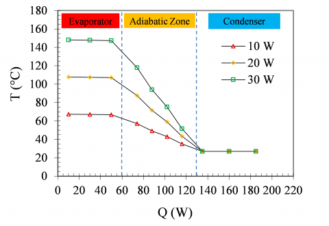
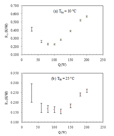
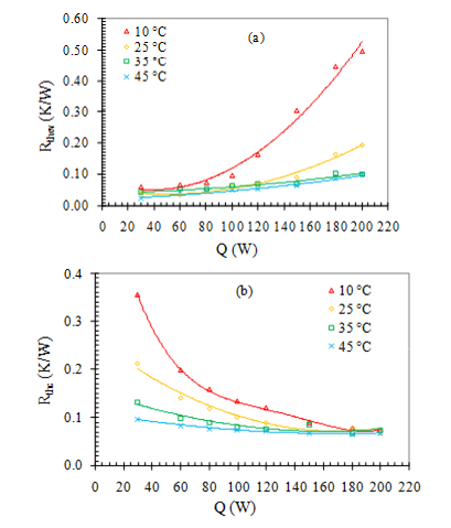
The variations of the overall thermal resistance of the heat pipe with the heat input power for different heat sink temperatures are plotted in Figure 11. For a given heat sink temperature, the heat pipe thermal resistance decreases rapidly to a minimum value as the heat input power increases. This minimum value corresponds to the capillary limit. It corresponds to the maximum heat input power that the heat pipe can transport before dry-out in the evaporator starts. The capillary limit depends on the heat sink temperature. Indeed, for Ths = 10 °C, the maximum heat flux rate that the heat pipe can transport is approximately 80 W. However, the capillary limit is equal nearly to 100 W, 110 W, and 120 W for Ths = 25 °C, Ths = 35 °C, and Ths = 45 °C, respectively. This shows that the heat transfer is enhanced when the heat sink temperature increases. This is also demonstrated by the decrease of the heat pipe thermal resistance. For heat input powers exceeding the capillary limit, the thermal resistance starts to increase showing heat transfer degradation. This is due mainly to the beginning of the dry-out in the evaporator and flooding in the condenser.
Figure 11. Overall thermal resistance variations vs. heat input, for different heat sink temperatures: (a) 10 °C, (b) 25 °C, (c) 35 °C, and (d) 45 °C
Figure 12 illustrates the variations of the evaporator and condenser thermal resistances as a function of the heat input power, for different heat sink temperatures. They are calculated by Eqns. (2) and (3). For a given heat sink temperature, the evaporator thermal resistance increases with the heat input (Figure 12a). The degradation of the evaporation process is caused by the fact that the evaporator becomes starved of liquid since the capillary pumping pressure becomes insufficient to overcome the liquid and vapor pressure losses when the heat input increases. For given heat input, the evaporator thermal resistance decreases as the heat sink temperature increases. This is because augmenting the heat sink temperature causes an increase of the saturation temperature and pressure. Hence, the evaporation process is enhanced. The condenser thermal resistance decreases with the heat input power (Figure 12b). Indeed, increasing the heat input power causes an augmentation of the liquid mass flow rate along the condenser, and the condensation process is enhanced. These results clearly indicate that the heat pipe is correctly filled, and the flooding zone can be considered as negligible. For a given heat input power, the condenser thermal resistance decreases when the heat sink temperature increases. Hence, the condensation process is enhanced.
Figure 12. Variations of the evaporator and condenser thermal resistances as a function of the heat input power, for different heat sink temperatures: (a) evaporator thermal resistance, (b) condenser thermal resistance
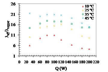
In order to highlight the effectiveness of the heat pipe heat transfer capacity, we have proceeded in calculating the ratio of its effective thermal conductivity by that of a copper rod (l = 380 W/m.K). Figure 13 shows the variations of this ratio as a function of the heat input power for different heat sink temperatures. The curves present maxima corresponding to the capillary limit. Maximum effective thermal conductivity up to 21 times that of the copper are obtained for a heat sink temperature equal to 45 °C. For a heat sink temperature equal to 10 °C, the effective thermal conductivities are lower than those obtained for Ths = 45 °C, and the maximum effective thermal conductivity is nearly 11 times that of the copper.
Figure 13. Variations of the ratio of the heat pipe effective thermal conductivity to that of a copper rod as a function of the heat input power for different heat sink temperatures
In order to quantify the heat transfer mechanisms in the evaporator and condenser zones, we have processed the experimental data in dimensionless numbers in order to obtain heat transfer laws. The dimensionless analysis is carried out based on Vaschy-Buckingham theorem (or p theorem) [15]. The heat transfer coefficients in the evaporator and condenser zones are calculated according to Eqs(4) and (5). The following dimensionless numbers are evidenced from the p analysis:
(i) the Reynolds number which is defined by
$\operatorname{Re}\text{ }=\text{ }\frac{\text{Q}}{{{\mu }_{l}}\text{ }\pi \text{ }{{\text{D}}_{\text{o}}}\text{ }\Delta {{\text{h}}_{\text{v}}}}$ (18)
ml is the liquid dynamic viscosity, and Dhv is the latent heat of vaporization. Do is the heat pipe outer diameter, and Q is the heat flux rate.
(ii) thePrandtl number
$\Pr \text{ }=\text{ }\frac{{{\mu }_{\text{l }}}{{c}_{pl}}}{{{\lambda }_{\text{l}}}}$ (19)
cpl is the liquid specific heat, and ll is the liquid thermal conductivity.
(iii) the Nusselt number
$N{{u}_{{}}}\text{ }=\text{ }\frac{{{\text{h}}_{\text{ }}}L}{{{\lambda }_{l}}}\text{ }$ (20)
h is the heat transfer coefficient for evaporation or condensation, and L is a reference length which is expressed as
For evaporation
${{L}_{(ev)}}\text{ }=\text{ }\sqrt{\frac{\sigma }{\left( {{\rho }_{l}}-\text{ }{{\rho }_{v}} \right)\text{g}}}$ (21)
For condensation
${{L}_{(c)}}\text{ }=\text{ }{{\left( \frac{\nu _{l}^{2}}{\text{g}} \right)}^{{1}/{3}\;}}$ (22)
s is the liquid surface tension. rl and rv are the liquid and vapor densities, respectively. nl is the kinematic viscosity, and g is the gravity acceleration.
(iv) the modified Jackob number
$Ja*\text{ }=\text{ }\frac{{{\rho }_{\text{l}}}}{{{\rho }_{\text{v}}}}\text{ }\frac{{{\text{c}}_{\text{pl}}}\text{ }{{\text{T}}_{\text{sat}}}}{\Delta {{\text{h}}_{\text{v}}}}$ (23)
Tsat is the saturation temperature.
(v) the Kutateladze number
${{\text{K}}_{\text{p}}}\text{ }=\text{ }\frac{{{\text{P}}_{\text{sat}}}\text{ }{{\text{L}}_{\text{(ev)}}}}{\sigma }$ (24)
Hence, the heat transfer coefficients can be calculated by the following correlation
$Nu\text{ }=\text{ A R}{{\text{e}}^{{{\text{m}}_{\text{1}}}}}\text{ P}{{\text{r}}^{{{\text{m}}_{\text{2}}}}}\text{ Ja}{{\text{*}}^{{{\text{m}}_{\text{3}}}}}\text{K}_{\text{p}}^{{{\text{m}}_{\text{4}}}}$ (25)
A, m1, m2, and m3 are constants, which are determined from the experimental results. For the evaporation heat transfer, the dimensionless numbers are determined by calculating the liquid physical properties at the saturation temperature and the vapor physical properties at the film temperature (Tf = (Tsat+ Tw)/2). For the condensation heat transfer, the liquid and vapor physical properties are determined by considering the film and saturation temperatures, respectively.
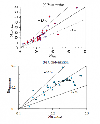
The constants of Eq. (25) are determined by a linear regression analysis, for the evaporation and the condensation phenomena. The experimental results are well correlated when considering A = 339.3, m1 = -0.978, m2 = -0.968, m3 = 0.205, and m4 = 1.586, for the evaporation phenomenon, and A = 10.1, m1 = 0.384, m2 = - 1.738, m3 = - 1.099, and m4 = 0, for the condensation phenomenon. The variations of the calculated Nusselt number as a function of the Nusselt number obtained experimentally are depicted in Figure 14. As it can be seen, the experimental Nusselt number for the heat transfer by evaporation and condensation are well correlated by Eq. (25). The deviations from the experimental results are± 35% and ± 30 % for the evaporation and condensation heat transfer, respectively. The validity of Eq. (25) is insured for the dimensionless numbers ranging in the intervals listed in Table 6.
Table 6. Range of the dimensionless numbers in Eq. (25)
|
Evaporation |
Condensation |
|
1 ≤ Re ≤ 16 |
0.24≤ Re ≤ 3.6 |
|
2.7 ≤Pr≤ 6.6 |
2.9 ≤Pr≤ 7.5 |
|
1 ≤Kp≤ 16 |
1.4 ≤Kp≤ 7.5 |
|
127 ≤Ja* ≤ 11,628 |
|
Figure 14. Variations of the Nusselt number obtained from the experimental results and that calculated by Eq. (25): (a) case of the evaporation, and (b) case of the condensation
5.1 Modeling of the capillary limit
The proper operation of the heat pipe is insured when the capillary pumping, DPc, is capable to overcome the pressure losses in the liquid and vapor phases, DPl and DPv, as well as the hydrostatic pressure, DPg, according to
$\Delta {{P}_{c}}\ge \text{ }\Delta {{{P}}_{{l}}}+\Delta {{P}_{v}}+\Delta {{P}_{g}}$ (26)
The driving capillary pressure can be expressed by
$\Delta {{P}_{c}}{ = 2 }\sigma \text{ cos}\left( \theta \right)\text{ }\left( \frac{1}{{{\text{r}}_{\text{ce}}}}-\frac{1}{{{r}_{cc}}} \right)\text{ }$ (27)
s is the surface tension and q is the contact angle. rce and rcc are the minimum and the maximum capillary radii in the evaporator and condenser sections, respectively. They are given by the following expressions
${{r}_{ce}}=\frac{{{D}_{g}}}{1+\sin \left( \beta +\theta \right)}$ (28)
${{r}_{cc}}=\frac{{{D}_{g}}\tan \left( \beta \right)+0.5\text{ }{{W}_{gb}}}{\cos \left( \beta +\theta \right)}$ (29)
The pressure losses in the liquid and vapor phases are written as [16]
$\Delta {{P}_{v}}\text{ = }{{\text{F}}_{_{\text{v}}}}{{\text{L}}_{\text{eff}}}\text{ Q }$ (30)
$\Delta {{P}_{l}}\text{ = }{{\text{F}}_{_{\text{l}}}}{{\text{L}}_{\text{eff}}}\text{ Q }$ (31)
Leff is the effective length which is equal to La + 0.5 (Le + Lc) where Le, La, and Lc are the lengths of the evaporation, adiabatic and condensation zones, respectively. Fv and Fl are the friction coefficients in the vapor and liquid phases, and Q is the heat input power.
The axial and radial hydrostatic pressures are expressed as follows [16]
$\Delta {{P}_{g,axial}}\text{ = }{{\rho }_{\text{l}}}\text{ g }{{\text{L}}_{\text{t}}}\text{ sin }\left( \psi \right)$ (32)
$\Delta {{P}_{g,radial}}\text{ = }{{\rho }_{\text{l}}}\text{ g }{{\text{D}}_{\text{v}}}\text{ cos }\left( \psi \right)$ (33)
y is the tilt angle with the respect to the horizontal, and Dv is the vapor diameter (Dv = Do – 2 Dg).
Hence, referring to Eq(26), the capillary limit can be expressed as
${{Q}_{\max }}\text{ }=\text{ }\frac{\left( \Delta {{\text{P}}_{\text{c}}}-\Delta {{P}_{g,radial}}\text{ }\pm \Delta {{P}_{g,axial}} \right)}{\left( {{\text{F}}_{\text{l}}}+{{F}_{v}} \right)\text{ }{{\text{L}}_{\text{eff}}}}$ (34)
The sign (+) in the numerator of Eq. (34) corresponds to the thermosyphon position for which the condenser is above the evaporator, and the sign (-) corresponds to the anti-gravity position for which the evaporator is elevated above the condenser.
The vapor friction coefficient, Fv is expressed as [16]
${{F}_{v}}\text{ = }\frac{{{\mu }_{\text{v}}}}{{{K}_{v}}\text{ }{{{{\bar{A}}}}_{\text{v}}}\text{ }{{\rho }_{\text{v}}}\text{ }\Delta {{\text{h}}_{\text{v}}}\text{ }}\text{ }$ (35)
${{{\bar{A}}}_{\text{v}}}$is the mean vapor cross-section, and Kv is the permeability for the vapor flow [16]
${{K}_{v}}\text{ }=\text{ }\frac{\text{D}_{\text{hv}}^{\text{2}}\text{ }}{\text{2 }{{\text{P}}_{\text{ov}}}}$with ${{D}_{\text{hv}}}\text{ }=\text{ }\frac{\text{4 }{{{{\bar{A}}}}_{\text{v}}}\text{ }}{{{\text{p}}_{\text{v}}}}$ (36)
Dhv is the hydraulic diameter of the vapor phase, and Pov is the Poiseuille number which is equal to 16 since the vapor flow is assumed to be circular. pv is the perimeter wetted by the vapor phase.
The liquid friction coefficient, Fl, is given by [16]
${{F}_{l}}\text{ = }\frac{{{\mu }_{\text{l}}}}{{{K}_{g}}\text{ }{{{{\bar{A}}}}_{\text{l}}}\text{ }{{\rho }_{\text{l}}}\text{ }\Delta {{\text{h}}_{\text{v}}}\text{ }}\text{ }$ (37)
Ng is the number of grooves. ${{{\bar{A}}}_{\text{l}}}$is the mean liquid cross-section, and Kg is the groove permeability which is given by the following relation [16]
${{K}_{g}}\text{ }=\text{ }\frac{\text{D}_{\text{hl}}^{\text{2}}\text{ }{{\phi }_{\text{g}}}}{\text{2 }{{\text{P}}_{\text{ol}}}}$with${{D}_{\text{hl}}}\text{ }=\text{ }\frac{\text{4 }{{{{\bar{A}}}}_{\text{l}}}\text{ }}{{{\text{p}}_{\text{l}}}}$ (38)
Dhl is the hydraulic diameter of the liquid phase, and pl is the perimeter wetted by the liquid. φg is the groove porosity which is given by
${{\phi }_{g\text{ }=\text{ }}}\frac{0.5\text{ }{{\text{W}}_{\text{gb}}}\text{ }+\text{ }{{{\text{D}}_{\text{g}}}}/{\tan \left( {\pi }/{2-\beta }\; \right)}\;}{{{W}_{gt}}}$ (39)
The Poiseuille number for the liquid flow, Pol, is calculated as follows [17]
if${{{\text{A}}_{\text{s}}}={{\text{D}}_{\text{g}}}}/{{{W}_{gb}}}\;\text{ }\langle \text{ 1}\text{.5}$
$ P{{o}_{\text{l}}}=\text{ }{{\text{y}}_{\text{o}}}\text{ }+\text{ a }\times \text{ exp}\left( \text{- b }\times \text{ }{{A}_{\text{s}}} \right)\text{ }+\text{ c }\times \text{ }{{A}_{\text{s}}} $
$\left\{\begin{array}{l}{y_{o}=6.391 \theta^{0.121}} \\ {a=137-5.008 \theta+0.07312 \theta^{2}-0.0003808 \theta^{3}} \\ {b=4.901+0.01448 \theta} \\ {c=-0.8141+0.141 \theta-2.762^{-36^{2}}-1.758^{-56^{3}}}\end{array}\right.$ (40)
if${{{\text{A}}_{\text{s}}}={{\text{D}}_{\text{g}}}}/{{{W}_{gb}}}\;\text{ }\rangle \text{ 1}\text{.5}$
$ P{{o}_{l}}\text{ }=\text{ a }\times \text{ exp}\left( \text{-0}\text{.5 }\times \text{ }{{\left( \text{log}\left( {{{A}_{s}}}/{{{\text{x}}_{\text{o}}}}\; \right)/b \right)}^{2}} \right) $
$\left\{\begin{array}{l}{a=11.23 \theta^{0.09313}} \\ {b=2.406 \theta^{0.01303}} \\ {x_{o}=19.29 \theta^{-0.3836}}\end{array}\right.$ (41)
The cross-sectional areas of the liquid and the vapor phases depend on the curvature radius of the meniscus. In Eqns. (35)-(38), the mean values of Al and Av are considered. These values are determined by integrating the local cross-sectional areas along the FMHP, assuming a linear variation of the curvature radius between the value taken in the evaporator section (rce) and that taken in the condenser section (rcc). Hence, ${{ {\bar{A}}}_{\text{l}}}$and ${{ {\bar{A}}}_{\text{v}}}$are expressed as
${{\bar{A}}_{l}}={{a}_{l}}-{{b}_{l}}\text{ }\left( r_{ce}^{2}+{{r}_{ce}}\text{ }{{r}_{cc}}+r_{cc}^{2} \right)$ (42)
${{\bar{A}}_{v}}={{a}_{v}}+{{b}_{v}}\text{ }\left( r_{ce}^{2}+{{r}_{ce}}\text{ }{{r}_{cc}}+r_{cc}^{2} \right)$ (43)
${{a}_{l}}={{N}_{g}}\left( \left( {{W}_{gb}}+{{D}_{g}}\text{ tan}\left( \beta \right) \right)\text{ }{{D}_{g}} \right)$ (44)
${{b}_{l}}={{b}_{v}}={{N}_{g}}\frac{\left( \varphi -\cos \left( \varphi \right)\sin \left( \varphi \right) \right)}{3}$ (45)
${{a}_{v}}=\frac{\pi \text{ }D_{v}^{2}}{4}$ (46)
$\varphi \text{ }=\text{ }\frac{\pi }{\text{2}}-\left( \beta +\theta \right)$ (47)
The perimeters pv and pl are expressed by
${{p}_{l}}={{N}_{g}}\left( \frac{2\text{ }{{\text{D}}_{\text{g}}}}{\text{cos}\left( \beta \right)}+{{W}_{gb}} \right)$ (48)
${{p}_{v}}=\pi \text{ }{{D}_{v}}$ (49)
5.2 Modeling of the heat transfer
The heat exchanges in a heat pipe are of various natures and they can be represented by the thermal resistance network shown in Figure 15. We can distinguish the thermal resistances, R1 and R7, due to the radial conduction through the evaporator and the condenser walls, the thermal resistance, R8, due to the axial conduction along the heat pipe wall, the thermal resistances, R2 and R6, due to the evaporation and condensation, the thermal resistances R3 and R5 due to the heat exchanges by phase change at the liquid-vapor interfaces, and the thermal resistance R4 due to the exchanges by convection between the vapor and the heat pipe wall.
Figure 15. Thermal resistance network representing the heat exchanges in the heat pipe
By supposing that the thermal resistance, R8, due to the axial conduction along the heat pipe is high, the heat pipe overall thermal resistance, Rtht can be expressed by
${{R}_{tht}}\text{ }=\text{ }\sum\limits_{\text{i}=\text{1}}^{\text{7}}{{{\text{R}}_{\text{i}}}}$ (50)
The thermal resistances R3 and R5 are expressed by [16]
$R_{3}^{{}}=R_{5}^{{}}=\frac{{{T}_{sat}}\sqrt{2\pi \text{ }r\text{ }{{T}_{sat}}}}{{{\rho }_{l}}\text{ }\Delta h_{v}^{2}}\frac{(2-{{a}_{c}})}{{{a}_{c}}}$ (51)
ac is the accommodation coefficient and r is the gas constant.
The thermal resistance R4 is given by [16]
${{R}_{4}}\text{ }=\text{ }\frac{{{\text{T}}_{\text{sat}}}\text{ }\Delta {{\text{P}}_{\text{v}}}}{{{\rho }_{\text{v}}}\text{ }\Delta {{h}_{v}}\text{ Q}}$ (52)
The wall thermal resistances, R1,7, are given by
${{R}_{1,7}}\text{ }=\text{ }\frac{\text{1}}{\text{2 }\pi \text{ }\lambda {{\text{ }}_{\text{w }}}\ell }\text{ ln}\left( \frac{{{\text{D}}_{\text{o}}}}{{{\text{D}}_{\text{i}}}} \right)$ (53)
Do et Di are the outer and inner diameters, respectively. lw is the wall thermal conductivity. R1and R7 are calculated by taking $\ell \text{ }=\text{ }{{\text{L}}_{\text{e}}}$ and $\ell \text{ }=\text{ }{{\text{L}}_{\text{c}}}$, respectively.
R2 and R6 are calculated according to
${{R}_{2}}\text{ }=\text{ }\frac{\text{1}}{{{\text{h}}_{\text{ev}}}\text{ }{{\text{A}}_{\text{ev}}}}$ (54)
${{R}_{6}}\text{ }=\text{ }\frac{\text{1}}{{{\text{h}}_{\text{c}}}\text{ }{{\text{A}}_{\text{c}}}}$ (55)
hev and hc are the heat transfer coefficient of evaporation and condensation, respectively. They are determined from Eq. (25). Aev and Ac are the evaporator and condensation heat transfer areas, respectively.
5.3 Calculation procedure
The calculation procedure is as follows:
${{T}_{satcalculated}}=\text{ }{{\text{T}}_{\text{wc}}}+\left( {{R}_{5}}+{{R}_{6}}+{{R}_{7}} \right)\text{ }{{\text{Q}}_{\text{max}}}$ (56)
${{T}_{ev}}=\text{ }{{\text{T}}_{\text{sat}}}+\left( {{R}_{1}}+{{R}_{2}}+{{R}_{3}} \right)\text{ }{{\text{Q}}_{\text{max}}}$ (57)
5.4 Comparison between the model results and the experimental data
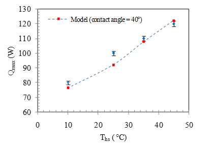
The variations of the capillary limit, Qmax, obtained experimentally and that obtained theoretically from the model are depicted in Figure 16. The capillary limit increases with the heat sink temperature. This is mainly due to the decrease of the liquid pressure drop with the temperature (the vapor pressure drop is very negligible compared to the liquid one). The relative discrepancy between the experimental data and the calculated ones ranges between -1.7 % and +7.9 % indicating a very good agreement if we take into consideration the uncertainty on the experimental results. Note that this agreement depends on the value of the contact angle that is considered in the model. The value of the contact angle, which gives the best agreement, is 40 °.
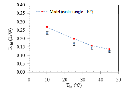
The variations of the overall heat pipe thermal resistance, Rtht, corresponding to the capillary limit, Qmax, are plotted in Figure 17. A good agreement is obtained between the experimental results and those determined from the model. Hence, the relative discrepancy between the experimental results and those issued from the model ranges between -1.7 % and + 7.9 %.
Figure 16. Variations of Qmax as a function of Ths
The variations of the evaporator wall temperature, Twev, are depicted in Figure 18. Twev increases with Ths and a good agreement is obtained between the experimental results and those calculated from the model. The relative discrepancy ranges between +4.4 % and 9.5 % indicating that the model overestimates slightly the experimental results.
Figure 17. Variations of Rtht as a function of Ths
Figure 18. Variations of Twev as a function of Ths
In this study, a copper-water cylindrical heat pipe was manufactured and tested in order to determine its thermal performance for different heat sink temperatures and the heat input powers. For a given heat sink temperature, it is demonstrated that the evaporation process is altered when the heat input power increases. However, the condensation process is enhanced when the heat input power increases. Furthermore, both the evaporation and condensation processes are enhanced when the heat sink temperature increases whatever the heat input power. Heat transfer laws are proposed based on a dimensionless analysis of the evaporation and condensation phenomena. A model is developed in order to determine the capillary limit as well the heat transfer within the heat pipe. The model can predict the experimental results within -1.7 % and +7.9 % when estimating the capillary limit and underestimates the heat pipe overall thermal resistance within -17.8 % and -9.7 % and overestimates the evaporator temperature within 4.4 % and 9.5 %.
|
a |
parameter defined in Eqns. (40) and (41) |
|
A |
constant in Eq. (25) |
|
ac |
accommodation coefficient |
|
Ac |
inner area of the condenser section, m² |
|
Aev |
inner area of the evaporator section, m² |
|
As |
aspect ratio |
|
al |
parameter defined by Eq. (44) |
|
av |
Parameter defined by Eq. (46) |
|
${{{\bar{A}}}_{{v}}}$ |
mean vapor cross-section, m² |
|
${{{\bar{A}}}_{{l}}}$ |
mean liquid cross-section, m² |
|
b |
parameter defined by Eqns. (40) and (41) |
|
B |
bias limit contribution |
|
bl |
parameter defined by Eq. (45) |
|
bv |
parameter defined by Eq. (45) |
|
c |
parameter defined by Eqns. (40) and (41) |
|
cp |
specific heat, J. kg-1. K-1 |
|
Do |
outer diameter, m |
|
Dg |
groove depth, m |
|
DHL |
hydraulic diameter of the liquid phase, m |
|
Dhv |
hydraulic diameter of the vapor phase, m |
|
Dv |
vapor diameter, m |
|
F |
friction factor, Pa/W.m |
|
g |
gravitational acceleration, m/s² |
|
hc |
heat transfer coefficient of condensation, W/m².K |
|
hev |
heat transfer coefficient of evaporation, W/m².K |
|
Ja* |
modified Jackob number |
|
K |
permeability, m2 |
|
Kp |
Kutateladze number |
|
L |
reference length, m |
|
Lc |
condenser length, m |
|
Le |
evaporator length, m |
|
Leff |
effective length, m |
|
Lt |
overall length of the heat pipe, m |
|
m1, m2, m3, m4 |
constants in Eq. (25) |
|
Ng |
number of grooves |
|
Nu |
Nusselt number |
|
p |
perimeter, m |
|
P |
precision limit contribution |
|
Po |
Poiseuille number |
|
Psat |
saturation temperature, Pa |
|
Q |
heat input power, W |
|
qc |
heat flux at the condenser section, W/m² |
|
qev |
heat flux at the evaporator section, W/m² |
|
r |
gaz constant, J/kg.K |
|
R1 |
thermal resistance due to thermal conduction through the evaporator wall, K/W |
|
R2 |
thermal resistance due to evaporation, K/W |
|
R3 |
liquid-vapor interfacial thermal resistance, K/W |
|
R4 |
thermal resistance due to the exchanges between the vapor and the heat pipe wall, K/W |
|
R5 |
liquid-vapor interfacial thermal resistance, K/W |
|
R6 |
thermal resistance due to condensation, K/W |
|
R7 |
thermal resistance due to thermal conduction through the condensation wall, K/W |
|
R8 |
thermal resistance due thermal conduction along the heat pipe, K/W |
|
rc |
capillary radius, m |
|
Re |
Reynolds number |
|
Rth |
heat pipe overall thermal resistance, K/W |
|
Rtha |
thermal resistance of the adiabatic zone, K/W |
|
Rthc |
condenser thermal resistance, K/W |
|
Rthcond |
thermal resistance of condensation, K/W |
|
Rthev |
evaporator thermal resistance, K/W |
|
Rthevap |
thermal resistance of evaporation, K/W |
|
Rthwallc |
thermal resistance of the condenser wall, K/W |
|
Rthwallev |
thermal resistance of the evaporator wall, K/W |
|
Sg |
groove spacing, m |
|
${{{\bar{T}}}_{{ad}}}$ |
average temperature of the adiabatic zone, °C |
|
${{{\bar{T}}}_{{c}}}$ |
average temperature of the condenser, °C |
|
${{{\bar{T}}}_{{ev}}}$ |
average temperature of the evaporator, °C |
|
Tf |
film temperature, °C |
|
Ths |
heat sink temperature, °C |
|
Tw |
wall temperature, °C |
|
Tsat |
saturation temperature, °C |
|
tw |
wall thickness, m |
|
Wgb |
width at the base of the groove, m |
|
Wgt |
width at the top of the groove, m |
|
xo |
constant defined by Eqns. (40) and (41) |
|
Greek symbols |
|
|
a |
angle defined in Figure 2, ° |
|
b |
angle defined in Figure 2, ° |
|
$\Delta {{{h}}_{{v}}}$ |
latent heat of vaporization, J/kg |
|
$\Delta {{{P}}_{{c}}}$ |
capillary pressure, Pa |
|
$\Delta {{{P}}_{{g}}}$ |
hydrostatic pressure, Pa |
|
$\Delta {{{P}}_{{l}}}$ |
liquid pressure loss, Pa |
|
$\Delta {{{P}}_{{v}}}$ |
vapor pressure loss, Pa |
|
$\Delta {{{\bar{T}}}_{{c}}}$ |
average temperature difference between the condenser and the adiabatic sections, K |
|
$\Delta {{{\bar{T}}}_{{ev}}}$ |
average temperature difference between the evaporator and adiabatic sections, K |
|
$\Delta {{{\bar{T}}}_{{hp}}}$ |
average temperature difference between the evaporator and condenser sections, K |
|
|
angle defined in Figure 3, ° |
|
θ |
contact angle, ° |
|
λ |
thermal conductivity, W/m.K |
|
µ |
dynamic viscosity, kg. m-1.s-1 |
|
ν |
kinematic viscosity, m/s² |
|
ρ |
density, kg/m3 |
|
σ |
surface tension, N/m |
|
φ |
porosity |
|
Subscripts |
|
|
ad |
adiabatic |
|
c |
condenser, condensation |
|
cond |
condensation |
|
e |
evaporator |
|
ev |
evaporator, evaporation |
|
evap |
evaporation |
|
g |
groove, hydrostatic |
|
gb |
groove bottom |
|
gt |
groove top |
|
hp |
heat pipe |
|
hs |
heat sink |
|
i |
inner |
|
l |
liquid |
|
max |
maximum |
|
o |
outer |
|
sat |
saturation |
|
t |
overall |
|
v |
vapor |
|
w |
wall |
[1] Tathgir RG, Singh G. (1983). Experimental study of a grooved heat pipe at moderate temperature range. Journal of Institution of Engineers (India): Mechanical Engineering division 64(3): 116-119.
[2] Schlitt R. (1995). Performance characteristics of recently developed high-performance heat pipes. Heat Transfer Engineering 16(1): 44-52. https://doi.org/10.1080/01457639508939844
[3] Lataoui Z, Romestant C, Bertin Y, Jemni A, Petit D. (2008). Experimental investigation on the thermal behavior and performance of an axially grooved heat pipe. International Journal of Heat and Technology 26(2): 155-162.
[4] Zhang C, Shi M, Wu J. (2008). Flow and heat transfer characteristics of heat with axial “Ω” shaped grooves. Journal of Chemical Industry and Engineering (China) 59(3): 544-550.
[5] Zhu WF, Chen YP, Zhang CB, Shi M. (2009). Flowing and heat transfer characteristics of heat pipe with axially shallow-tailed microgrooves. Journal of Astronautics 30(6): 2380-2386.
[6] Yao F, Chen YP, Zhang CB, Shi MH. (2011). Startup characteristics of heat pipe with axially “Ω” shaped grooves. Journal of Engineering Thermophysics 32(12): 2117-2119.
[7] Yang KM, Wang NH, Jiang CH, Cheng L. (2012). An investigation of the thermal performance of a novel axial grooved heat pipe. Advanced Materials Research 580: 223-226. https://doi.org/10.4028/www.scientific.net/amr.580.223
[8] Yang KM, Wang NH, Jiang CH, Cheng L. (2012). Study on heat transfer characteristics of heat pipe with axial “Ω” shaped microgrooves. Advances Materials Research 580: 297-300. https://doi.org/10.4028/www.scientific.net/amr.580.297
[9] Bertoldo Junior J, Vlassov VV, Genaro G, Tuden Viera Gedes U. (2015). Dynamic test method to determine the capillary limit of axially grooved heat pipes. Experimental Thermal Sciences 60: 290-298. https://doi.org/10.1016/j.expthermflusci.2014.10.002
[10] Driss A, Maalej S, Zaghdoudi MC. (2016). Experimentation and modeling of the steady-state and transient thermal performances of a helicoidally grooved cylindrical heat pipe. Microelectronics Reliability 62: 102-112. https://doi.org/10.1016/j.microrel.2016.03.022
[11] Yang K, Mao Y, Cong Z, Zhang X. (2017). Experimental research of novel aluminum-ammonia heat pipes. Procedia Engineering 205: 3923-3930. https://doi.org/10.1016/j.proeng.2017.10.032
[12] Pis’mennyi EN, Khayrnasov SM, Rassamakin BM. (2018). Heat transfer in the evaporation zone of aluminum grooved heat pipes. Int. J. Heat and Mass Transfer 127: 80-88. https://doi.org/10.1016/j.ijheatmasstransfer.2018.07.154
[13] Ömür C, Bilge Uygur A, Howz I, GürgüçIsik H, Ayan S, Konar M. (2018). Incorporating of manufacturing constraints into an algorithm for the determination of maximum heat transport capacity of extruded axially grooved heat pipes. International Journal of Thermal Sciences 123: 181-190. https://doi.org/10.1016/j.ijthermalsci.2017.09.016
[14] Kline SJ, McClintock FA. (1953). The description of uncertainties in single sample experiments. Mechanical Engineering, ASME 75: 3-8.
[15] Mansouri J, Maalej S, Sassi MBH, Zaghdoudi MC. (2011). Experimental study on the thermal performance of enhanced flat miniature heat pipes. International Review of Mechanical Engineering 5(1): 196-208.
[16] Faghri A. (1995). Heat pipe science and technology. 1st Edition. Taylor and Francis.
[17] Kim SJ, Seo JK, Do KH. (2003). Analytical and experimental investigation of the operational characteristics and the thermal optimization of a miniature heat pipe with a grooved wick structure. Int. J. Heat and Mass Transfer 46: 2051-2063. https://doi.org/10.1016/S0017-9310(02)00504-5