OPEN ACCESS
Shovel-Dumper system is utilized as a loading and transporting machines for intermediate mechanization in surface mining. For survival in the exceptional competition in the global business environment in recent years, it is basic that the Shovel – Dumper system should be reliable and maintained adequately and effectively. This paper seeks to study the reliability, availability, and preventive maintenance of one shovel and four dumpers in a surface coal mine with failure and repair data by Isograph Reliability Workbench (RWB) in the case of a non-parametric statistical method such as K-S test. The constraints and reasons for machine unavailability are outlined. The reliability and availability of the shovel-dumper system are evaluated and also evaluated the maintenance time interval to improve the 80% of reliability for each system. The reliability, availability and preventive maintenance have been validated with the artificial neural network (ANN). ANN model is then connected to a reliability method, K-S test to predict the failure probability of shovel and dumper.
shovel-dumper system, surface coal mine, reliability, availability, maintainability, K-S test and ANN
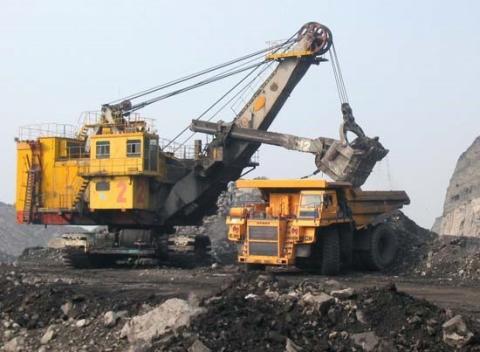
Shovels and dumpers are the major machineries under HEMM mainly used for loading and transportation of excavated ores and minerals in surface coal mines as shown in figure 1. With regular use of shovels and dumpers productivity is increased. But the efficient increase in productivity can be achieved through of effective use of shovels and dumpers [1].
Figure 1. Shovel-Dumper combination
In this article, two methods are used to conduct the reliability, availability and preventive maintenance analysis. They are, i) a basic maintenance technique, ii) a reliability-based technique [1]. First, the basic maintenance technique is used to determine mean time between failure (MTBF) by the use of the failure data and mean time to repair (MTTR) via using repair data of shovel and dumper below case observe. Then, the reliability-based technique is used to shows the reliability improvement in shovel and dumpers by way of the usage of Weibull distribution modelling strategies [2]. As a result of this study, suggestions for the implementation of a preventive maintenance time interval may be suggested and considered by using mines management to improve the reliability of shovels and dumpers in a surface coal mine using Isograph Reliability workbench and validate with ANN tool [3].
The Weibull Module of RWB allows to import historical failure data, fit the data with a relevant distribution and use the resulting fit parameters as failure data in the reliability function. The historical data is stored in a Weibull Set object, which can be allocated to one or more Failure Models. The Shovel-Dumper system in surface mines can fail due to subsytems such as engine, hydropneumatuc suspension system, electrical subsystem and etc. A record has been kept of each failure in the form of a list of times to failure. Now import these times to failure into a Weibull Set and perform a line fit analysis [4].
Begin by opening the file Tutorial.rwb. Select the Weibull module from the Module pull-down menu. The Reliability Workbench window is now set up for the Weibull Module. The left pane will display the Weibull sets available. The top right pane will display the Cumulative Probability plot. This will be blank until the historical failure data is imported. The bottom right pane is a grid control set to display the historical failure data [4].
Select the Add, Weibull Set pull-down menu option or equivalent toolbar button. The Weibull Set Properties dialog will appear. Enter an ID of “S1” and a description ‘failure mode”. Click OK to close the dialog and save changes. The new Weibull Set will now appear beneath the Weibull Sets node in the Tree Control. Similarly for D1, D2, D3 and D4 [4].
Select the Column Matches tab. Left click on TTF in the External Columns column and then left click on TimeValue in the Application Columns column. This creates a link between the column of data on the clipboard and the appropriate column of the project data table. . Now click on the Auto Match button at the bottom of the dialog to match the remaining columns by name. Click Import to populate the S1, D1, D2, D3 and D4 failure data set with the clipboard data. Click OK to close the Import dialog. Do not save an Import/Export template [4].
The data points should now be plotted in the Cumulative Probability plot and the Weibull set items displayed in the grid control. Select the best fit distribution based on from the Distribution selector menu on the toolbar and select the Analysis, Calculate Distribution Parameters Automatically pull-down menu option or equivalent toolbar button. RWB will now perform a line fit analysis of the Weibull data. The results will be displayed in the form of Weibull parameters such as shape parameter, scale parameter and location parameters to the right of the Cumulative Probability plot [4].
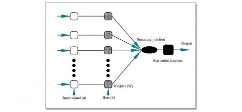
Figure 2. Schematic structure of ANN
Artificial Neural Network (ANN) in MATLAB is a simulation tool, designed to work with comparative functionalities as that of the human brain [3]. It is an intricate handling processing system that can develop outputs based on the nature and kind of inputs fed. An ANN show comprises of three layers: with First as an information layer, last as yield layer and the centre as a shrouded layer. In feed-forward systems demonstrated in figure 2, each result of enter components (ai) and weights (wij) are nourished to adding intersections and is added with bias (bj) of neurons as follows equation (1) [3, 5]:
$X=\left(\sum_{i=1}^{n} w_{i j} a_{i}\right)+b_{j}$ (1)
Then this summation (X) passes throughout transfer function (F) which generates an output using equation (2) [3, 5].
$F(X)=\mathbf{u}_{\mathrm{j}}=\mathrm{F}\left[\sum_{\mathrm{i}=1}^{\mathrm{n}}\left(w_{i j} a_{i}\right)+\mathrm{b}_{\mathrm{j}}\right]$ (2)
In the hidden layer, the most commonly used transfer functions are Tansig and logsig. The nonlinear activation function that is commonly applied is known as a sigmoid function whose yield lies inside the mid of zero and one, and the sigmoid transfer function is written as equation (3) [3, 5].
$F(X)=\frac{1}{1+\mathrm{e}^{-\mathrm{x}}}$ (3)
The obtained values of Isograph Reliability Workbench and the predicated values of the ANN are interpolated using biases and weights of the network in order to minimize the error between them.
The location of the study mine is Open Cast-I (OC-I), The Singareni Collieries Company Limited, Kothagudem area, Telangana. The mine used a number of shovels and dumpers of different makes (Komatsu and BEML) having different capacities. The rated capacities of shovels included 12, 11 & 6.5 cubic meters and that of dumpers included 100 T, 65 T & 35 T. In this article one shovel (S1: Komatsu shovel, capacity: 12 cubic meters) and four dumpers (D1, D2: BEML dumper & D3, D4: Komatsu Dumper, capacity: 100 Tones each) were considered based on the match factor i.e., 1:4. In this case study, the field data namely, failure frequency, MTBF and MTTR of the shovel-dumper system (S1, D1, D2, D3 and D4) were collected for the period of the 1 year as shown in table 1.
Table 1. Collected failure data for a shovel and dumpers
|
Systems |
Failure Frequency |
MTBF in hr |
MTTR in hr |
|
S1 |
181 |
43.71 |
4.69 |
|
D1 |
54 |
117.35 |
39.08 |
|
D2 |
46 |
138.48 |
51.96 |
|
D3 |
88 |
78.42 |
21.13 |
|
D4 |
141 |
54.80 |
7.33 |
Based on the collected failure date of the shovel-dumper system in the surface coal mine, the availability was calculated using following equation (4) [2] and obtained values of availability of a shovel and each dumper has mentioned in table 2. The table 2 says that availability of the S1 and D4 in the surface coal mine is 0.90 & 0.88 respectively because of good maintainability. The availability of S1 and D4 is comparatively better than the other system such as D1, D2 and D3. Due to the more failure frequency of D1, D2 and D3, the availability of these systems are less about 0.75, 0.73 and 0.78 respectively even they have good maintainability [6].
Availability$=\frac{M T B F}{(M T B F+M T T R)}$ (4)
Table 2. Availability of a shovel and each dumper
|
Systems |
Failure Frequency |
MTBF in hr |
MTTR in hr |
Availability |
|
S1 |
181 |
43.71 |
4.69 |
0.90 |
|
D1 |
54 |
117.35 |
39.08 |
0.75 |
|
D2 |
46 |
138.48 |
51.96 |
0.73 |
|
D3 |
88 |
78.42 |
21.13 |
0.79 |
|
D4 |
141 |
54.80 |
7.33 |
0.88 |
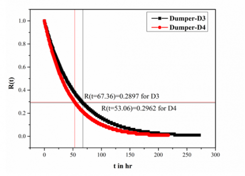
Reliability of a shovel (S1) and each dumper (D1, D2, D3 & D4) were determined for particular MTBF from the corresponding best fit probability distribution function, such as Weibull distribution using equation (5) [1, 6] is tabulated as shown in table 3. The reliability difference between S1, D1, D2, S3, and S4 is increasing and decreasing as the machine time increases. The results are also shown graphically in figure 3 for S1, figure 4 for D1 & D2 and figure 5 for D3 & D4. The figure 3, 4 & 5 clearly says that, if working hours increases, the reliability of the shovel and dumper system in the surface coal mine will decrease gradually.
$R(t)=e^{-\left(\frac{t-\lambda}{\eta}\right)^{\beta}}$ (5)
Table 3. Weibull parameter and reliability function (R(t))
|
S. No |
Systems |
MTBF in hr |
Best Fit distribution |
Parameters |
R (t) |
||
|
h |
b |
g |
|||||
|
1 |
S1 |
43.71 |
Weibull 2P |
29.83 |
0.7139 |
0 |
0.2682 |
|
2 |
D1 |
117.35 |
Weibull 3P |
115.7 |
1.018 |
-3.967 |
0.3731 |
|
3 |
D2 |
138.48 |
Weibull 3P |
83.12 |
0.5357 |
-0.2365 |
0.2850 |
|
4 |
D3 |
78.42 |
Weibull 1P |
54.37 |
1 |
0 |
0.2897 |
|
5 |
D4 |
54.80 |
Weibull 1P |
43.61 |
1 |
0 |
0.2962 |
Figure 4. Reliability estimation of the dumpers (D1 & D2)
The preventive maintenance is required to improve the reliability of any system or machine. Since the reliability of a shovel and each dumper were different so that the preventive maintenance time interval for each subsystem will also be different [7-8]. The maintenance time interval for each subsystem of a shovel and each dumper were determined to achieve 80 % reliability of systems (shovel & dumper combination) in the surface coal mine using equation (5). The time interval for a shovel and every dumper has been calculated from the corresponding reliability functions. The outcomes are tabulated in table 4. It can be without problems interpreted from the outcomes that, to attain 80% of reliability. The preventive maintenance in hours required for S1, D1, D2, D3 & D4 are 23.71, 26.51, 33.15, 78.86 & 63.25 working hours respectively.
Table 4. Reliability-based time intervals for preventive maintenance of a shovel (S1) and dumpers (D1, D2, D3 & D4) in the coal mine
|
Level of reliability (80 %) |
S1 |
D1 |
D2 |
S3 |
S4 |
|
Preventive Maintenance in hrs |
23.71 |
26.51 |
33.15 |
78.8 |
63.25 |
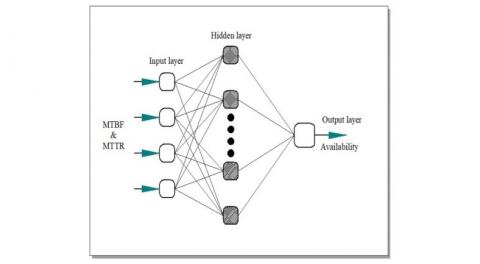
In the present work, availability, reliability and preventive maintenance of one shovel and four dumpers of were taken from the field. The proposed ANN model to predict the availability, reliability and preventive maintenance of a shovel and dumpers in the surface coal mine is shown in figure 6, 7 & 8 respectively. As discussed in section 1, an input layer, two numbers of parameters namely MTBF & MTTR for availability, four number of parameters namely MTBF, shape parameter (b), scale parameter (h) and location parameters (g) for reliability function (R(t)) and four parameters namely R(t), shape parameter (b), scale parameter (h) and location parameters (g) for preventive maintenance for shovel-dumper system has been taken. Similarly, three parameters namely availability, reliability function and preventive maintenance have been taken in the output layer in the ANN model.
Figure 6. ANN model for availability
Figure 7. ANN model for reliability function
Figure 8. ANN model for preventive maintenance
In each model, 5 input and output data collections are taken. In which 3 datasets were utilized for training, 1 dataset for testing and rest one informational index for validation. Feed FB propagation gaining knowledge of algorithm has been related for studying of the current model [5]. Prior to demonstrating the structure of the neural network, the input and output data should be standardized for the precision of the forecast. The following equation (6) has been utilized to standardize information between - 1 and 1[5, 6].
$Y=(High_{Value}-Low_{Value})\frac{Y_i-Y_{Min}}{Y_{Max}-Y_{Min}}+Low_{Value}(6)
In the present investigation, Levenberg - Marquardt back proliferation (LM) learning algorithm was utilized for the training process. The number of neurons in the concealed layer was assessed by trial and error method [5]. Using this technique, 4, 7 and 8 neurons have been selected for availability, reliability function and preventive maintenance respectively with the single hidden layer as shown in figure 6, 7 & 8. LEARNGDM has been chosen, which an adaption is getting to know the function, after the selection of training function. The tansig transfer function selected for the hidden layer and linear function for the output layer.
To minimize the error among the obtained value of Isograph Reliability Workbench and the anticipated predicted values of the ANN model, each neural model trained more than 500 times. This training algorithm adjusts the Wij and bj iteratively. It has been discovered that LM with 4 neurons for availability, 7 neurons for Reliability function and 8 neurons for preventive maintenance is optimize due to minimum error and the maximum value of R2 [5-6, 10]. The execution of various neural models depended on RMSE and R2, which is ascertained by utilizing equation (5) and (6) respectively [9].
$R M S E=\sqrt{\frac{1}{N} \sum_{i=1}^{N}\left(y-y^{\prime}\right)^{2}}$ (7)
$R^{2}=1-\frac{\sum_{i=1}^{N}\left(y-y^{\prime}\right)^{2}}{\sum_{i=1}^{N}\left(y^{\prime}\right)^{2}}$ (8)
6.1 Development and simulation of ANN model for availability
The execution of ANN availability model depended on R2 and RMSE, which is computed by utilizing equation (7) and (8) individually [5]. From Table 5, it has been discovered that estimations of R2 and RMSE are 0.9916 and 0.009623 respectively.
The regression plot of the neural model with LM-4 of training, testing and validation process has appeared in table 5. From table 5, it has been discovered that the estimation of R2 is closer to solidarity i.e., 0.9916, which gives the precision of execution of the model [10].
An examination of the obtained values by Isograph Reliability Workbench with predicated values of ANN model with LM-4 and its errors has appeared in table 8. From table 8, it has been discovered that the maximum error is - 0.00247 at D2 and minimum error is 4.63E-8 at D1 in availability.
Table 5. The training performance of availability for different neurons
|
No. of Neurons |
R2 |
RMSE |
|
2 |
0.9927 |
0.011365 |
|
3 |
0.9951 |
0.009121 |
|
4 |
0.9916 |
0.009623 |
|
5 |
0.9919 |
0.009623 |
|
6 |
0.9949 |
0.098099 |
|
7 |
0.9913 |
0.009724 |
6.2 Development and simulation of ANN model for reliability function
The performance of ANN reliability function model was depended on R2 and RMSE, which is computed by using equations (7) and (8) respectively [5]. From Table 6, it has been discovered that estimations of R2 and RMSE are 0.010272 and 0.9712 respectively.
The regression plot of the neural model with LM-7 of training, testing and validation process has appeared in table 6. From table 6, it has been discovered that the estimation of R2 is closer to solidarity i.e., 0.9712, which gives the exactness of execution of the model [9].
An examination of the obtained values by Isograph Reliability Workbench with predicated values of ANN model with LM-7 and its error has appeared in table 8. From table 8, it has been discovered that the maximum error is 0.026 at D4 and minimum error is 0.00018 at D2 in reliability function.
Table 6. The training performance of the reliability function for different neurons
|
No. of Neurons |
R2 |
RMSE |
|
5 |
0.9932 |
0.01482 |
|
6 |
0.927 |
0.014809 |
|
7 |
0.9712 |
0.010272 |
|
8 |
0.9584 |
0.012378 |
|
9 |
0.9641 |
0.025853 |
|
10 |
0.9574 |
0.014445 |
The performance of ANN preventive maintenance model was depended on R2 and RMSE, which is calculated by using equations (7) and (8) respectively [5]. From Table 7, it has been discovered that estimations of R2 and RMSE are 0.172994 and 0.9507 respectively.
The regression plot of the neural model with LM-8 of training, testing and validation process has appeared in table 6. From table 6, it has been discovered that the estimation of R2 is closer to solidarity i.e., 0.9507, which gives the exactness of execution of the model [9].
A comparison of the obtained values by Isograph Reliability Workbench with predicated values of ANN model with LM-8 and its error has appeared in table 8. From table 8, it has been discovered that the maximum error is - 0.3288 at S1 and minimum error is - 2.53E-6 at D1 in reliability function.
Table 7. The training performance of preventive maintenance for different neurons
|
No. of Neurons |
R2 |
RMSE |
|
5 |
0.9765 |
0.31 |
|
6 |
0.9442 |
0.617189 |
|
7 |
0.9745 |
0.524465 |
|
8 |
0.9507 |
0.172994 |
|
9 |
0.9486 |
0.162331 |
|
S. No |
Systems |
Obtained values by Isograph workbench Reliability |
Predicted Values by ANN |
||||
|
Availability |
Reliability |
Preventive Maintenance |
Availability |
Reliability |
Preventive Maintenance |
||
|
1 |
S1 |
0.8997 |
0.2682 |
23.71 in hr |
0.8997 |
0.2718 |
24.0388 |
|
2 |
D1 |
0.7500 |
0.3731 |
26.51 in hr |
0.7500 |
0.3710 |
26.5100 |
|
3 |
D2 |
0.7325 |
0.2850 |
33.15 in hr |
0.7325 |
0.2832 |
33.3537 |
|
4 |
D3 |
0.7686 |
0.2897 |
78.86 in hr |
0.7686 |
0.2712 |
78.8597 |
|
5 |
D4 |
0.8800 |
0.2962 |
63.25 in hr |
0.8800 |
0.2701 |
63.2500 |
In this paper, availability, reliability and preventive maintenance of one shovel (S1) and four dumpers (D1, D2, D3 & D4) in surface coal were calculated for the period of 1 year. The TBF and TTR data set a shovel and dumpers were found to be Weibull best fit curve using the K-S test. The Weibull distribution provided the best fit in case of all systems i.e., 2 parameter Weibull for S1, 3 Parameter Weibull for D1 & D2, 1Parameter for D3 & D4. The maintenance time interval calculated for 80% of reliability for each system is identified and suggested. And also ANN model has been structured to validating the obtained values with four input parameters MTBF, b, h & g and output parameters availability, reliability function and preventive maintenance. The Levenberg-Marquardt (LM) algorithm with feed-forward backpropagation is used in deriving the optimal present model. The LM learning algorithms with 4 neurons for availability, 7 neurons for reliability function and 8 neurons for preventive maintenance in the hidden layer has been discovered as optimal on the basis of statistical error analysis. The obtained and predicted values of availability, reliability function and preventive maintenance shovel-dumper system in a surface coal mine with the highest R2 value gives satisfactory results.
The authors are grateful to The General Manager (HRD), The Singareni Collieries Company Limited, Kothagudem Collieries for given permission to collect the data and for their kind permission to publish this work. We would also wish to express my gratitude to Dr. Ranjan Kumar, Principal Senior, CIMFR, Dhanbad for giving solution about research work.
TBF Time between failures
TTR Time to repair
MTBF Mean time between failures
RMSE Root mean square error
MLE Maximum likelihood estimation
K-S test Kolmogorov–Smirnov test
FB Propogation Forward back propagation
R(t) Reliability function
Y Obtained values
XA Actual value
XP Predicated value
$\overline{X}$ Average value
Y Obtained value
R2 Coefficient of determinations
bj Bias
Wij Weights
Greek letters
β Shape parameter
η Scale parameter
γ Location parameter
[1] Vayenas N, Wu X. (2009). Maintenance and reliability analysis of a fleet of load-haul-dump vehicles in an underground hard rock mine. Internationa Journal of Mining, Reclamation and Envorornament 23(3): 227-238. https://doi.org/10.1080/17480930902916494
[2] Harish Kumar NS, Choudhary RP, Murthy ChSN. (2018). Failure rate and reliability of the Komatsu hydraulic excavator in surface limestone mine. AIP Conference Proceedings 1-9. https://doi.org/10.1063/1.5029583
[3] Ghritlahre HK, Prasad RK. (2018). Investigation of heat tranfer charectrestics of roughned solar air heater using ANN. International Journal of Heat and Technology 36(1): 102-110. https://doi.org/10.18280/ijht.360114
[4] Anonymous (2013). RWB User Guide, Isograph Reliability Workbench, version13.0, 99-108.
[5] Ghritlahre HK, Prasad RK. (2018). Prediction of exergetic efficiency of arc shaped wire roughened solar air heater using ANN model. International Journal of Heat and Technology 36(3): 1107-1115. https://doi.org/10.18280/ijht.360343
[6] Vagenas N, Runciman N, R.clément S. (1997). A methodology for maintenance analysis of mining equipment. Internationa Journal of Mining, Reclamation and Envorornament 11: 33-40. https://doi.org/10.1080/09208119708944053
[7] Roy SK, Bhattacharyya MM, Naikan VNA. (2001). Maintainability and reliability analysis of a fleet of shovels. Mining Technology 110: 163-171. https://doi.org/10.1179/mnt.2001.110.3.163
[8] Bala RJ, Govinda RM, Murthy ChSN. (2018). Reliability analysis and failure rate evaluation of load haul dump machines using weibull distribution analysis. Mathematical Modelling of Engineering Problems 5(2): 116-122. https://doi.org/10.18280/mmep.050209
[9] Sozen A, Menlik T, Unvar S. (2008). Determination of efficiency of flat-plate solar collectors using neural network approach. Expert Systems with Applications 35(4): 1533-1539. https://doi.org/10.1016/j.eswa.2007.08.080