OPEN ACCESS
This paper reviews the interpretation of phenomena resulting from a thermal effect requires, as a necessary condition, knowledge of the temperature reached. The temperature is added one or more time conditions, whether it is the heating, the temperature stay or the cooling. So can say that the relationship between the heat entering the metal during welding obtain the temperature distribution, the thermal and residual stress. In this work we have measured and calculated the residual stress of the X70 steel welding procedure by the DRX-sinψ2 method before and after relaxation operation on the samples chosen after the estimation of this constraint by the finite element method. Solver, ABAQUS, the result indicates value of residual stress is about 146.67N/mm2 after relaxation and about 96 N/mm2 after relaxation at 0.5h and 50N/mm2 AT 2h.
welding, residual stresses, relaxation, steel X70, Sinψ2 method
The interpretation of phenomena resulting from a thermal effect requires, as a necessary condition, information of the temperature reached. the temperature is added one or more conditions of time, be it heating, temperature stay or cooling. It is necessary to know the thermal welding cycle, that is to say the variation of the temperature T as a function of the time.
In the case of welding of carbon steels, four zones can be distinguished in the joints, according to the maximum temperatures reached:
The melted zone, for which the maximum temperature is greater than or equal to the melting temperature;
The fully austenitic zone, for which the maximum temperature is between the melting temperature TF and the temperature Ac3;
The partially austenitic zone, for which the maximum temperature is between the temperatures Ac3 and Ac1;
The influenced zone, not austenitized, for which the maximum temperature is lower than Ac1.
This phenomena cause elaboration of residual stress. The residual stresses in areas near the weld cause fracture under certain condition. [4]
Many researches to better understand the effect of temperature on welded structure such as, X.K. Zhu, Y.J. Chao [7], Chiaki Shiga and al [8], Mehmet T. Pamuk and al [9], heat treatment influence on welded X70 steel, Kelthoum Digheche et al [10] , BENLAMNOUAR Mohamed Farid, BADJI Riad, HADJI Mohamed [11] as well as the variation and the distribution of the residual stress, Paddea S et al [12] et Wenquan Sun and al [2] constraint evaluation either by DRX as, Z. Boumerzoug and al [13], Dhas & Kumanan [14].
Welding is defined as "a joining process that produces coalescence of materials by heating them to the welding [1].
The heat input to the material being welded. As a result of non-uniform heat distribution and phase transformations occur on the material. These changes generate different residual stress patterns for weld region and also in the heat affected zone (HAZ). [5]
For evaluated the residual stress due to welding we choose the model according to the geometry of the sample studied, and which has undergone various mechanical tests and by numerical approach we will study the thermo mechanical behavior of materials under the effect of welding. The first step is to create a model, the geometry is considered as two thick plates chamfered in opposite V subjected to welding in double pass inner and outer.
The method Sinψ2 to measure the residual stress in crystalline materials has been developed using the value Dq (difference of diffraction in comparison to the theoretical value of the Bragg’s law in crystalline materials)
$\mathrm{n} \lambda=2 \mathrm{d} \sin \theta$ (1)
Where n diffraction order is a whole number, θ is the diffraction angle, d is the interplanar spacing of the family of the diffracted planes and λ is the wavelength.
$\varepsilon=\frac{\Delta \mathrm{d}}{\mathrm{d}}=\cot \theta_{d} \Delta \theta$ (2)
where ε is the deformation rate, θd is the diffraction angle in perfect state (no internal stresses). The applied stress (σ) is then calculated from the following expression:
$\sigma=\frac{\mathrm{E}}{1+v} \frac{\partial(\varepsilon)}{\partial\left(\sin ^{2} \psi\right)}=-\frac{\mathrm{E} \cot \theta_{\mathrm{d}}}{2(1+v)} \frac{\partial(\theta)}{\partial\left(\sin ^{2} \psi\right)}$ (3)
where y is the angle between the normal at the sample surface and that of the diffracting planes. The above equation may be expressed as a product of the constant K (elastic constant for measuring stresses by X-rays) and M is the gradient of the regression line of the data representing the results of the stresses of the different angles y, by using the equation:
$\sigma_{x}=K M$ (4)
With $\mathrm{K}=-\frac{\mathrm{E}}{2(1+v)} \cdot \frac{\pi}{180} \operatorname{ctg} \theta_{0}$ and $M=\frac{\partial\left(2 \theta_{w x}\right)}{\partial\left(\sin ^{2} \psi\right)}$
where θ0 is the diffraction angle when σ is 0, K is a constant of stress measurement, M is a stress measurement factor and σx is stress in x direction [16].
There is a linear relationship between 2θ and Siny2. The slope M can be calculated from three points and more whose coordinates (2θψx, Siny2) based on the determination of these points. The calculation of stresses σx, based on the latter, is exported by measuring the different θψx.
The heat treatment Residual Stresses
In this part, the finite-element method uses the equation of heat conduction. Equation .5 describe the temperature variations in heat treatment processes:
$\frac{\partial}{\partial x}\left(k \frac{\partial T}{\partial x}\right)+\frac{\partial}{\partial y}\left(k \frac{\partial T}{\partial y}\right)+\frac{\partial}{\partial z}\left(k \frac{\partial T}{\partial z}\right)=\rho C \frac{1}{2} \frac{\partial T}{\partial t}$ (5)
where T denotes the temperature, k is the thermal conductivity, C is the specific heat ρ is the density t represent the heat treatment time, z represents the welding direction, x in the transverse direction and y is thickness direction. in addition, convection-conduction boundary conditions
The Heat treatment generates a non-linear thermal gradient and the thermal and mechanical changes arising from the heat source promote thermal stresses and distortions. Therefore, based on the thermal gradients given by Equation (5), The residual stresses based on the deformations caused by the gradients can be determined according to:
σ = δυ λ εkk + 2μ ευ - δυ (3λ+2μ) α T (6)
where λ and μ are the Lame constants, which represent the components of the material deformation due to the temperature and are related to the material elasticity modulus E and Poisson’s ratio υ. The ευ variable is linked to the deformation and displacement according to:
$\varepsilon_{v}=\frac{1}{2}\left(\frac{\partial u_{i}}{\partial x_{j}}+\frac{\partial u_{j}}{\partial x_{i}}\right)$ (7)
The studied material is the steel X70 of the norm API 5L. Its chemical composition is presented in Table 1.
Table 1. Chemical composition of the steel x70 (weight %, max) [6]
|
C |
Si |
Mn |
Ni |
Al |
Cu |
Cr |
Ti |
Nb |
|
0.04 |
0.39 |
1.48 |
0.08 |
0.31 |
0.16 |
0.03 |
0.02 |
0.05 |
Tacked small sample size by the cutting machine (Figure 1), a specimen size 18X10X9 m3 (Figure 2) from 5 API-X70 welded, the surface preparation is very important. for the stress value determined by x-rays may not true stress [15] after chemical etchning by Nital of the weld material has revealed the microsstructures of different zones, i.e, weld seam, heat affected zone (HAZ) and base metal [13]. Heat treatments were applied on welded specimens by isothermal annealing at 550°, 600 and 650 °C during (0.5, 2 and 3 hour).
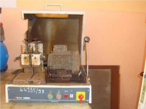
Figure 1. Chainsaw for cutting (struers labotom)
Figure 2. The Photo of Samples cut
Figure 3. Philips X-ray diffractometer photo
You can choose the X-ray diffract (Figure 3) for the residual stress to avoid the influence of the mechanical stress caused by the overflow and using DRX-sinψ2 to estimate the value of the stress before and after the procedure of the relaxation to according the results, residual stress is achieved. Calculated by FEM and measured by X-ray diffract [2].
The angle of orientation of the sample and the normal to the surface of sample was changed between 0°, 45° and 90°, in the experiments. Diffraction peak (211) for X70 steel, for Cu Kα, is located at 2θ = 156° [3].
The effect of repeated thermal cycles, such as the zones whose temperature exceeds the Ac3 undergo a structural regeneration phenomenon, by the transition to the austenitic state on heating, followed by a new transformation on cooling, which erases and replaces the previous structure. The same phenomenon occurred in the ZAT, for estimate the value of residual stress we need based on the components the material parameters and be considered in different temperature by interpolation calculation in ABAQUS [2].
In this model numerical domain is meshed, using tetrahedral with function interpolation quadratic as shown in Figure 4. the gradiant of volume elements used 1×1×1mm and 0.1×0.1×0.1mm.
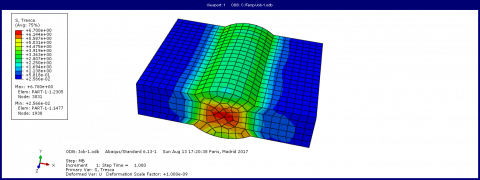
Figure.5-6. present Distribution of stress fields in the specimen under loadings applied according to S.MISES/ S.TRESCA criteria after HT.
Figure 4. Mish grid presentation in the specimen
Figure 5. Distribution of stress fields in the specimen under loadings applied according to S.MISES criteria
Figure 6. Distribution of stress fields in the specimen under loads applied according to S.TRESCA criteria
The treatment was carried out in an electric heating oven with a programming system of temperature cycle. The temperature control is done by electrical regulation. Specimens comprising the base metal and the welded joint were treated at three temperatures, namely 550°, 600° and 650 ° with a hold of (0.5,2 and 3 hour) at this temperature. A heating rate of 185-200C °/h has been applied, as well as the same cooling rate up to 300°, then in the open air of 300 ° to the ambient temperature. The relaxation of the stresses is obtained by the creep of the material, a duration sufficient treatment is required to homogenize the temperature of the welded joint and this, to avoid the creation of new CR at cooling, keeping the temperature of treatment is also essential to ensure the creep relaxation of regions where stress peaks.
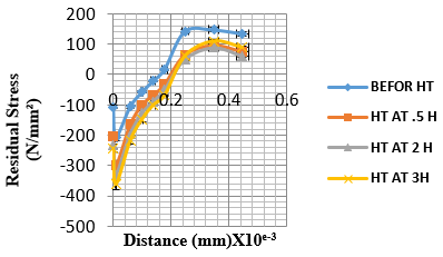
In Figure.8. show the maximum value of the residual stress is about 146.67 N/mm2 after relaxation and about 96 N/mm2 after relaxation AT 0.5 h and 50N/mm2 AT 2h. These results point out that there is a substantial effect on reducing the residual stress by applying HT with different time duration for this type of welded component [4].
Figure 7. The residual stresses before & after procedure of relaxation with different durations for x70 component
The heat treatments carried out at 550 °, 600 ° and 650 ° produce a very remarkable reduction in the residual stress value, knowing well the role of the relaxation for the improvement of the seal quality, for this steel for the best results obtained in terms of relaxation. showed to be consistent. Therefore, the results of thermal analysis obtained in this simulation were satisfactory and close to the results obtained experimentally with errors ranging from less than 5% to 13%, which are similar in range to these errors found in the literature.
|
K |
is an elastic constant for the X-ray stress measurement. |
|
M |
gradient of the data regression line representing the stress results for various angles. |
|
T |
the temperature °C |
|
k |
thermal conductivity, W.m-1. K-1 |
|
C |
is the specific heat |
|
t |
represent the heat treatment time s |
|
z |
represents the welding direction |
|
x |
in the transverse direction |
|
y |
is thickness direction. |
|
d |
is inter-planar spacing of two crystal lattices μ° |
|
Greek symbols |
|
|
ρ |
is the density g/m3 |
|
n |
is an integer |
|
θ |
is diffraction angle rad |
|
λ |
is the wavelengths 1/s |
|
e |
is the quantity of strains N/m2 |
|
θd |
is the diffraction angle in a stress free condition rad |
|
s |
The stress Mpa |
|
y |
is the angle between the sample normal and diffraction plane normal rad |
|
Subscripts |
|
|
NDT |
non destructive method testing |
|
BM |
base metal |
|
HAZ |
zone heat made |
|
ZM |
molten zone |
|
VB |
Visual Basic |
[1] American Society of Welding Website (www.aws.org).
[2] Sun WQ, Shao J, He AR, Zhao HS, Zhou J. (2015). Research on residual stress quantitative reduction in laminar cooling on hot strip mill. International Journal of Heat and Technology 33(4): 19-24. http://dx.doi.org/10.18280/ijht.330403
[3] Hamdi M. (2017). Residual stresses measurement in the weld seam of X70 Steel. Analyzed by XRD Acta Physica Polonica A 132(3-ІІ): 866-868. http://doi.org/10.12693/APhysPolA.132.866
[4] Al-olabi AG. (1994). Residual stresses and heat treatments for metallic welded components. Ph.D Theses, Dublin City University.
[5] Masubuchi K. (1983). Residual Stress and Distortion. Metals Handbook. Welding, Brazing and Soldering, ASM 6.
[6] Gür CH. (2010). Prediction of surface residual stresses in butt-welded steel plates by magnetic barkhausen noise analysis. In 10th European Conference on NDT, Moscow.
[7] Zhu XK, Chao YJ. (2002). Effects of temperature-dependent material properties on welding simulation, Computers and Structures 80: 967–976.
[8] Shiga C. (2010). Effect of Ms temperature on residual stress in welded joints of high-strength steels. Wilding in the World March 54(3-4): R71–R79. https://doi.org/10.1007/BF03263490
[9] Pamuk MT. (2018). Numerical simulation of transient heat transfer in friction-stir welding. IJHT Journal 36(1). https://doi.org/10.18280/ijht.360104
[10] Digheche K. (2017). Influence of heat treatments on the microstructure of welded Api X70 Pipeline Steel. Acta Metallurgica Slovaca 23(2): 72-78. https://doi.org/10.12776/ams.v23i1.879
[11] Benlamnouar MF. (2012). The influence of relaxation treatments on residual stresses in welded pipe API 5L-X70, METAL2012. Brno, Czech Republic, EU 5:23-25.
[12] Paddea S. (2012). Residual stress distributions in a P91 steel-pipe girth weld before and after post weld heat treatment. Materials Science and Engineering 534: 663-672. http://dx.doi.org/10.1016/j.msea.2011.12.024
[13] Boumerzoug Z. (2014). X-Ray analysis of residual stress in weld region of X70 pipeline steel. Advanced Materials Research 936: 2011-2016. https://doi.org/10.4028/www.scientific.net/AMR.936.2011
[14] Dhas JER. (2011). Weld residual stress prediction using artificial neural network and Fuzzy logic modeling. Indian Journal of Engineering & Materials Sciences 18(10): 351-360.
[15] Balasingh C, Singh AK. (2000). Residual stresses and their measurements by X-Ray diffraction methods. Metals Materids And Processes 2-3: 269-280.
[16] Gou RB. (2011). Residual stress measurement of new and in-service X70 pipelines by X-ray diffraction method. NDT & E International 44: 387–393. http://dx.doi.org/10.1016/j.ndteint.2011.03.003.
[17] Shigeru A. (2013). Probabilistic evaluation of a method for reduction of residual stress in welded structure using vibration. Chemical Engineering Transactions 33: 1087-1092. http://dx.doi.org/10.3303/CET1333182
[18] Yuan JW. (2017). Research and implementation of artificial intelligence in welding process design. Chemical Engineering Transactions 62: 649-654. http://dx.doi.org/ 10.3303/CET1762109