OPEN ACCESS
Dynamic energy simulation of buildings has recently become a very common tool to assess energy needs and thermal comfort in buildings. Software tools are now available at a low price, and allow a very detailed description of the building behaviour. However, one issue that is often neglected is the need to use accurate weather data to perform reliable dynamic simulations.
The aim of the paper is to discuss the uncertainty generated by the choice of the weather data in the energy simulation of an existing office building located in the University campus of Catania, Southern Italy. To this aim, different sets of data are considered: the first one corresponds to the weather file available in the EnergyPlus database for the airport of Catania; the second one is generated by morphing the first one with a tool that takes into account the effect of buildings, vegetation and heat sources in the urban area.
The paper discusses the differences amongst these data, and considers their impact on the calculation of the building heating and cooling load, as well as on the indoor thermal comfort. In the authors’ opinion, the outcomes of the study provide interesting information about the reliability of dynamic simulation as a tool for energy planning at urban scale. The results also point out the need to implement energy simulation with tools for weather data morphing in case of urban context.
dynamic simulations, cooling load, heating load, urban areas, weather data
In the last years, software tools for dynamic energy simulation of buildings have become commonly available and widely used in the scientific community, since they allow a detailed evaluation of the building performance, in terms of thermal loads and indoor thermal comfort.
However, reliable simulations depend strongly on the availability of accurate weather data to be used as an input for the calculation. To this aim, most of the building energy simulation tools adopt weather files based on the so-called Typical Meteorological Years (TMY). These are generated by statistically averaging long-term weather measurements, issued by weather stations commonly placed in peripheral zones, outside the urban areas [1].
Now, several drawbacks occur when using TMY as an input to dynamic energy simulation. Indeed, Wang pointed out that the actual weather data may differ significantly from the TMY referring to the same location, due to year-to-year fluctuations. This is expected to impact the calculated energy needs of a building, ranging from 5% to 10% [2]. Similar results were obtained by Pernigotto et al. who found out that even the energy rating of the building can be influenced [3].
Other authors reported important discrepancies between different weather datasets measured by different weather stations located in the same area [4]. As an example, the air temperature measured by several weather stations located in the city of Vienna were found to diverge by about 2 °C in the daytime and 4 °C at night [5]. As a consequence, the simulated annual building energy consumption is reported to show important variations (by ±7%) according to the selected weather data referring to the same area [6-7].
Another non-negligible issue is that the air temperature inside an urban context may diverge significantly from that measured by weather stations in rural areas, due to the Urban Heat Island effect [8-10]. This discrepancy can reach 3-4 °C [11], leading the cooling load of typical urban buildings to be higher (even by 13%) if compared to similar buildings in rural areas [12].
These results lead to question the suitability of the existing and universally used TMY weather datasets to accurately predict heating and cooling loads of buildings. However, the use of real weather data would require weather stations installed in the area surrounding the simulated building. This is not easy, hence such data are seldom available.
One solution to this problem might be the use of models able to modify the weather file referring to rural areas in order to make them suitable for urban areas, based on the actual urban texture. Building energy simulation tools should be connected to these models, thus allowing more efficient calculations while taking into account the impact of the microclimatic conditions on the energy demand of the building [13]. As an example, the creation of a micro-scale TMY weather file based on this approach is reported to introduce variations in the dry bulb temperature by 1–2 °C, while the predicted value of the energy consumption of a building changes by up to 11% [14].
Amongst the tools available to provide specific weather data for urban sites, the Urban Weather Generator (UWG) has recently raised particular interest. This tool estimates the local hourly air temperature and humidity in an urban site starting from weather data coming from a rural weather station. Rural weather data are first used to calculate the vertical temperature profile inside the rural canopy layer; then this is used to determine the temperature inside the urban boundary layer, and finally the temperature is projected to the urban canopy layer [15]. The process is based on the application of energy conservation principles to control volumes in the urban boundary layer and the urban canopy layer, here including the heat transfer from buildings to the urban canopy and the waste heat from air-conditioning devices [16]. UWG has low computational time, comparable to building energy simulation tools, and has been validated through a series of case studies, showing errors below 1°C in the assessment of the urban temperature if compared with measured data [17-18].
In this paper, UWG is applied to a portion of the campus of the University of Catania. Weather data generated by UWG for this area are compared with those contained in the TMY weather file for the airport of Catania, and with the data measured by a weather station operating inside the campus. The statistical analysis presented in Section 3.1 discusses the deviations amongst these different sources.
Then, the different weather data are used as an input for the dynamic simulation of a building located inside the campus, that hosts a series of offices; the results and the corresponding discrepancies are commented in Section 3.2. The aim is to test the usefulness of UWG as a tool supporting dynamic simulations, while also highlighting the importance of having reliable weather data to assess the energy performance of a building in terms of thermal load and indoor thermal comfort.
2.1 Settings for Urban Weather Generator
Figure 1 shows the portion of the University campus that is considered in this study. The campus is located north of the city center of Catania; the road delimiting the southern side of the campus is one of the busiest routes in Catania, that separates a densely built residential area from the hill hosting the University campus and the University hospital.
The area highlighted in Figure 1 has an extension of about 250 m per side, and hosts a series of buildings with offices and classrooms; the building considered for the dynamic simulations is indicated by the dashed line, and is described in detail in Section 2.2. A weather station is installed two meters above the roof of this building (which means six meters above the ground), measuring outdoor air temperature, relative humidity and global solar irradiance with a time step of 5 minutes.
Figure 1. Area included for the generation of the weather file
Starting from the TMY weather file available in the EnergyPlus database for Catania airport (Fontanarossa), UWG is able to provide a morphed weather file referring to the University campus. The output weather file is compatible with many building energy simulation programs, including Energy Plus.
To this aim, UWG needs a series of input data pertaining to the geometry of the urban area, the presence of vegetation, the traffic schedules, as well as the features of the buildings within the area. An earlier study concerning the application of UWG to Toulouse and Basel (mild climates) showed that horizontal building density (i.e. total building footprint/site area), vertical to horizontal built ratio (i.e. total façade area/site area), and vegetation coverage are the most sensitive parameters [15]. However, the role of the vegetation coverage becomes dominant only when high values occur.
The main input parameters used for this case study are listed in Table 1. The daytime and nighttime boundary layer height refers to the fact that, next to an urban settlement, the wind coming from rural areas, characterized by low roughness, meets a strong gap. An urban boundary layer develops, above which the wind keeps undisturbed features. The values of these meteorological parameters usually range between 700 m and 1000 m (daytime) or between 50 m and 80 m (nighttime), as reported in Ref. [15] and [18].
The sensible anthropogenic heat defines the amount of sensible heat released to the urban canopy by anthropogenic activities, and includes all contributions such as traffic, street lighting and human metabolism. The sensible heat released by buildings and air-conditioning devices is not included in this parameter, and is calculated by a specific algorithm in UWG. The average building height, vertical to horizontal built ratio and horizontal building density have been estimated by means of satellite images and in-field observations. The estimated road albedo is 0.2. The building type parameter is 100% of large offices.
The vegetation albedo is set to 0.25, which is the average value reported in the literature [15]. The model accounts for the effect of vegetation from January to December (evergreen vegetation). The vegetation coverage has been estimated from satellite images.
However, in order to analyze the effects of the main input parameters on the air temperature profile, several simulations were carried out where, starting from the input parameter listed in Table 1, the following variations were considered:
(1) sensible anthropogenic heat: 10 W/m2;
(2) building type: 50% offices + 50% secondary schools;
(3) vegetation coverage: 0;
(4) road albedo: 0.1.
2.2 Dynamic energy simulations of the selected building
The building selected as a case study is an office building that hosts, at the upper floor, some offices and a meeting room, while the basement is occupied by laboratories. The main façade is oriented to north (Figure 2).
The outside walls are made of a double leaf of concrete blocks (120 mm) and hollow clay blocks (80 mm), separated by an air gap containing a thin layer of polystyrene (30 mm). The outer surface is covered by a basalt sheet, whose solar reflectance has been set to 0.3. The resulting thermal transmittance is U = 0.66 W·m-2·K-1.
The roof is made of a prefabricated concrete structure covered by a layer of mineral wool (30 mm) and a lightened cement screed (100 mm). The top layer of clay shingles (12 mm) is placed over a 20-mm cement screed; on the inner side, a plasterboard (20 mm) covers a small air gap (30 mm) underlying the prefabricated structure. The thermal transmittance of the roof is U = 0.72 W·m-2·K-1, while the solar reflectance of the top layer is 0.25.
Table 1. Key settings for UWG simulation
|
Parameter |
Setting |
|
Daytime boundary layer height |
1000 m |
|
Nighttime boundary layer height |
50 m |
|
Average building height |
7.83 m |
|
Vertical to horizontal built ratio |
0.30 m2/m2 |
|
Horizontal building density |
0.27 m2/m2 |
|
Sensible anthropogenic heat |
5 W/m2 |
|
Road albedo |
0.2 |
|
Albedo of vegetation |
0.25 |
|
Begin month for vegetation |
January |
|
End month for vegetation |
December |
|
Vegetation coverage |
0.06 |
|
Latent fraction of vegetation |
0.5 |
|
Building type |
100% large offices |
The window to wall ratio is WWR = 46%, meaning that the window surface has a significant role on the thermal performance of the building. The ratio of the overall envelope surface to the gross volume of the building is S/V = 0.47 m-1. The neighboring buildings are sufficiently far, so as not to cast shadows on the roof of the sample building.
Figure 2. Main façade of the selected building (facing north)
Figure 3. Plan of the selected building
The dynamic thermal performance of the building has been simulated through EnergyPlus 8.4 [19]. In order to simplify the simulations, only a part of the building was modeled, including the offices shown in Figure 3. The other offices located in the east wing of the building were not included in the model; however, the right-hand boundary of Figure 3 was simulated as an adiabatic surface, to take into account that on that side there are other indoor spaces with a temperature close to that reached in the simulated spaces. The entrance hall has a temperature calculated as the average between the outdoor temperature and the temperature of Office 1: this can be regarded as a good approximation, taking into account that the entrance door is very frequently kept open and that the hall is highly ventilated.
In the simulations, the building is set as occupied from 09:00 to 18:00 during weekdays, and shows internal gains due to people activity, electric equipment and artificial lighting. In particular, each office is constantly occupied by one person carrying out typical office tasks, and releases 120 W of sensible heat; in the assembly room six people are considered, but only occasionally from 09:00 to 12:00. The internal loads for artificial lighting are 5 W/m2, usually switched on in the afternoon. The heat gains due to electric equipment are 150 W per room.
The air infiltration rate is set constant to 0.3 h-1 throughout the day. Additionally, a natural ventilation rate is also considered to account for the intentional windows opening; according to the habits of the occupants, a small ventilation rate is considered in winter (0.3 h-1), but in summer this value is increased to 2 h-1. However, such additional ventilation rate is excluded when the outdoor temperature is too hot in summer (above 32 °C) or too cold in winter (below 14 °C).
When the simulation is performed under thermostatic control, the set point temperature for the air-conditioning system is 26 °C in summer and 20 °C in winter, but only during the office hours.
3.1 Weather data
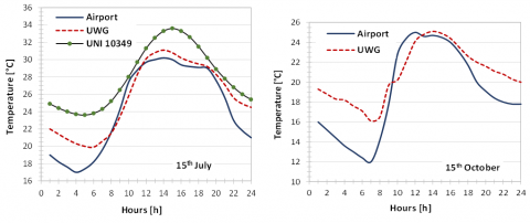
Figure 4 compares the hourly values of the outdoor air temperature calculated by UWG and those available in the TMY weather file for Catania airport (Fontanarossa). In order to simplify the discussion, only the results of the 15th of January, April, July and October are reported.
Now, from the sensitivity analysis performed for the main input parameters in UWG (sensible anthropogenic heat, building type, vegetation coverage, road albedo), no significant variation of the output was observed. In fact, it was found that the maximum variation of the hourly temperature generated for the University campus does not exceed 0.1 °C (when no vegetation is considered). This confirms what already observed in other studies, where building density and vertical to horizontal built ratio turned out to be the most sensitive parameters [15, 18]. For this reason, just one UWG profile is reported in the following.
From the observation of Figure 4, it is clear that urban air temperatures are generally higher than in rural areas, such as near the airport. The discrepancy between the two profiles can be small or even negligible during the central part of the day, especially in January; on the other hand, it gets more intense at night, especially in July and October. This is due to the fact that common building materials have higher heat capacity than vegetation and soil: this implies that streets, buildings and parking lots tend to retain thermal energy longer, thus keeping warmer than surrounding rural areas, and then releasing heat at night.
Figure 4 also includes the design summer temperature profile for Catania, according to UNI 10349-2 [20]. This is the temperature profile to be used when assessing the cooling load in summer, and refers to an average hot day in July.
Figure 5 shows a further comparison between Fontanarossa and UWG weather data. In particular, for each month of the year the graph correlates the minimum, maximum and mean outdoor air temperature for both weather data. Here again, it is found out that the UWG value is almost always higher than for the airport, and that the highest discrepancy refers to the monthly minimum temperature; in December, this even attains 5°C. On the other hand, the discrepancy between the monthly maximum outdoor temperature is less evident, and hardly exceeds 1°C. In November and December, the maximum outdoor temperature is unexpectedly slightly higher in the urban context than for the airport. Finally, from Figure 5 it is possible to notice that the mean value of the outdoor air temperature provided by UWG is always higher than for the airport, and that the difference ranges between 0.8°C and 1.5°C, the highest values occurring in summer.
A further result is shown in Figure 6, which plots the cumulated distribution of the outdoor air temperature in July and August. In this case, the comparison also includes the data measured in the summer 2017 by the weather station inside the campus, on top of the building used as a case study.
From this analysis it comes to light that the actual outdoor air temperature recorded in-field by the weather station is even higher than what is predicted by UWG. As an example, according to the recorded data the outdoor air temperature exceeds 30°C for about 29% of time, whereas this happens for 16% of time according to UWG, and for only 10% of time at the airport. Moreover, the recorded values exceed 33°C for about 11.5% of time, while this occurs rarely if looking at Fontanarossa or at the UWG results. Finally, the maximum recorded value in the summer 2017 is 41.1°C, i.e. 5.5°C above the maximum value proposed by UWG.
However, it is important to underline that the UWG results, being derived by morphing the TMY weather file of the airport, have statistical significance over a long period of time (e.g. 30 years), and cannot be directly compared with data referring to a short period of time (in this case, July and August 2017), when anomalous events may have occurred. Moreover, the data were recorded by the weather station at the height of about six meters above the ground, while TMY data refer to the height of two meters above the ground.
In any case, as already highlighted in other studies, it is possible to conclude that the TMY weather data normally used for building energy simulations underestimate the actual urban temperatures. The mean error with respect to the UWG data is, in this case, in the range of about 1÷1.5°C, but can exceed 4° C in some moments of the day.
Figure 4. Comparison of the outdoor air temperature profiles
Figure 5. Monthly analysis of the outdoor air temperature
Figure 6. Air temperature: Cumulated distribution in summer
3.2 Results of the dynamic simulations
The different weather data discussed in Section 3.1 are then used as an input for the dynamic simulation of the office building shown in Section 2.2. The aim is to investigate the sensitivity of the results to the variation of the weather data due to the specific urban context; in particular, the building performance is evaluated through the space heating and cooling load under thermostatic control, while also looking at the time profile of the indoor operative temperature in a particularly hot week in summer.
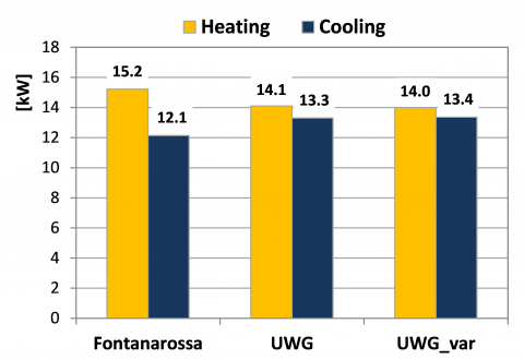
Figure 7 shows the seasonal thermal energy needs of the building for space heating and cooling, referred to the unit floor surface. The graph compares the results obtained by using respectively the TMY weather file available for Fontanarossa airport and the weather file generated by UWG for the University campus. In this last case, two different versions are considered, associated respectively to the basic settings discussed in Section 2.1 and to one of the variants proposed during the sensitivity analysis (no vegetation), which however turned out to introduce only slight variations on the outdoor air temperature. As a consequence, the sensitivity of the heating and cooling loads to the different proposed settings of UWG is almost negligible.
As expected, the use of UWG weather data causes for the selected building higher space cooling needs than with the weather data referred to the airport. The difference amounts to 13.4%, with only slight deviations between the different versions of the UWG simulation. On the other hand, in winter the building can take advantage of the higher outdoor air temperature, and the space heating needs are significantly reduced (-13.6%). Overall, in this case the annual total energy needs are only slightly increased.
Figure 7. Effect of the weather file on heating/cooling needs
Figure 8. Effect of the weather file on the peak load
Figure 9. Operative temperature for two rooms in August
Similarly, Figure 8 compares the results in terms of peak heating and cooling load. In this case, UWG data increase the peak cooling load by around 10%, while also reducing the peak heating load by around 7%.
Finally, Figure 9 allows to measure the effect of the different weather datasets in terms of indoor operative temperature, obtained by dynamic simulations in free-running conditions. The results refer to a particularly hot week in summer (from 17th to 22nd of August) and to two representative rooms (see Figure 3). All the other rooms show an intermediate behaviour.
As observed, the use of UWG data generates significant increases in the simulated indoor operative temperatures, especially in Office 6, where the overheating ranges between 0.9°C and 1.2°C.
The results of this paper show the importance of using reliable weather data when performing the dynamic energy simulation of buildings located in an urban context. To this aim, researchers can rely on tools able to morph the TMY weather files available for rural areas, and to adapt them to the specific urban texture, such as Urban Weather Generator.
In this study, the use of UWG in relation to a portion of the University campus of Catania, in Southern Italy, has produced a general increase in the outdoor air temperature, if compared to the values reported in the TMY weather file available for Catania airport. The mean discrepancy ranges around 1÷1.5°C, but it can exceed 4° C at night in summer.
Now, the results of UWG depend on a series of settings, such as the geometry of the urban site, the presence of vegetation, the rate of anthropogenic heat and the features of the buildings within the area. For this reason, a sensitivity analysis has been performed, but the results did not vary significantly by changing the sensible anthropogenic heat, the building typology, the vegetation coverage and the road albedo. Actually, the vegetation coverage is a very sensitive parameter according to the literature; however, in this case it was already very low (6%), hence setting it at zero produced only slight variations (0.1 °C on the peak temperature).
The consequence of a different outdoor temperature on the energy performance of a building is not negligible. With reference to the selected office building in the University campus, the energy needs for heating and cooling changed by around 13.5 % if compared to a simulation performed with the airport weather data. On the other hand, the predicted indoor operative temperature in free running conditions may diverge by 0.9 ÷ 1.2 °C. These results refer to an office building with average insulation levels, and might be different for other destinations or in case of better insulation.
Future studies will aim to apply the same procedure to other sites, and in particular to residential buildings located in the city center of Catania. Here, the presence of urban canyons, the absence of vegetation and the very high anthropogenic heat rates are likely to produce an intense Urban Heat Island effect. This is usually overlooked in dynamic simulations, but it can be now effectively included by means of Urban Weather Generator.
[1] Tsoka S, Tolika K, Theodosiou T, Tsikaloudaki K, Bikas D. (2018). A method to account for the urban microclimate on the creation of typical weather year datasets for building energy simulation, using stochastically generated data. Energy Build 165: 270–283. https://doi.org/10.1016/j.enbuild.2018.01.016
[2] Wang L, Mathew P, Pang X. (2012). Uncertainties in energy consumption introduced by building operations and weather for a medium-size office building. Energy Build 53: 152–158. https://doi.org/10.1016/j.enbuild.2012.06.017
[3] Pernigotto G, Prada A, Cóstola D, Gasparella A, Hensen JLM. (2014). Multi-year and reference year weather data for building energy labelling in north Italy climates. Energy Build 72: 62–72. https://doi.org/10.1016/j.enbuild.2013.12.012
[4] Pyrgou VL, Castaldo A, Pisello L, Cotana F, Santamouris M. (2017). Differentiating responses of weather files and local climate change to explain variations in building thermal-energy performance simulations. Solar Energy 153: 224–237. https://doi.org/10.1016/j.solener.2017.05.040
[5] Vuckovic M, Kiesel K, Mahdavi A. (2016). Toward advanced representations of the urban microclimate in building performance simulation. Sustain Cities Soc 27: 356–366. https://doi.org/10.1016/j.scs.2016.05.002
[6] Bhandari M, Shrestha S, New J. (2012). Evaluation of weather datasets for building energy simulation. Energy Build 49: 109–118. https://doi.org/10.1016/j.enbuild.2012.01.033
[7] Erba S, Causone F, Armani R. (2017). The effect of weather datasets on building energy simulation outputs. Energy Procedia 134: 545–554. https://doi.org/10.1016/j.egypro.2017.09.561
[8] Pyrgou V, Castaldo L, Pisello AL, Cotana F, Santamouris M. (2017). On the effect of summer heatwaves and urban overheating on building thermal-energy performance in central Italy. Sustain Cities Soc. 28: 187–200. https://doi.org/10.1016/j.scs.2016.09.012
[9] Sheikhi A, Kanniah KD. (2018). Impact of land cover change on urban surface temperature in Iskandar Malaysia. CET 63(25). https://doi.org/10.3303/CET1863005
[10] Kanniah KD, Siong HC. (2017). Urban forest cover change and sustainability of Malaysian cities. CET 56. https://doi.org/10.3303/CET1756113
[11] Gobakis K, Kolokotsa D. (2017). Coupling building energy simulation software with microclimatic simulation for the evaluation of the impact of urban outdoor conditions on the energy consumption and indoor environmental quality. Energy Build 157: 101–115. https://doi.org/10.1016/j.enbuild.2017.02.020
[12] Liu Y, Stouffs R, Tablada A, Wong NH, Zhang J. (2017). Comparing micro-scale weather data to building energy consumption in Singapore. Energy Build 152: 776–791. https://doi.org/10.1016/j.enbuild.2016.11.019
[13] Bueno L, Norford J, Hidalgo GP. (2012). The urban weather generator. J Build Perform Simul 6(4): 269-281. https://doi.org/10.1080/19401493.2012.718797
[14] Bueno L, Norford GP, Britter R. (2012). A resistance-capacitance network model for the analysis of the interactions between the energy performance of buildings and the urban climate. Build Environ 54: 116-125. https://doi.org/10.1016/j.buildenv.2012.01.023
[15] Nakano B, Bueno LN, Reinhart CF. (2015). Urban Weather Generator – a novel workflow for integrating urban heat island effect within urban design process. In Proc. 14th IBPSA Conference, pp. 1901–1908.
[16] Bueno M, Norford RL, Li R. (2014). Computationally efficient prediction of canopy level urban air temperature at the neighbourhood scale. Urban Clim 9: 35–53. https://doi.org/10.1016/j.uclim.2014.05.005
[17] Nakano A, Bueno B, Norford L, Reinhart CF. (2015). Urban Weather Generator – a novel workflow for integrating urban heat island effect within urban design process. In Proc. 14th IBPSA Conference, pp. 1901–1908.
[18] Bueno B, Roth M, Norford L, Li R. (2014). Computationally efficient prediction of canopy level urban air temperature at the neighbourhood scale. Urban Clim 9: 35–53. https://doi.org/10.1016/j.uclim.2014.05.005.
[19] US Department of Energy. (2016). Energy Plus version 8.4. https://energyplus.net/
[20] UNI 10349-2 (2016). Riscaldamento e raffrescamento degli edifici - Dati climatici - Parte 2: Dati di progetto., Italy.