OPEN ACCESS
Natural circulation is the most important heat removal mechanism for passive protection systems in a lot of industrial applications, such as nuclear power plants, solar energy systems, reboilers and cooling of electronic systems. The aim of the present work is to investigate the flow and heat transfer characteristics of parallel loops, connected in the lower heated sections, in single-phase natural circulation.
The test facility was composed by 2 vertical circuits connected in parallel; each of them was rectangular in geometry, the aspect ratio (defined as the height to width ratio) was 1.63, with circular copper tube of 4 mm (I.D.). An upper cold heat exchanger provided the heat sink, while the heat source at the bottom was a power supply system. Several calibrated thermocouples (T-type) placed in the fluid along the vertical tubes allowed the evaluation of the hot and cold legs average fluid temperature differences.
Tests were carried out imposing 3 different heat sink temperatures (10, 20, 30°C); for each of these temperatures the power supply at the lower heater was increased from 20 to 90 W. The fluid investigated was distillate water.
The experimental results have been analysed in terms of thermal performance of the single or connected loops. Collected data have also been compared with Vijaiyan’s correlation
Single-phase natural circulation loop, parallel circuits, different heat sink temperature
Natural convection flow in loops has been thoroughly investigated over the past four decades. The several fields of interest cover applications such as cooling of electronic circuity, nuclear applications, material processing, geothermal energy extraction, environmental processes, storage systems, passive safety systems, etc.
Natural circulation of a fluid occurs in presence of temperature and density gradients in a force field, like gravity, due to a heat source and a heat sink in thermal contact with the fluid that establish and maintain circulation with no need of external mechanical moving aid.
There is no general way to predict the distribution of the thermo-hydraulic behaviour and the loop performance. In fact many variables act together such as the following geometric factors:
Hydraulic diameter of the tubes;
Aspect ratio (H/W, height/length) of the loop;
Orientation of the loop;
Heat source and heat sink displacements (horizontal, vertical).
From the operating point of view the following variables play a fundamental role on the thermal-hydrodynamic behaviour of a natural circulation loop:
Fluid characteristics;
Heater and heat sink locations;
Heat sink temperature;
Heater power input.
The dynamic natural circulation behaviour was experimentally and numerically investigated. The first studies were carried out by Keller [1] and Welander [2]. More recently Chen [3], Vijayan et al. [4-5], Misale et al. [6], Devia and Misale [7], Misale [8] and Swapnalee and Vijayan [9] developed theoretical analyses in order to focus the influence of the loop geometrical characteristics on the natural circulation instabilities.
Natural circulation loops (NCLs) investigated in literature are usually single-phase vertical rectangular or toroidal loops, with simply geometrical shapes. Only few works are focused on complex loops, with additional connecting pipes or more coolers/heaters. Satoh et al. [10] studied the influence of a upper double cooler by means of a numerical approach, while the Authors [11] experimentally analysed the influence of a connecting tube between the half lower heated slice and the upper one (cooled section).
In this context our attention is focused on experimental works. In particular this paper deals with an improvement in phenomena observation. A summary of the works relevant to the experimental investigations regarding rectangular systems is reported in Tab. 1, where the description of loop configuration, the instrumentations used, the major geometrical dimensions and the operating conditions are mentioned.
The aim of this study is to experimentally investigate two natural circulation loops connected at the heated section.
The experimental setup is depicted in Fig.1, whereas in Tab.2 are reported the geometrical dimension of each rectangular loop. The apparatus consists of two rectangular vertical loops connected in the bottom side by two tubes made of copper. Each rectangular loop utilises copper tubes for horizontal and vertical parts of the loop. The four curves are made with silicon tubes. The internal diameter of the circular cross section is 4 mm, whereas the thickness of the tube is 2 mm. The same tube is used to connect the two rectangular loops. The distance between the two parallel loops is 120 mm. The flow in the circuit is induced by the presence of a heater in the bottom side of the loop and a cooler at the top part of the loop. The heater is realised by a nicromel wire rolled around the horizontal tube, whereas the heat sink is a coaxial heat exchanger located at the top side of the loop. The temperature at the heat sink is controlled by a cryostat (Haake F3, temperature stability ±0.1°C). In order to increase the flow rate of the secondary flow, an external circulator (Calpeda CAM 60E) is used which guarantee a flow rate higher than 10 l/min. This high value of flow causes a constant temperature in the external side of the heat sink. The thermal boundary conditions are: imposed heat flux at the heater and imposed temperature at the cooler.
Figure 1. Experimental setup (dimensions in mm)
The fluid temperature are measured by six T-type shielded/calibrated thermocouples (O.D. of 0.5 mm/±0.1 K), whereas two additional thermocouples are used to measure both the ambient temperature and the secondary fluid temperature (50% water, 50% glycol) in the cryostat bath. Six calibrated sheathed thermocouples (±0.1°C) are located in the vertical legs of the loop and the hot junction of each thermocouple is placed in the middle of the cross section at the distance from the heater reported in Fig. 1. The presence of a small part of the thermocouple wire in the cross section of the tube reduce it of 7.9%. This value is sufficiently small to neglect the consequent increment of pressure loss.
The temperature data are acquired and stored by a National Instruments data acquisition system (SCXI 1102, SCXI 1303, SCXI 1000, PCI-1200). The frequency sampling is 1 s, with a minimum test duration of 10000 s.
Each run started from stagnant condition of the working fluid. The following procedure was applied to each run: prepare the cryostat at the desiderate temperature and at the same time switch on the power supply and open the valve that put in connection the cryostat with the heat sink.
To better investigate the mutual influence of the two connected loops a first series of test was performed increasing and decreasing the power in case of no-connecting loops. The data allowed to know the thermal performance of each loop when the secondary fluid temperature was selected by the cryostat (10, 20 and 30°C).
A second series of test was performed in case of connected loops. In particular, two different procedures were used:
Procedure A): The same range power (20 W-90 W, power step of 10W) was supply to loops #1 and 2 during the increasing and decreasing phases.
Procedure B): A constant power of 40 W was applied at loop #2, whereas the loop#1 started the power from 20 W up to 90 W with power step of 10 W. The power to loop #1 was applied increasing and decreasing with the same step power
Tables 3,4 and 5 report the operative conditions tested for each procedure.
The data collected during the different runs are analysed in terms of absolute values of the average temperature difference between hot and cold legs (several runs move clockwise and other runs move counterclockwise):
Table 1. Experimental studies on rectangular natural circulation loops.
|
Ref. |
Fluid |
Loop configuration |
Instrumentation |
Diameter [mm]/ Aspect ratio (H/D)/ Inclination [deg] |
Power [W] |
Heat sink temp. [°C] |
|
Misale et al. [13] |
Distilled water / Al2O3 nanofluid |
Rectangular, copper tubes, heater: horizontal bottom; heat sink: horizontal at the top. |
K-type TC |
4/ 1.47/0-30-60-78 |
10-30-50 |
10-20-30-40 |
|
Pilkhwal at al. [14] |
Water |
Rectangular, glass tubes, the loop is equipped with vertical and horizontal heaters and coolers thus obtaining different working configurations. |
K-type TC |
26.9/ 1.55/ 0 |
100÷800 Step 100 |
Ambient tap water |
|
Kudariyawar et al. [15] |
Water |
Rectangular, copper tubes, the loop is equipped with horizontal heaters, vertical horizontal coolers, thus obtaining different working configurations. |
3D simulation |
26.9/ 1.55/ 0 |
90-105-120-135-196-220-257-450 |
Ambient tap water |
|
Venkatesh et al. [16] |
Water |
Rectangular, copper tubes, heater: horizontal bottom; heat sink: horizontal at the top. |
|
8.5/ 1.51/ 0 |
50÷450 Step 50 |
30 |
|
Garibaldi and Misale [17] |
FC 43, Water |
Rectangular, copper tubes, heater: horizontal bottom; heat sink: horizontal at the top. |
K-type and T-type TC |
4/ 0.83/ 0-30-75 |
2.5-5-7.5-10-15-20-30-50 |
0 |
|
Doganay and Turgut [12] |
De-ionized water with different concentration and size (10-30nm) of Al2O3 nanofluid. |
Rectangular, copper tubes, heater: horizontal bottom; heat sink: horizontal at the top. |
K-type TC |
4.75/ 1.38/ 0-30-60-75 |
10-20-30-40-50 |
10-20 |
|
Misale el al. [6] |
Distilled water and nanofluid Al2O3 with 2 different concentration. |
Rectangular, copper tubes, heater: horizontal bottom; heat sink: horizontal at the top. (miniloop) |
T-type TC |
4/ 1.47/ 0-30-60-75 |
10-30-50 |
10-20-30-40 |
|
Vijayan et al. [5] |
Water |
Rectangular, copper tubes, the loop is equipped with horizontal heaters, vertical horizontal coolers, thus obtaining different working configurations. |
K-type TC |
26.9 / 1.49/0 |
<270 |
30 |
|
Luzzi et al. [18] |
Water |
Rectangular, copper tubes, heater: horizontal bottom; heat sink: horizontal at the top. |
K-type TC |
30/ 0.88/ 0 |
2000 |
4-5-7-8-9-10-11-14-18 |
|
Kudariyawar et al. [19] |
Molten salts (NaNO3 and KNO3, 60:40) |
Rectangular; heat sink: horizontal at the top; heater: vertical arm at the bottom. |
K-type TC |
13.88/ 1.43/ 0 |
1200÷2000 Step 100 |
Ambient tap water |
|
Gorman et al. [20] |
Water |
Circular glass loop, heat sink on the top, heater at the bottom. |
Thermistor |
Toroidal 2.1 / R=38 / 0 |
|
31 |
|
Mousavian et al. [21] |
Water |
Rectangular, copper tubes, heater: horizontal bottom; heat sink: horizontal at the top. |
K-type TC |
40 / 0.84 / 0 |
500÷1000 step 100 |
30 |
|
Suda [22] |
Water |
Rectangular, Pyrex glass tube, heater: horizontal bottom; heat sink: horizontal at the top. |
K-type TC |
30 / 1.05 / 0 |
0÷1200 |
23 |
|
Huang and Zelaya [23]
|
Water |
Rectangular, copper tubes, heater: vertical on the left arm; heat sink: vertical on the right arm. |
T-type TC |
2.8 / 2 / 0 |
225÷1400 |
Ambient tap water |
$\Delta T_{a v g}=\left|\overline{T_{h}}-\overline{{T}_{c}}\right|$ (1)
where $\overline{T_{h}}$ and $\overline{{T}_{c}}$ are the average of the hot and cold leg temperatures.
Moreover, the average fluid velocity was calculated on the basis of heat balance at the heater.
$\overline{W}=\frac{P}{A \cdot \rho \cdot c \cdot \Delta T_{a v g}}$ (2)
4.1 No connected loop #1
As reported above, a first series of tests was performed in case of no connected loop. Since the thermal performance of the two single loops (#1 and #2) are quite the same (maximum difference of ∆Tavg equal to 0.3 °C), Loop #1 is considered as reference one.
Table 2. Loop dimensions (mm)
|
Width (W) |
600 |
|
Height (H) |
970 |
|
Internal tube diameter (D) |
4 |
|
Heated length |
380 |
|
Cooled length |
420 |
|
Total length (Lt) |
2780 |
|
Ratio Lt/W |
3475 |
|
Ratio H/W |
1.62 |
|
Horizontal connecting internal diameter tube Dc |
4 |
|
Horizontal connecting tube length Lc |
120 |
|
Ratio Lc/Dc |
30 |
Figure 2 shows the average temperature differences between hot and cold legs of circuit #1 (Figure 2a) and average fluid velocity (Figure 2b) as function of both power input (20÷90 W) and heat sink temperature (10, 20, 30°C). Each curve depicted average value of data collected during the repeatability tests. The maximum deviation from the average value drawn in Figure 2a/b are ±0.2 °C and ±0.1 cm/s, respectively.
Table 3. Tests operative conditions: Circuits #1 and #2, no connected loop
|
Theat sink [°C] |
||||
|
10 |
20 |
30 |
||
|
Power #1 [W] step 10 |
from 20 |
|
|
|
|---|---|---|---|---|
|
|
|
|
||
|
to 90 |
|
|
|
|
|
Theat sink [°C] |
||||
|
10 |
20 |
30 |
||
|
Power #1, #2 [W] step 10 |
from 20 |
|
|
|
|---|---|---|---|---|
|
|
|
|
||
|
to 90 |
|
|
|
|
|
|
Theat sink [°C] |
|||
|
10 |
20 |
30 |
||
|
Power #1 [W] step 10 |
from 20 |
|
|
|
|---|---|---|---|---|
|
|
|
|
||
|
to 90 |
|
|
|
|
Moreover, it is clear the influence of the heat sink temperature: when it increases, the average difference temperature decreases for a fixed heat power dissipated at the heater [24-27].
4.2 Connected loops
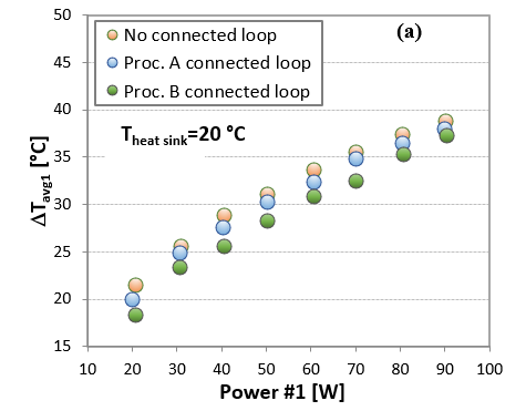
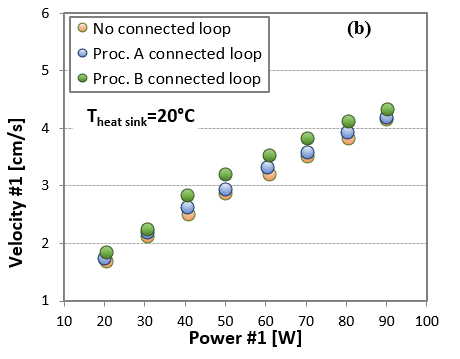
As reported in the introduction, the main target of this paper is the natural circulation in a connected parallel rectangular loops. Two different operating procedures are adopted, as described in the previous section 3. Loop #1 results adopting Procedures A and B are compared with the data collected in case of no-connected loop #1. In particular, it is interesting to analyse the influence of the parallel connected circuit #2 on circuit #1 behaviour, when the power inputs of the two loops are equal (procedure A) or the power supply of loop #2 is fixed to 40 W (procedure B).
Figure 3 shows details of the 3 procedures for Theat sink=20°C. Procedure B behaves the lowest temperature differences, (Figure 3a) while the condition with no-connected loop #1 achieves the highest values for all heat sink temperatures.
Probably the connecting tube allows that a small amount of fluid (“fresh liquid”) of loop #2 participates at the heat transfer of loop #1 reducing the average temperature difference.
Opposite behaviours are presented in Figure 3b, which reports the circuit #1 fluid velocities versus circuit #1 power input, for all the operative conditions investigated: highest velocities are exhibited for and for Procedure B. Similar trends are found for the other heat sink temperatures (10°C and 30°C).
4.3 Data reduction analysis
Figure 3. Behaviour of the circuit #1 average difference temperature (a) and velocity (b) versus heat power of circuit #1
Figure 4. Behaviour of the circuit #1 averaged difference temperature in terms of thermophysical, geometrical and operative conditions.
The influence of the fluid thermosphysical properties on the average temperature difference could be analysed by means of Bernoulli’s equation applied in case of laminar flow and heat balance. If the wall frictional stress could be neglected for velocity evaluation, the buoyancy and tangential wall forces balance leads to the relationship (3) among the average temperature difference and fluid thermosphysical properties (k, c, b, r, Pr), geometrical (height H, length L, internal diameter D) and operative conditions (power input P):
$\Delta T_{a v g} \propto \sqrt{\frac{128 \cdot P \cdot L / D}{\pi \cdot D^{3} \cdot H \cdot g}} \cdot \sqrt{\frac{k}{(c \cdot \rho)^{2} \cdot \beta} \cdot P r}$ (3)
Figure 4 reports the experimental ∆Tavg values of circuit #1 in terms of Equation (3). The trend is linear.
As suggested by Vijayan, the steady-state data could be evaluated by means of an analytical correlation: in case of stable flow, the gravitational forces balance the shear stresses and the steady state Reynolds number Ress could be correlated with a modified Grashof number Grm, heat flux, geometry and mean fluid temperature:
$R e_{S S}=\frac{\overline{w} \cdot D}{v}$ (4)
$G r_{m}=\frac{D^{3} \cdot \rho^{2} \cdot P \cdot H}{A \cdot \mu^{3} \cdot c} \cdot \beta \cdot g$ (5)
The final correlations are:
$R e_{s s}=0.1768 \cdot\left[\frac{G r_{m}}{N_{G}}\right]^{0.5}$ for laminar flow (6)
$R e_{s s}=1.96 \cdot\left[\frac{G r_{m}}{N_{G}}\right]^{0.364}$ for turbolent flow (7)
NG is a geometrical parameter calculated in terms of the ratio between the total length and the internal diameter of the loop, and the ratio between concentrated and uniform pressure losses:
$N_{G}=\left(\frac{L_{t o t}}{D}+\frac{k}{f}\right)$ (8)
Figure 5. Steady state natural circulation data.
where f=64/Ress and k was evaluated with Idelchik (1994).
The Ress experimental data of all the runs are depicted in Figure 5 versus (Grm/NG) and compared with laminar flow Vijayan correlation.
Experimental data seem to be well correlated by the analytical correlation, with a underestimation for the lower Grm/NG values.
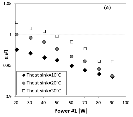
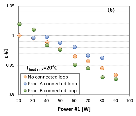
Figure 6 reports the circuit #1 effectiveness reported in terms of power input #1 (10÷90 W).
Effectiveness refers to the ratio of actual heat transfer to maximum possible one; it has been evaluated as follows:
$\varepsilon=\frac{\Delta T_{a v g}}{T_{h}-T_{h e a t \sin k}}$ (9)
In equation (9) Th represents the inlet liquid temperature in the heat sink, assumed equal to the left leg mean temperature if the fluid flow is clockwise, and equal to the right leg mean temperature if the fluid flow is counterclockwise.
In Figure 6a the no-connected loop behaviour is showed for the 3 different heat sink temperatures investigated.
The best performance in terms of average difference temperature (Figure 2a) is achieved for Theat sink=30°C, whereas in terms of efficiency for this heat sink temperature it shows the lowest performance even though all values of efficiency varying in a reduced spread (between 1 and 0.96).
In Figure 6b the efficiency for both no-connected and connected loop are depicted for the different operating procedures adopted during the experiments (no-connected loop; Procedure A; Procedure B), at Theat sink=20°C.
For all the heat sink temperatures investigated Procedure A leaded to highest values of efficiency. These results suggest that the average difference temperature is not the only parameter to take in account for the evaluation of the system thermal performance (the minimum values of the average difference temperatures were found for Procedure B): a more thorough analysis could be extended to other thermosphysical and geometrical parameters, including the horizontal connecting leg influence on the loop mutual link.
Figure 6. Efficiency of circuit #1 versus power input.
In the present paper an experimental investigation on single-phase natural circulation loops was presented. A first step of the work has been focused on a single loop, in which the upper horizontal section was cooled by a heat sink (cryostat) and the lower one by a heater. The average difference temperature between the two vertical legs was analysed for different heat sink temperatures and heater power input.
Afterwards the investigation was focused of the mutual influence of two connected loops, which have been heated following two different procedures, with the power inputs of the two loops equal (procedure A) or the power of loop #2 fixed to 40 W and varying the power of loop #1 (procedure B).
Then experimental average temperature difference data were analysed for underline the influence of the fluid thermosphysical properties. The results are very interesting and suggest a correlation between the temperature difference and a proper combination of thermosphysical properties and operative conditions.
For all the heat sink temperatures investigated, loop #1 showed the lowest temperature difference at the heated section in case of connected loop (Procedure B) whereas it achieves the highest values for no-connected loop.
Experimental data have been compared with the analytical correlation proposed by Vijayan, showing a good agreement.
In terms of effectiveness, the best perform of no-connected loop is achieved for the highest heat sink temperature, while for all the heat sink temperatures investigated Procedure A leaded to highest values of efficiency.
|
A |
Internal cross section area [m2] |
|
c |
Water specific heat [J/kgK] |
|
D |
Internal tube diameter [m] |
|
Dc |
Horizontal connecting internal diameter [m] |
|
f |
Friction factor (64/Ress) |
|
Grm |
Modified Grashof number [-] |
|
H |
Circuit Height [m] |
|
k |
Concentrated pressure losses coefficient |
|
Lc |
Horizontal connecting pipe length [m] |
|
Lt |
Circuit total length [m] |
|
NG |
Concentrated and uniform pressure losses parameter |
|
P |
Power input [W] |
|
Pr |
Prandtl number [-] |
|
Ress |
Steady state Reynolds number |
|
Theat sink |
Heat sink temperature [°C] |
|
$\overline{{T}_{h}}$ |
Average hot leg temperature [°C] |
|
$\overline{{T}_{c}}$ |
Average cold leg temperature [°C] |
|
W |
Circuit width [m] |
|
b |
coefficient of thermal expansion [1/K] |
|
ε |
Effectiveness factor [-] |
|
μ |
Dynamic viscosity [kg/ms] |
|
ρ |
Water density [kg/m3] |
[1] Keller JB. (1966). Periodic oscillations in a model of thermal convection. J. Fluid Mech 1(26): 599-606.
[2] Welander P. (1967). On the oscillatory instability of a differentially heated fluid loop. J. Fluid MEch 29: 17-30.
[3] Chen K. (1985). On the instability of closed-loop thermosiphons. J. Heat Transf 107: 826-832.
[4] Vijayan PK, Austregesilo H, Teschendorff V. (1995). Simulation of the unstable oscillatory behaviour of single phase natural circulation with repetitive flow reversals in a rectangular loop using the computer code ATHLET. Nucl. Eng. Des 155: 614-623.
[5] Vijayan PK, Sharma M, Saha D. (2007). Steady state and stbility characteristic of single-phase natural circulation in a rectangular loop with different heater and cooler orientations. Experimental Thermal and Fluid Science 31: 925-945.
[6] Misale M, Ruffino P, Frogheri M. (2000). The influence of the wall thermal capacity and axial conduction over a single-phase natural circulation loop: 2-D numerical study. Heat Mass Transf 36: 533-539.
[7] Devia F, Misale M. (2012). Analysis of the effects of heat sink temperature on single-phase natural circulation loops behaviour. International Journal of Thermal Sciences 59: 195-202.
[8] Misale M. (2016). Experimental study on the influence of power steps on the thermohydraulic behavior of a natural circulation loop. Int. J. Heat and Mass Trasfer 99: 782-791.
[9] Swapnalee B.T, Vijayan P.K. (2011, A generalized flow equation for single phase natural circulation loops obeying multiple friction laws. Int. J. Heat Mass Transf 54: 2618-2629.
[10] Satoh A, Okamoto K, Madarame H. (1998). instability of singlephase natural circulation under double loop system. Chaos, Solitons & Fractals 8(9): 1575-1585.
[11] Satou A, Madarame H, Okamoto K. (2001). Unstable behaviour of single-phase natural circulation under closed loop with connecting tube. Experimental Thermal and Fluid Science 25: 429-435.
[12] Doganay S, Turgut A. (2015). Enhanced effectiveness of nanofluid based natural circulation mini loop. Applied Thermal Engineering 75: 669-676.
[13] Misale M, Frogheri M. (1999). Influence of pressure drops on the behaviour of single-phase natural circulation loop: Preliminary results. Int. Comm. Heat Mass Transfer 26(5): 597-606.
[14] Pilkhwal DS, Ambrosini W, Forgione N, Vijayan PK, Saha D, Ferreri JC. (2007). Analysis of the unstable behaviour of a single-phase natural circulation loop with the one-dimensional and computational fluid-dynamic models. Annals of Nuclear Energy 34: 339-355.
[15] Kudariyawar JY, Vaidya AM, Maheshwari NK, Satyamurthy P. (2016a). Computational study of instabilities in a rectangular natural circulation loop using 3D CFD simulation. International Journal of Thermal Sciences 101: 193-206.
[16] Venkatesh M, Mohanalakshmi K, Naidu AL. (2016). Analysis for natural circulation loop. Asia Pacific Journal of Research, I, XLII.
[17] Garibaldi P, Misale M. (2008). Experiments in single-phase natural circulation miniloops with different working fluid and geometries. Journal of Heat Transfer 130: 104506-1.
[18] Luzzi L, Misale M, Devia F, Pini A, Cauzzi MT, Fanale F, Cammi A. (2017). Assessment of analytical and numerical models on experimental data for the study of single-phase natural circulation dynamics in a vertical loop. Chemical Engineering Science 162: 262-283.
[19] Kudariyawar JY, Scrivastava AK, Vaidya AM, Maheshwari NK, Satyamurthy P. (2016b). Computational and experimental investigation of steady-state and transient characteristics of molten salt natural circulation loop. Applied Thermal Engineering 99: 560-571.
[20] Gorman M, Widmann PJ, Robbins KA. (1986). Nonlinear dynamics of a convection loop: a quantitative comparison of experiment with theory. Physica (19D): 255-267.
[21] Mousavian SK, Misale M, D'Auria F, Salehi MA. (2004). Transient and stability analysis in single-phase natural circulation. Annals of Nuclear Energy 31: 1177-1198.
[22] Suda F. (1997). The steady-state, transient and stability behaviour of a rectangular natural convection loop. Experimental Heat Transfer. Fluid Mechanics and Thermodynamics 1997, M. Giot, F. Mayinger, G.P. Celata (Ed.), Ed. ETS.
[23] Huang BJ., Zelaya R. (1988). Heat transfer behaviour a rectangular thermosyphon loop. Journal of Heat Transfer 110: 487-493.
[24] Misale M, Devia F, Garibaldi P. (2012). Experiments with Al2O3 nanofluind in a single-phase natural circulation mini-loop: preliminary results. Applied Thermal Engineering 40: 64-70.
[25] Greif R. (1988). Natural circulation loops. J. Heat Transfer 110: 1243-1258.
[26] Idelchik I.E. (1994). Handbook of Hydraulic Resistance. third ed. CRC Begell House.
[27] Pini A, Cammi A, Luzzi L. (2016). Analytical and numerical investigation of the heat exchange effect on the dynamic behaviour of natural circulation with internally heated fluids. Chemical Eng. Science 145: 108-125.