OPEN ACCESS
When the basic nonlinear filtering problem for dynamic systems is considered, in such case, the particle filter is one of the suitable methods that has perhaps become one of the most commonly used methods in recent years. Positioning or localization falls under such a nonlinear filtering problem. Positioning is a matter of interest for both domestic and industrial application, due to its potential use in wide range of context-aware services that it can enable by leveraging the Internet of Things approach. However, in areas where GPS signals are not available such as underground tunnel roadways, where the localization is done mostly using radio beacons. This study mathematically simulates tracking operation in such a tunnel-like situation and studied the position estimation by the particle filter. From the results, we were able to visualize how varying different configuration parameters affect the estimation accuracies and also get an idea of worst-case estimates by seeing its standard deviation of estimated positions for different instances of repeated experiments. And our results also confirmed that deploying additional beacons have a contribution to the improvement in error tolerance. However, the improvements are significantly notable only around the point where beacon has been added. When the basic nonlinear filtering problem for dynamic systems is considered, in such case, the particle filter is one of the suitable methods that has perhaps become one of the most commonly used methods in recent years. Positioning or localization falls under such a nonlinear filtering problem. Positioning is a matter of interest for both domestic and industrial application, due to its potential use in wide range of context-aware services that it can enable by leveraging the Internet of Things approach. However, in areas where GPS signals are not available such as underground tunnel roadways, where the localization is done mostly using radio beacons. This study mathematically simulates tracking operation in such a tunnel-like situation and studied the position estimation by the particle filter. From the results, we were able to visualize how varying different configuration parameters affect the estimation accuracies and also get an idea of worst-case estimates by seeing its standard deviation of estimated positions for different instances of repeated experiments. And our results also confirmed that deploying additional beacons have a contribution to the improvement in error tolerance. However, the improvements are significantly notable only around the point where beacon has been added.
indoor localization, particle filter, monte carlo localization, wireless positioning, underground tracking
Indoor localization has recently got increased attention, due to the potential use in wide range of context-aware services it can enable by leveraging the Internet of Things (IoT) approach, and ubiquitous digital connectivity that current generation of communication technology is offering. The process of localization or positioning consists of mainly two primary steps, ‘perception’ and ‘interpretation’. In perception, the information that can help estimate the position of the targeted subject is acquired using different sensors. Then in next step with the help of algorithms, the position of the target entity is estimated from the acquired data. In cases of positioning without GPS, the common practice is to localize the target with the help of radio beacon based techniques. Any parameter that is measurable and shows spatial variation has potential to serve as the information that can help in localization. For the target sites where wireless coverage is present for communication; in such case, the RSSI values of these wireless access points is and readily available means for localization.
Localization with RSSI value is a highly non-linear mathematical operation. Though linear approximation is possible, still use of particle filter is a good option if we wish to include nonlinear factors such as map constraints, complex radio wave propagation and nonlinearities of state prediction and observation models in our localization filters. The particle filter is a recursive Bayesian state estimator; it uses discrete particles to approximate the posterior possibilities of the estimated state. The original literature on particle filter is [1]. Thereafter there have been several improvements over this particle filter approach [2-3]. To use the particle filter properly, we need to optimally specify parameters such as the number of particles, the initial particle locations, the motion and sensor models, the state transition and likelihood estimation methods. The state transition function comes from motion model, and the suitable system noise is also part of this model. The measurement likelihood function is basically a probability distribution function that is developed in accordance with sensor model. The details of conventional particle filter can be found in [2, 4-5] and a description of how we modelled our problem in particle filter is discussed in the methodology section.
Localization in the tunnel-like environment is of high importance for application in underground mines. After several mining accidents in early 2006, the United States Congress enacted the Mine Improvement and New Emergency Response (MINER) Act 2006 [6]. For the sake of emergency planning and rescue operations to proceed in a more efficient manner, the act made it necessary to deploy a communication and tracking systems for underground mines for saving lives in case of mine disasters. Enactment of this law had significantly contributed to the research in the development of communication and tracking systems for underground mines which was not a common practice a decade back. And in fact, not only safety but a precise positioning system also has the potential to increase operational efficiency of mines, simplifying the safety monitoring and coordination among the persons working underground [7].
There have been several works in the direction of modelling and enhancing the understanding of tracking systems for underground mines. In the Doctoral thesis [8] on communication and tracking system for underground mines, the author has studied radio beacon based positioning approaches for underground mine roadways. The thesis also proposes an evaluation strategy for positioning system deployment in underground mine roadway tunnels, with the help of simulation-based study of the deployments. [9] experimented with WiFi AP based positioning within building corridors assuming Wi-Fi propagation characteristic in building galleries shall be similar to that of mine tunnels, and tested their Monte Carlo localization based pedestrian tracking algorithms, which presume and multilayer Markov model for their prediction model the pedestrians. [10–12] proposed a particle filter based method for filtering vehicle position with map constraints of underground mine tunnels. And with simulated experiments validated their proposition. In the future scope of their work they also mentioned the need for studies for identifying the best configuration parameter for particle filter for this estimation purpose. Similarly [13] tested particle filter based positioning algorithms within building corridors assuming Wi-Fi propagation characteristic in building galleries shall be similar to that of mine tunnels and proposed their improvements.
And there also been studies for enhancing understanding of the underlying mathematics of particle filters in tracking application. Article [5] is a detailed simulation-based study of positioning performance of particle filter for the outdoor environment. Article [14] is one of the early work on studying the performance of ‘particle filter’ and its variations in the field of mobile robot localization in an indoor environment. [15] conducted a simulation-based study with WiFi-based tracking system using ‘particle filter’ and from the simulated experimental results, they established that incorporating single-hidden layer feed-forward networks (SLFNs) in measurement likelihood model has positive contributions in improving positioning estimation. [16] in their simulation-based study of the positioning with ‘particle filter’ and UWB radio beacons established the fact that when ‘particle filter’ fails that failure can be detected by computing the Mahalanobis distance between the sensor observation and the filtered sensor observation, and thereby certainty of the state estimation by the filter can be computed assuming that the sensor noise that leads to this wrong estimation is normally distributed. Thus, the square of ‘Mahalanobis’ distance between real observation and estimated observation shall follow a ‘Chi-Square’ distribution. And when the deviation crosses a certain threshold at that moment if ‘particle filter’ is bypassed and correction is estimated with Finite Impulse Response filter, then the overall combination gives better results. Further [17] did a simulation-based study for UWB radio beacon TOA based localization for non-line of sight applications. And the authors finally compared the performance of their approach with other baseline methods.
Among the different approach taken by other researchers, we take a mathematical simulation modelling based approach to better understand the underlying mathematical dynamics of the ‘particle filter’ in localization application. And investigate the effects of different configuration parameters on the ‘particle filter’ estimation when used as localization filter in the tunnel-like environment.
Before deployment of the position tracking infrastructure, we first require an understanding of how the positioning and tracking system is expected to perform in the targeted deployment environment. For position estimation using ‘particle filter’, it will be helpful to have a quantitative understanding of the impact of different configuration parameters of the ‘particle filter’ algorithm on our position estimation. This process of position estimation has several components of complexity and multiple sources of error, those are tough to model accurately, and the algorithm used for estimation is itself is probabilistic by nature, this is why for the same configuration and on same input data, the ‘particle filter’ may give a different estimation of positions. And the degree of these variations shall be dependent on what configuration parameters we put in our ‘particle filter’, and how we model the tracking system’s stochastic behaviour in our Hidden Markov Model; the model based on which likelihood function and prediction function of the ‘particle filter’ for such applications are developed.
The primary intention behind this work is to study the behaviour of the positioning algorithm in tunnel-like environment and influence of beacon placement in overall estimation of position. In real tracking experiment the data we acquire from the tracking is influenced by different sources of error, and how much is the contribution of such different sources is nearly impossible to identify with any feasible means. This is why analysis with simulation data is the more sensible approach for our study, as in this case, we have precise control over the errors and other specifications of the data. Thus, we may conclusively relate the effect of different beacon placement and ‘particle filter’ configuration parameters on the final position state estimation. Otherwise, for experimentally measured data, it will be nearly impossible to predict whether the fluctuations in position estimation is contributed by the control variables of the experiment or other sources of error such as limitations in radio propagation model, wrongly estimated sensor error distribution etcetera. This is why doing such analysis with experimental data may not be applicable for broader scope. Most importantly, with the data from simulation we are able to side by side visualizer effect of fluctuations in RSSI value measurements on the position state estimates; thus we are able to get a better insight of the underlying mathematical aspects of the process. In case of experimental data, we do not have any easy means to know the RSSI measurement errors accurately. That is why with experimental data such in-depth analysis of this filtering process shall not be possible.
For achieving this purpose, we developed a mathematical model that represents this tracking process with a ‘particle filter’, incorporating all prominent stochastic components of this process, with the help of the model simulated data for a fixed tracking trace. Now, ‘particle filtering’ being a stochastic process it often shows variability in estimation if applied on the same dataset repeatedly. This is why only from the single result is not rational to comment on the performance of particle filters. That is why for each set of controlled experiment with the ‘particle filter’ (explained in Section 3.2) we repeated the filtering operation for thirty times, and finally studied the whisker plots to draw the conclusions on the performance. Our criteria for performance evaluation is first to observe the mean accuracy of the 30 repeated filtering, and then we observe the standard deviation of the estimation error for these 30 repeated filtering results. High standard deviation means more fluctuation in estimation thus we may conclude the particular set of configuration parameters of the applied filter may give bad results in worst case situation though mean error from 30 different filtering result is close to zero. And if the standard deviation is low, in such case, we can conclude that fluctuations in the estimation are less. Which means that there is less statistical/random error in the estimation process by the filter. This is why, in our perspective, good performance of the filter is seen as both low values of the mean error and low values of the standard deviations. As low value of standard deviation ensures consistent performance in the worst case scenario.
This study has two components, first simulation of data, and then application of the filter on the simulated data for different filter configuration parameters, following the planned design of the experiment (DOE) that is explained in this section.
Figure 1. Overview of the methodology
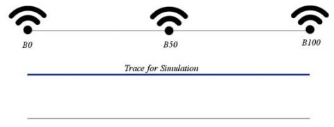
In our process, we first consider a straight 100m tunnel section with radio beacons placed in the 50m interval. With the three beacons present in our section, one at beginning ‘B0’ one at middle ‘B50’ 50m apart from ‘B0’ and last one at another end ‘B100’ as shown in Figure #!. Next, in our simulation of wireless positioning operation, we generate simulated RSSI readings along the trace of a moving tracker in this tunnel environment, considering the beacons are emitting radio waves that are propagating through tunnel roadway. How the radio wave propagates through the particular environment, which will decide the RSSI values at different points in the region. The simulation of this process has three main components.
1. The trace of target: In this study trace is a straight line moving at constant velocity.
2. Model errors in RSSI observation by the tracker.
3. Radio Propagation model through the tunnel.
The radio propagation behaviour in the tunnel-like environment has been studied and reported in the literature [18–21]. Next there are several distributions for modelling the wave path loss; namely, Rayleigh, Nakagami, Rice, Weibull and log-normal shadowing are among the most commonly used models.
Figure 2. Layout showing beacon positions in the 100m long tunnel section that is considered for simulation
For our simulation purpose, we choose Ray-Tracing model considering one reflection for propagation modelling; and for path loss to used log-distance path loss model. Compared to other models we prefered Ray-Tracing model for its mathematical simplicity [18] and ease of implementation fir the simulated cases. Coefficient used in the radio propagation model were derived from experimental readings, for reproduction of this work in some real mine or underground tunnel, an experimentally developed RSSI map can be used.
Figure 3. Simulated RSSI map of three beacons in the 100m gallery section
For the measurement likelihood model of the particle filter, this simulated RSSI map of the tunnel is used for the respective beacons in the simulation. And our ‘particle filter’ estimates observation vector of RSSI values for each particle using the values from this interpolated map generated using simulated observation points added with Gaussian noise with variance 5 units (of RSSI value) as sensor error.
3.1 Modeling the filter
The state estimation is the procedure of gaining information about the unknown state of a system by observing the other related quantity whose relationship with the state is mathematically modelled to sufficient extent. In a Bayesian framework, the state, as well as the measurement, are treated as stochastic vectors. The likelihood of measurement Z for given the state X be denoted by $\mathrm{P}\left(Z_{t} | X_{t}\right)$ where the subscript ‘t’ denotes the time instance in the particular stochastic process.
Localization problems, in general, is modelled as Hidden Markov Model (HMM), when developing ‘particle filter’ model or similar MCL based localization filters. The position state that we are trying to estimate is a hidden parameter as we are not able to measure it directly, but we have some sensor measurements and some prior knowledge and mathematical understanding of how the system behaves.
Figure 4. Abstract representation of tracking as HMM. $X_{t}$ refers to position state that is unknown and to be estimated and $Z_{t}$ refers to the sensor observation information
In case of radio beacon based positioning systems, the position of the tracker is the hidden variable. And the vivid heterogeneous sensor information such as RSSI readings observed by the tracker and the several other possibly useful information for indoor tracking is the observation or measurements vector that is represented as $Z_{t}$ in this paper.
Next, by considering the prior knowledge about the state X that is denoted by $\left(\overline{X_{t}}\right)$, a estimation and probability distribution of X we can get before obtaining the measurement, which is denoted by belief $\left(\overline{X_{t}}\right)$ where
belief (($\overline{X_{t}}$)=P($\overline{X_{t}}$|all the priory information) (1)
With this, we can formulate the joint density of the state and the observation we got from our sensors $\mathrm{P}\left(Z_{t},\left(\overline{X_{t}}\right)\right.$
P (($\overline{Z}_{t}$,( $\overline{X_{t}}$)=P ($Z_{t} | \overline{X_{t}}$)*belief ($\overline{X_{t}}$) (2)
With application of Bayesian theory, we can say
belief($X_{t}$) or P($X_{t} | Z_{t}$)= $\frac{\left(\mathrm{P}\left(Z_{t} | \overline{X_{t}}\right) * \text {belief}\left(\overline{X_{t}}\right)\right.}{P\left(Z_{t}\right)}$ (3)
In the formulation P($Z_{t}$) is incorporated in the normalization constant ‘η’ this is why there is no need for separate estimation. Finally the equation dealing with positioning takes the following form where prediction update computes the priori probability distribution belief($\overline{X_{t}}$) and the priory estimate then further corrected with the help of observations. The particle filtering is one of such technique which in general can be used to solve formulations such as this.
Predicted State
belief(($X_{t}$) )=∫{ P($X_{t} | X_{t-1}$), $U_{t}$)*belief($X_{t-1}$b)} d($X_{t-1}$) (4)
Correction after observation
belief($X_{t}$)=η*∫{ P($Z_{t} | \overline{X_{t}}$)*belief($\overline{X_{t}}$)} d($\overline{X_{t}}$) (5)
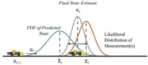
Figure 5. Illustration attempting to explain the mathematics behind the probabilistic tracking algorithm
The diagram above is very much simplified illustration of this mathematical formulation, however, in practice, these probability distributions are unknown and estimation of those probability distributions as to be done, by case specific models, developed using analytical derivation and experimental data.
$\mathrm{P}\left(X_{t} | X_{t-1}, U_{t}\right)$ this PDF in eq. 4 is related the state transition function of a particle filter, that helps to evolve the particles to the next state from a preceding state. It is used during the prediction step of the ‘particle filter’ Workflow in Figure 6. In our formulation, the state transition function assumes a Gaussian motion model with a constant velocity equal to the velocity given in the simulated trace of the tracker. The function uses a Gaussian distribution to determine the position of the particles in the next time step. In case of real application this has to be replaced with a suitable distribution that better represents the dynamics of the subject that is been tracked (e.g. pedestrians, drone, wheeled robot, mine car etc.)
Next, the trace of the tracker in our simulation is a straight line moving with a constant velocity thus in the posterior state in the motion model of the ‘particle filter’ we use the eq. 6
$X_{t+1}=X_{t}+\mathrm{V} * \delta \mathrm{t}+\sim \mathrm{N}\left(0, \Sigma_{p}\right)$ (6)
where, $\Sigma_{p}$ is the process noise covariance. And V is the velocity of tracker.
After predicting the next state, you can use measurements from sensors to correct your predicted state. This measurement likelihood function, by definition, gives a weight for the state hypotheses (each particle is a state hypothesis) based on a given measurement. The high value of likelihood represents a certainty that observed measurement actually matches with the RSSI values that the tracker has observed. This likelihood value is used as a weight for the state hypothesis represented by these particles. Although the prediction step can prove accurate for a small number of intermediate steps, however, to get accurate tracking, we use the sensor RSSI observations to correct the states of particles, by means of resampling.
Observation model in our case is derived from the simulated RSSI map of the beacons as shown in Figure 3. For any particle placed in the tunnel, we can get respective RSSI values for each beacon from the RSSI map that is shown in Figure 3. For our study the observation $\hat{Z}_{t}$=Vector of RSSI values measured for state $Z_{t}$.
Likelihood weight function in case of the real sensor observation vector is $Z_{t}$ taking it as multivariate normal.
Likelyhood= $\frac{\exp \left(-\frac{1}{2}\left(Z_{t}-\hat{Z}_{t}\right) \mathrm{T} \Sigma_{L}^{-1}\left(Z_{t}-\hat{Z}_{t}\right)\right)}{\sqrt{(2 \pi)^{k}\left|\Sigma_{L}\right|}}$ (7)
where, $\Sigma_{L}$=Likelihood covariance; k=number of beacons or the number of variable in the vector.
Figure 6. Workflow of the‘particle filter’ algorithm in this work
The radio propagation characteristic for underground tunnel environments is often more complicated than simplified ray tracing model, which don’t consider factors like wall roughness, interference etc. Still, for our study, this shall work fine as the motive of this study is to primarily study the performance of ‘particle filter’ and effect of different beacon deployment schemes in tunnel-like environment. That is why even the simplified radio propagation model like Ray tracing model with single reflection consideration shall server our purpose.
There is another important parameter that is the number of particles, each particle in the ‘particle filter’ is a state hypothesis that is tested against the observation model and the sensor data. Either the particle with the highest likelihood or the likelihood-weighted mean of all particles is taken to determine the best state estimate. In our application, we compute the best estimate by means of taking the likelihood-weighted average of all the particles. Finally for resampling the standard resampling policy described in [4] is used.
3.2 Design of experiment
As discussed before in section 2, we wish to observe the error in the estimation of ‘particle filter’ along with variance of error for same simulated data, with different ‘particle filter’ configuration. In our design of experiment (DOE) the process is the application of particle filter, the fixed input is the data from the simulation, and control parameters are the ‘particle filter’ configuration and beacon layout.
Fixed parameters in DOE
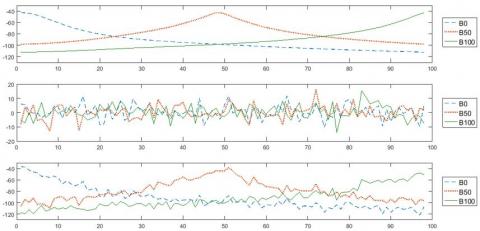
Form simulation we get time series data of RSSI readings measured by the tracker moving along the trace line (as shown in Figure 2). The data is generated with the help of simulated RSSI map (Figure 3) with the added Gaussian noise of variance 5 (unit of RSSI). Figure 7 shows the noisy RSSI data from each respective beacon which is used as input to the filter model. This input is kept as a fixed parameter in the experiment throughout.
Figure 7. Simulated time series data, above is noise free RSSI data; then additional Gaussian noise (middle); below is the noisy RSSI data from respective beacon which is used as input to the filter model
Control parameters
1 The first control parameter is beacon layout, where at the first case; we apply the ‘particle filter’ on considering the data only from ‘B0’ and ‘B100’ (2 beacons). And in another case, we consider data from all three beacons for position estimation.
2 Second control parameter that we vary is system noise covariance. The values of system noise covariance that were used in the experiment: 0.5 I, 1 I, 2 I, 5 I, 10 I, 20 I (‘I’ stands for identity metrics)
3 The third control parameter is Measurement Likelihood covariance, values used were: 1 I, 5 I, 10 I, 20 I, 50 I.
4 Fourth control parameter in the experiment was the number of the particle (state hypothesis) used while applying the filter on simulated data. The values taken for this control parameter were: 10, 20, 50, 100, 150, and 200.
Observations
We repeated the filtering process for 30 times for each combination of control parameters. And then we observed its whisker plots for analysis and interpretation of the results. The quantitative parameters that we observed and compared among the results were mainly the mean error in the estimated traces along the tunnel axis direction. And variance in that estimation for these 30 repeated applications of filters.
Few of the important results that we identified from the results we observed are discussed in this section.
4.1 Varying the number of particles
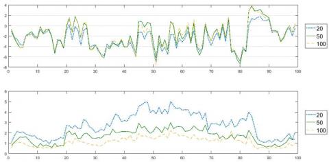
By varying the number of particles, we could see that accuracy improves with an increase in the particle. And more importantly, the variance of estimation for the 30 repetition decrease with increase in particle number.
Figure 8. Comparison of error (above) and variance (below) of ‘particle filter’ estimation with different number of particles
4.2 Varying the process noise
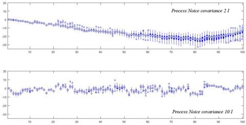
This is a qualitative observation that we make is with a low value of process noise there is a tendency of error accumulation. And at higher process noise ‘particle filter’ performs better in terms of accuracy.
Figure 9. Whisker plot of error from 30 repeated filter application for different process noise. With 100 particles, 20 I likelihood covariance and 2 beacon setup
4.3 Varying likelihood covariance
Figure 10. Comparison of ‘particle filter’ performance with different likelihood covariance. With 100 particles, 10 I process noise covariance and 2 beacon setup
4.4 With three beacons at 50m interval
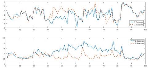
Improvement in position estimate with 3 beacon setup is marginal. However, we can find that standard deviation of estimation significantly reduces for 3 beacon setup, for estimated positions around the additional beacon ‘B50’ around the centre of the tunnel section.
Figure 11. Comparison of ‘particle filter’ performance with the addition of 'B50' beacon at the center of the tunnel. With 100 particles, 10 I process noise covariance and 20 I likelihood covariance
5.1 Insights on number of particles
From the results, we can understand the obvious fact that the number of particles we use in the filter place a vital role in the estimation. A low number of particles means incapability of capturing the states of possible estimates in a less dense manner, thus the best estimate is often missed out. As we can see in Figure 8 that reducing the number of particles reduces the estimation accuracies and increases the standard deviation. However, sometimes when state estimation has to be done on low powered embedded computers, in such situation we need to implement ‘particle filter’ with less number of particles. Though results may be poor, however, for cases where lack of precision is tolerable, there a particle filter with less number of particle too may work. This is why it was important to study the behaviour of the ‘particle filter’ with the particles as low as 50 and less. With our study, we get some idea that to what extent reduction in the number of particles influences the positioning estimate.
5.2 Insights on process noise covariance
Next, with the result, we also understand that for successful implementation of positioning with ‘particle filter’ we have to have a perfect balance between system noise or the process noise, and the covariance of likelihood function in the observation model. We can see in Figure 9 that if we keep system noise low, then there is a possibility that result from ‘particle filter’ may fail to give a right estimate. Figure 9 also shows that there is a higher tendency of error propagation in subsequent estimation by the filter in case of low process noise covariance. This propagation of error has potential to cause ‘particle filter’ to fail and diverge like of example in Figure 12. In such case, re-initialization of particle states can be one of the possible solutions to recover. At this study, no such approach was implemented in out ‘particle filter’ model that is used, as our intention at this point is to investigate the behaviour of the ‘particle filter’ and identify possible cases where ‘particle filter’ may fail. And Improving upon those limitations is in the future scope of this work.
Figure 12. A result showing the failure of ‘particle filter’ due to the accumulation of error due to low process noise covariance. With 100 particles, process noise 0.5 I, likelihood covariance 20 I and 2 beacons setup
5.3 Insights on of likelihood covariance
In the results shown in Figure 10, we can see that keeping the likelihood covariance in ‘particle filter’ model high leads to better accuracy. However, it also increases the variability of estimation as we could see in below plot of Figure 10. Previous studies on the behaviour of particles filter [2] also pointed out the importance of selecting a proper covariance matrix for process noise and likelihood covariance. Our results and analysis add additional in-depth insight and visual illustration of effects of different values of this covariance matrices. As discussed in section 5.2 that giving an increased process noise in the ‘particle filter’ model ensures better accuracy similarly giving increased covariance in the likelihood function helps increase the accuracy of estimation.
5.4 Insights on accuracy improvement with additional beacons
As we see in Figure 11 the comparison of error plots when the additional ‘B50’ beacon is considered. Addition of another beacon in the middle of the two existing beacon helped improving estimation by the filter. However, this improvement is marginal (when compared to two beacon setup). Yet another phenomenon we could see is that around the additional beacon ‘B50’ the mean error has reduced, and the variance has notably decreased around ‘B50’. The reason behind this phenomenon can be better appreciated if we see the simulated RSSI heat map of Figure 3 in a different representation of Figure 13. Where we can visually understand (seeing the gradient discontinuities) that around the beacons, change in RSSI value is more prominent with small changes in position, this is why small changes in tracker position were captured well when the simulated tracker was close to the beacon. Whereas when the tracker is away from the beacon, the RSSI value shows less spatial variation. This is how the addition of ‘B50’ beacon helped improve accuracy around the centre region of the tunnel as we could see in Figure 11.
Figure 13. Gradient map of radio beacon RSSI
From this study, we gather insights on how configuration parameters of particle filters influence the estimation accuracies. And our results also confirmed that deploying additional beacons have a contribution to the improvement in accuracy, and contribution of the additional beacon is more prominent in the vicinity of the area where the beacon is added.
From our analysis so far with fixed trace and a simplified prediction model we got some insight on the underlying mathematics of particle filter. Now our next step is to investigate further how ‘particle filter’ may work on tracking more complex subjects such as mobile ground vehicles, UAVs, Pedestrians etcetera in a tunnel-like environment; where the state prediction model has more complexity and uncertainties. Such studies have significance in pedestrian tracking and UAV localization in a tunnel-like environment of underground mine roadways, similar to the study [22]. Now it is also a matter of interest that how ‘particle filter’ handle those noises for these different types of target objects with different movement kinematics. With such analysis, we shall be able to make more meaningful conclusions.
[1] Gordon NJ, Salmond DJ, Smith AFM. (1993). Novel approach to nonlinear/non-Gaussian Bayesian state estimation. IEE Proceedings F - Radar and Signal Processing 140(2): 107–113. https://doi.org/10.1049/ip-f-2.1993.0015
[2] Gustafsson F. (2010). Particle filter theory and practice with positioning applications. IEEE Aerospace and Electronic Systems Magazine 25(7): 53–82. https://doi.org/10.1109/MAES.2010.5546308
[3] Hu XL, Schon TB, Ljung L. (2008). A basic convergence result for particle filtering. IEEE Transactions on Signal Processing 56(4): 1337–1348. https://doi.org/10.1109/TSP.2007.911295
[4] Arulampalam MS, Maskell S, Gordon N, Clapp T. (2002). A tutorial on particle filters for online nonlinear/non-Gaussian Bayesian tracking. IEEE Transactions on Signal Processing 50(2): 174–188. https://doi.org/10.1109/78.978374
[5] Gustafsson F, Gunnarsson F, Bergman N, Forssell U, Jansson J, Karlsson R, Nordlund PJ. (2002). Particle filters for positioning, navigation, and tracking. IEEE Transactions on Signal Processing 50(2): 425–437. https://doi.org/10.1109/78.978396
[6] Chirdon D, Barkand T, Damiano N, Dransite G, Hill J, Engineer M, Retzer P, Shumaker W. (2006). Emergency Communication and Tracking Committee Underground Communication and Tracking Systems Tests at CONSOL Energy Inc., McElroy Mine, MISHA
[7] Griffin KR, Schafrik SJ, Karmis M. (2010). Designing and modeling wireless mesh communications in underground coal mines. 2010 SME Annual Meeting, SME, Phonex, AZ, 10–066
[8] Schafrik SJ. (2013). Underground Wireless Mesh Communication Infrastructure Design Prediction and Optimization (Doctoral)Virginia Polytechnic Institute and State University Retrieved from https://vtechworks.lib.vt.edu/handle/10919/19365
[9] Yu J. (2015). A Layered Two-Step Hidden Markov Model Positioning Method for Underground Mine Environment Based on Wi-Fi Signals. Masters Thesis, Mid Sweden University
[10] Hawkins W, Daku BLF, Prugger AF. (2005). Vehicle localization in underground mines using a particle filter, Electrical and Computer Engineering, 2005. Canadian Conference On, IEEE 2159–2162
[11] Hawkins W, Daku BLF, Prugger AF. (2006). Positioning in Underground Mines. IECON 2006 - 32nd Annual Conference on IEEE Industrial Electronics. 3139–3143. https://doi.org/10.1109/IECON.2006.347889
[12] Errington AFC, Daku BLF, Prugger AF. (2007). Vehicle Positioning in Underground Mines, 2007 Canadian Conference on Electrical and Computer Engineering. https://doi.org/10.1109/CCECE.2007.151
[13] Song B, Zhang S, Long J, Hu Q. (2017). Fingerprinting localization method based on toa and particle filtering for mines, Mathematical Problems in Engineering.
[14] Thrun S, Fox D, Burgard W, Dellaert F. (2001). Robust Monte Carlo localization for mobile robots, Artificial Intelligence 128(1): 99–141. https://doi.org/10.1016/S0004-3702(01)00069-8
[15] Wu Z, Jedari E, Muscedere R, Rashidzadeh R. (2016). Improved particle filter based on WLAN RSSI fingerprinting and smart sensors for indoor localization. Computer Communications 83: 64–71. https://doi.org/10.1016/j.comcom.2016.03.001
[16] Pak JM, Ahn CK, Shmaliy YS, Lim MT. (2015). Improving Reliability of Particle Filter-Based Localization in Wireless Sensor Networks via Hybrid Particle/FIR Filtering. IEEE Transactions on Industrial Informatics 11(5): 1089–1098. https://doi.org/10.1109/TII.2015.2462771
[17] Pak JM, Ahn CK, Shi P, Shmaliy YS, Lim MT. (2017). Distributed hybrid particle/FIR filtering for mitigating nlos effects in TOA-based localization using wireless sensor networks. IEEE Transactions on Industrial Electronics 64(6): 5182–5191. https://doi.org/10.1109/TIE.2016.2608897
[18] Forooshani AE, Bashir S, Michelson DG, Noghanian S. (2013). A Survey of Wireless Communications and Propagation Modeling in Underground Mines. IEEE Communications Surveys Tutorials 15(4): 1524–1545. https://doi.org/10.1109/SURV.2013.031413.00130
[19] Bedford MD, Kennedy GA, Foster PJ. (2017). Radio transmission characteristics in tunnel environments. Mining Technology 126(2): 77–87. https://doi.org/10.1080/14749009.2016.1259196
[20] Zhou C, Plass T, Jacksha R, Waynert JA. (2015). RF Propagation in Mines and Tunnels: Extensive measurements for vertically, horizontally, and cross-polarized signals in mines and tunnels. IEEE Antennas and Propagation Magazine 57(4): 88–102. https://doi.org/10.1109/MAP.2015.2453881
[21] Patri A, Nimaje DS. (2015). Radio frequency propagation model and fading of wireless signal at 2.4 GHz in an underground coal mine. Journal of the Southern African Institute of Mining and Metallurgy 115(7): 629–636. https://doi.org/10.17159/2411-9717/2015/V115N7A9
[22] Özaslan T, Shen S, Mulgaonkar Y, Michael N, Kumar V. (2015). Inspection of Penstocks and Featureless Tunnel-like Environments Using Micro UAVs, L. Mejias; P. Corke; J. Roberts (Eds.), Field and Service Robotics, Springer International Publishing, Cham 105: 123–136. https://doi.org/10.1007/978-3-319-07488-7_9