Fixed ground-target tracking control of satellites using a nonlinear model predictive control

In the approach of MPC, or alternatively receding horizon control, the optimal solution of the control problem, called the control input is found by solving a constraint optimization problem at each time instant with a moving horizon. This results in a control law with a feedback nature. Actually, optimization problem of the constraint objective function can be converted into a root finding problem of a set of nonlinear equations. These nonlinear equations are obtained by means of applying necessary conditions for optimality [1]. 

A general nonlinear dynamic system can be represented as:

$\begin{aligned} \dot{x}(t)=& f(x(t), u(t), p(t)) \\ & x\left(t_{0}\right)=x_{o} \end{aligned} \}$ (1)

where, $x(t) \in R^{n}$ is a state vector with states, $u(t) \in R^{m_{u}}$ is an input vector with mu inputs and $p(t) \in R^{m_{p}}$ is a time-varying vector. The optimal control problem for this system where a cost function is minimized while satisfying ng-dimensional equality constraints g and ng-dimensional inequality constraints h are represented as [1]:

$\begin{aligned} \underset{u}{\operatorname{minimize}} : J=\varphi &\left(x\left(t_{f}\right), p\left(t_{f}\right)\right) \\ &+\int_{t_{0}}^{t_{f}} L(x(\dot{t}), u(\dot{t}), p(\dot{t})) d \dot{t} \end{aligned}$

subjected.to $\left\{\begin{aligned} \dot{x}(t)=& f(x(t), u(t), p(t)) \\ & x\left(t_{0}\right)=x_{o} \\ g(x(t), u(t), p(t)) &=0 \\ h(x(t), u(t), p(t)) & \leq 0 \end{aligned}\right.$ (2)

where, $T=t_{f}-t_{0}$ is the prediction horizon,  $\varphi( .)$ represents the terminal cost at the end of the prediction horizon and $L( .)$ denotes the trajectory cost over the horizon. The actual state x(t) is used as the initial state for the optimal control problem over the horizon $[t, t+T]$ .

Although the control input is determined over this horizon, the actual submitted input as a feedback to the system is the only optimum value at the initial time of this current horizon [1,4,5].

Solving an optimization problem with inequality constraints is not an easy task because of the complexity of the optimality conditions known as Karush–Kuhn–Tucker (KKT) conditions.  In this case, a particular interior point method known as barrier method is used to convert the inequality constraints to equality constraints. So, if $h_{i} \leq 0$ it can be written as $h_{i}+\alpha_{i}^{2}=0$ where $\alpha_{i}$ is a dummy input. If the problem is feasible, in the end, $h_{i}=-\alpha_{i}^{2}$ and for any given real value for $\alpha_{i}$, $h_{i} \leq 0$ The integrant part in cost function presented in Equation (2) has been also modified by adding a term $-r^{T}$ that is to give incentive to the solver to stay away from the boundaries of the feasible set [1,4].  Thus, the optimal control problem can be modified as:

$\begin{aligned} & \underset{u, \alpha}{\operatorname{minimize}} \cdot J=\varphi\left(x\left(t_{f}\right), p\left(t_{f}\right)\right) \\+& \int_{t_{0}}^{t_{f}}\left(L(x(\dot{t}), u(\dot{t}), p(\dot{t}))-r^{T} \alpha(\dot{t})\right) d \dot{t} \end{aligned}$

subjected.to $\left\{\begin{aligned} \dot{x}(t)=& f(x(t), u(t), p(t)) \\ & x\left(t_{0}\right)=x_{o} \\ g(x(t), u(t), p(t)) &=0 \\ h(x(t), u(t), p(t))+\alpha(t)^{2} &=0 \end{aligned}\right.$ (3)

So, if the entries of are small positive numbers, the solution of this modified optimization problem is close to the solution of the original one with inequality constraints. Expanding the input vector u(t) to contain not only the real inputs but also the dummy inputs and considering  is the final equality constraints with dimension $m_{c}=m_{h} \cdot+m_{g}$ including the original equality constraints and the converted inequality constraints to equality constraints, the optimal problem can be written in more useful and generalized form as following [1,4]:

$\begin{aligned} \underset{u}{\operatorname{minimize} : J}=\varphi &(x(t+T), p(t+T)) \\ &+\int_{t}^{t+T} L(x(\dot{t}), u(\dot{t}), p(\dot{t})) d \dot{t} \end{aligned}$

Subjected to: $\left\{\begin{array}{c}{\dot{x}=f(x(t), u(t), p(t))} \\ {x(t)=x_{o}} \\ {C(x(t), u(t), p(t))=0}\end{array}\right.$ (4)

where, the optimal control $u^{*}(\dot{t} ; t, x(t))$ that minimize J is calculated over $\dot{t} \in[t, t+T]$, and its initial value at initial time t, $u^{*}(t ; t, x(t))$ is used as actual control input u(t) to the system.  The functions $\varphi$ and L

$\varphi=\frac{1}{2}\left(x(t+T)-x_{f}\right)^{T} S_{f}\left(x(t+T)-x_{f}\right)$ (5)

$L=\frac{1}{2}\left(\left(x-x_{f}\right)^{T} Q\left(x-x_{f}\right)+u^{T} R \cdot u-r^{T} \alpha\right) )$ (6)

where S_f, Q, and R are free parameters' weighting matrices.

The NMPC problem is basically a family of finite horizon optimal control problems (FHOCPs) along fictitious time $\tau$ as follows [1,4]:

$\begin{aligned} \text { Minimize } & : J=\varphi\left(x^{*}(T, t), p(t+T)\right) \\ &+\int_{0}^{T} L\left(x^{*}(\tau, t), u^{*}(\tau, t), p(t+\tau)\right) d \tau \end{aligned}$

Subjected.to $\left\{\begin{array}{c}{x_{\tau}^{*}(\tau, t)=f\left(x^{*}(\tau, t), u^{*}(\tau, t), p(t+\tau)\right)} \\ {x^{*}(0, t)=x(t)} \\ {C\left(x^{*}(\tau, t), u^{*}(\tau, t), p(t+\tau)\right)=0 \cdots}\end{array}\right.$ (7)

where subscript $\tau$ represents partial differentiation with respect to $\tau$. The new state vector, $x^{*}(\tau, t)$, denotes a trajectory along the $\tau$ axis starting from $x(t) \cdot \operatorname{at} \tau=\cdot 0$. The optimal control input, $u^{*}(\tau, t)$, is obtained on the $\tau$ axis as the solution to FHOCP for each t, and actual control input is set by $u(t)=u^{*}(0, t)$. Horizon T is commonly a function of time, $T=T(t)$ .

To solve an optimization problem subject to equality constraints Lagrange multipliers method is used. The way it works is to write the Hamiltonian function as a sum of the integrant part of the cost function plus the dynamic equations multiplied by Lagrange multiplier $\lambda^{\prime} s$  known as costates plus the constraints equations multiplied by Lagrange multiplier $\boldsymbol{\mu}^{\prime} \boldsymbol{s}$ as seen in the following equation [1].

$\mathcal{H}(x, \lambda, u, \mu, p)=L(x, u, p)+\lambda^{T} f(x, u, p)+\mu^{T} C(x, u, p)$ (8)

Once the Hamiltonian function is defined, the first-order conditions necessary for optimal control is getting by calculus of variation as Euler Lagrange Equations (ELEs) [4].

$x_{\tau}^{*}=f\left(x^{*}, u^{*}, p\right)$ (9)

$x^{*}(0, t)=x(t)$ (10)

$\lambda_{\tau}^{*}=-\mathcal{H}_{x}^{T}\left(x^{*}, \lambda^{*}, u^{*}, \mu^{*}, p\right)$ (11)

$\lambda^{*}(T, t)=\varphi_{x}^{T}\left(x^{*}(T, t), p(t+T)\right)$ (12)

$\mathcal{H}_{u}\left(x^{*}, \lambda^{*}, u^{*}, \mu^{*}, p\right)=0$ (13)

$C\left(x^{*}, u^{*}, p\right)=0$ (14)

where the argument of p  is $t+\tau$ when absent. The ELEs describe a TPBVP, in which the value of initial state is known whereas the terminal costate is a function of the terminal state. Nonlinear TPBVP has to be solved within the sampling period for measured state x(t) at each sampling time, which represents a hard-computational load and is one of the major problems in NMPC. Now with discretizing these conditions for optimality on $\tau$-axis with forward difference by dividing the horizon into N time steps as follows [4].

$x_{i+1}^{*}(t)=x_{i}^{*}(t)+f\left(x_{i}^{*}(t), u_{i}^{*}(t), p(t+i \Delta \tau)\right) \Delta \tau$ (15)

$x_{0}^{*}(t)=x(t)$ (16)

$\lambda_{i}^{*}=\lambda_{i+1}^{*}+\mathcal{H}_{x}^{T}\left(x_{i}^{*}(t), \lambda_{i+1}^{*}(t), u_{i}^{*}(t), \mu_{i}^{*}(t), p(t+i \Delta \tau)\right) \Delta \tau$ (17)

$\lambda_{N}^{*}(t)=\varphi_{x}^{T}\left(x_{N}^{*}(t), p(t+T)\right)$ (18)

$\mathcal{H}_{u}^{T}\left(x_{i}^{*}(t), \lambda_{i+1}^{*}(t), u_{i}^{*}(t), \mu_{i}^{*}(t), p(t+i \Delta \tau)\right)=0$ (19)

$C\left(x_{i}^{*}(t), u_{i}^{*}(t), p(t+i \Delta \tau)\right)=0$ (20)

where time step $\Delta \tau=T / N$ and the real-time t is kept continuous while fictitious time $\mathrm{E} \tau$ is discretized. The computed sequences of the state, costate, input, and Lagrange multiplier on the discretized horizon are represented by $\left\{x_{i}^{*}(t)\right\}_{i=0}^{N}, \quad\left\{\lambda_{i}^{*}(t)\right\}_{i=0}^{N} \quad, \quad\left\{u_{i}^{*}(t)\right\}_{i=0}^{N} \quad$ and $\quad\left\{\mu_{i}^{*}(t)\right\}_{i=0}^{N}$, respectively.

Consequently, NMPC is formulated as TPBVP in Equation (15-20) for measured state x(t)  at real time t. The Equations (15,16) are the system dynamic equations with its initial conditions. The next two Equations (17,18) are dynamic equations corresponding to the Lagrange multiplier costates $\lambda$ with its final conditions. The rest of equations are equality constraints on all the variables that include the partial derivative of the Hamiltonian with respect to vector u, the vector of real and dummy inputs, and also the derivative of the Hamiltonian with respect to vector $\mu$ which lead to total equality constraints equation C=0 .

MPC is to solve an optimal control problem in each time step of a discrete time controller.  While the system is working the current states xn are measured or estimated then the optimal control problem is solved by computing the input ui for the next N steps and only the first step of the sequence is returned and that is the computed input which should be applied to the system then this loop is repeated again and again. Therefore, MPC is an implementation of an optimal controller in a real time.

In fact, the efficient control performance of the NMPC scheme is always obstructed by the limited model precision. As for the complicated satellite dynamics with time-varying parameters and nonlinear characteristics, the used model may have some errors in addition to unexpected disturbance. Moreover, for the optimal tracking problem, the error dynamic model is crucial for the robust control design. Therefore, a new control-oriented model based on the attitude and rate errors is designed in this paper. Doing that allows handling the tracking task as a simple regulation task.

In this section, the main tracking problem is converted into a well-formulated global and simple regulation problem. The simple regulation problem is a more traceable problem and has a great potential dealing with disturbance and uncertainty. The attitude kinematic equation using quaternion error representation is described in [7] considering the inertial frame as a reference frame. The satellite is assumed to start GTT task from nadir pointing attitude and hence the orbital frame is used as a reference frame instead of the inertial frame for simplicity purposes. Thus, the attitude kinematic equation using quaternion error representation can be reformulated as:

$\delta \dot{\overline{q}}=0.5 \Omega(\delta \omega) \delta \overline{q}$ (35)

where

$\delta \omega=\omega_{S B C}^{O R C}-A_{d}^{S B C} \omega_{d}^{O R C}$ (36)

$\delta \overline{q}=\left[\begin{array}{c}{\boldsymbol{q}_{\boldsymbol{e}}} \\ {q_{4 e}}\end{array}\right]=\left[\begin{array}{cccc}{q_{4 d}} & {q_{3 d}} & {-q_{2 d}} & {-q_{1 d}} \\ {-q_{3 d}} & {q_{4 d}} & {q_{1 d}} & {-q_{2 d}} \\ {q_{2 d}} & {-q_{1 d}} & {q_{4 d}} & {-q_{3 d}} \\ {q_{1 d}} & {q_{2 d}} & {q_{3 d}} & {q_{4 d}}\end{array}\right]\left[\begin{array}{c}{q_{1}} \\ {q_{2}} \\ {q_{3}} \\ {q_{4}}\end{array}\right]$ (37)

The subscript d represents the desired frame, $\boldsymbol{\Omega}(\delta \omega)$ is 4*4 skew matrix function, the $\delta \overline{q}$  represents the quaternion error from the desired to the body frame, $\omega_{S B C}^{O R C}$ represents desired quaternion, q represents the current attitude, $\delta \omega$ is the error in angular rate represented in the body frame, $\omega_{S B C}^{O R C}$ is the orbital referenced body angular rate in body frame, $\omega_{d}^{O R C}$ is the orbital referenced desired angular rate in the desired frame and $A_{d}^{S B C}$ is the transformation matrix from desired to body frame.

The dynamic model of an Earth-pointing satellite using reaction wheels (RWs) only as active actuators is given by:

$J \dot{\omega}_{S B C}^{O R C}=N_{\omega o}+N_{G G}-\omega_{S B C}^{E I C} \times\left(J \omega_{S B C}^{E I C}+h_{w}\right)-\dot{h}_{w}$ (38)

Using Equation (36) to express the body angular rate $\omega_{S B C}^{O R C}$ as:

$\omega_{S B C}^{O R C}=\delta \omega+A_{d}^{S B C} \omega_{d}^{O R C}$ (39)

Differentiating Equation (39) to get

$\dot{\omega}_{B}^{O R C}=\delta \dot{\omega}-\Omega(\delta \omega) A_{d}^{S B C} \omega_{d}^{O R C}+A_{d}^{S B C} \dot{\omega}_{d}^{O R C}$ (40)

where $\Omega(\delta \omega)$ is $3 \times 3$ is skew matrix. Multiplying Equation (40) by J leads to

$J \dot{\omega}_{S B C}^{O R C}=J \delta \dot{\omega}-J\left[\Omega(\delta \omega) A_{d}^{S B C} \omega_{d}^{O R C}-A_{d}^{B} \dot{\omega}_{d}^{O R C}\right]$ (41)

Substituting $J \dot{\omega}_{B}^{O R C}$ from Equation (41) in Equation (38) gives:

$\begin{aligned} J \delta \dot{\omega}=& N_{\omega o}+N_{G G}+J &[ & \Omega(\delta \omega) A_{d}^{S B C} \omega_{d}^{O R C}-\\ & A_{d}^{S B C} \dot{\omega}_{d}^{O R C} ]-\omega_{S B C}^{E I C} \times\left(J \omega_{S B C}^{E I C}+h_{w}\right)-\dot{h}_{w} \end{aligned}$ (42)

Generally, the terms N_GG  and $N_{\omega O}$ and $\omega_{S B C}^{E I C} \times\left(J \omega_{S B C}^{E I C}+h_{w}\right)$, are not significant for many practical rotation maneuvers [8]. The term $\dot{\omega}_{d}^{O R C}$ can also be neglected as it is lower several orders of magnitude than other terms for nearly circular orbit. All the omitted terms can be considered as some types of uncertainty which can be handled effectively using such presented model. Robustness check in the simulation is also used to confirm the validity of NMPC with the presented model in general. Rewriting Equation (42) in more simple and efficient form after neglecting the smaller terms yields:

$J \delta \dot{\omega}=J \Omega(\delta \omega) A_{d}^{S B C} \omega_{d}^{O R C}+u_{w}$

$\dot{h}_{w}=-u_{w}$ (43)

where u_w  represents the RWs torque. Equation (35) and Equation (43) are the control-oriented model or in other words, the tracking error dynamic model used in this paper. This model has 10 states represented in attitude quaternion error, rate error, and RWs momentum. The model also includes time-varying parameter represented in $A_{d}^{S B C} \omega_{d}^{O R C}$ which add a little bit difficulty in implementation. The desired rate $\omega_{d}^{O R C}$ is [8]:

$\omega_{d}^{O R C}=u_{S / T}^{O R C} \times \dot{u}_{S / T}^{O R C}$ (44)

where $u_{S / T}^{O R C}$ is unit direction vector of the direction from satellite to the target represented in orbit frame, $X_{S / T}^{O R C}$ computed by [8]:

$X_{S / T}^{O R C}=A_{E I C}^{O R C}\left(A_{E F C}^{E I C} X_{T}^{E F C}-r_{s a t}\right)$ (45)

as $r_{s a t}$ is the satellite position in Earth-centered inertial frame, $X_{T}^{E F C}$ is the target location in Earth-centered fixed frame and the transformation matrix $A_{E F C}^{E I C}$ from the fixed frame to the inertial is time-dependent matrix can be estimated considering constant Earth angular rate around its rotation axis, $\omega_{E}$ in the tracking maneuver period and knowing the initial phase , $\alpha_{G}$ between the x-axes of both EFC and EIC frames at t=0 as:

$A_{E F C}^{E I C}=\left[\begin{array}{ccc}{\cos \left(\omega_{E} t+\alpha_{G}\right)} & {-\sin \left(\omega_{E} t+\alpha_{G}\right)} & {0} \\ {\sin \left(\omega_{E} t+\alpha_{G}\right)} & {\cos \left(\omega_{E} t+\alpha_{G}\right)} & {0} \\ {0} & {0} & {1}\end{array}\right]$ (46)

The transformation matrix $A_{E I C}^{O R C}$ from the inertial frame to orbital frame can be deduced by using the satellite position r_sat  and velocity v_sat  in the inertial frame as [8]:

$A_{E I C}^{O R C}=\left[\begin{array}{lll}{\hat{u}} & {\hat{v}} & {\widehat{w}}\end{array}\right]^{T}$ (47)

where the unit vectors $\widehat{u}$,  $\hat{v}$ and $\widehat{w}$ are:

$\begin{aligned} \widehat{w} &=-\frac{r_{s a t}}{\left\|r_{s a t}\right\|} \\ \hat{v}=&-\frac{r_{s a t} \times s a t}{\left\|r_{s a t} \times v_{s a t}\right\|} \\ \hat{u} &=\hat{v} \times \widehat{w} \end{aligned} \}$ (48)

The vector $\dot{u}_{S / T}^{O R C}$ can be calculated as following [8]:

$\dot{u}_{S / T}^{O R C}=\frac{1}{\left\|X_{S / T}^{O R C}\right\|}\left[I_{3}-u_{S / T}^{O R C}\left(u_{S / T}^{O R C}\right)^{T}\right] \dot{X}_{S / T}^{O R C}$ (49)

where the time derivative $\dot{X}_{S / T}^{O R C}$  is calculated by differentiating Equation (45) to get the following [8]:

$\dot{X}_{S / T}^{O R C}=\dot{A}_{E I C}^{O R C}\left(A_{E F C}^{E I C} X_{T}^{E F C}-r_{s a t}\right)+A_{E I C}^{O R C}\left(\dot{A}_{E F C}^{E I C} X_{T}^{E F C}-\right.$

$v_{s a t} )$ (50)

The time derivative of transformation matrices $A_{EIC}^{ORC}$ and $A_{\text{EFC}}^{\text{EIC}}$ in Equation (50) are calculated as following [8]:

$\dot{A}_{EIC}^{ORC}={{[\hat{\dot{u}}\text{ \hat{\dot{v}} \hat{\dot{w}}}]}^{T}}$ (51)

Where

$\left. \begin{matrix}   \hat{\dot{w}}=-\frac{1}{\left\| {{r}_{sat}} \right\|}({{I}_{3}}-\bar{w}{{{\bar{w}}}^{T}}){{v}_{sat}} \\\hat{\dot{v}}=0\\   \hat{\dot{u}}=\frac{1}{\left\| {{r}_{sat}} \right\|}\hat{v}\times [({{I}_{3}}-\bar{w}{{{\bar{w}}}^{T}}){{v}_{sat}}]  \\\end{matrix} \right\}$  (52)

\[\dot{A}_{EFC}^{EIC}={{\omega }_{E}}\left[ \begin{matrix}   -\sin ({{\omega }_{E}}t+{{\alpha }_{G}})-\cos ({{\omega }_{E}}t+{{\alpha }_{G}})\text{ 0}  \\   \cos ({{\omega }_{E}}t+{{\alpha }_{G}})-\sin ({{\omega }_{E}}t+{{\alpha }_{G}})\text{   0}  \\   0\text{  0   0}  \\\end{matrix} \right]\] (53)

The transformation matrix  A_d^SBC in Equation (43) can be extracted easily from the quaternion error $\delta \text{\bar{q}}$ given in Equation (37). The desired quaternion q_d can be estimated as following [8]:

${{q}_{d}}=\left[ \begin{matrix}{{u}_{c}}\sin \frac{\delta }{2} \\\cos \frac{\delta }{2}  \\\end{matrix} \right]$ (54)

where δ is the angle between the time-dependent vector $u_{S/T}^{ORC}$ and commissioned axis or payload axis represented in body frame $u_{com}^{\text{SB}C}$ while u_c define the axis of rotation needed for constructing q_d given by [8]:

${{u}_{c}}=\frac{u_{com}^{SBC}\times u_{S/T}^{ORC}}{\left\| u_{com}^{SBC}\times u_{S/T}^{ORC} \right\|}$ (55)

The tracking error can be examined by calculating θ_err  to define the angle between $u_{com}^{\text{SB}C}$ and $u_{S/T}^{ORC}$ vectors as [8]:

${{\theta }_{err}}={{\cos }^{-1}}(u_{S/T}^{SBC}\centerdot u_{S/T}^{ORC})$ (56)

where the unit vector $u_{S/T}^{\text{SB}C}$ defined for the current attitude matrix $A_{ORC}^{\text{SB}C}$ as:

$u_{S/T}^{SBC}=A_{ORC}^{SBC}\centerdot u_{S/T}^{ORC}$ (57)

In order to evaluate the performance of using algorithm C/GMRES in solving a ground target tracking problem, the configuration UoSAT-12 satellite with higher RWs capabilities is used in the simulation. The inertia matrix J of the satellite in kgm² is diag(40,40,32).

Table 1.  Controller and simulation parameters

Three reaction wheels installed in a three-axis configuration to allow full control of the satellite attitude orientation with maximum torque $\pm 0.2\text{Nm}$ and momentum capacity $\pm 6\text{Nmsec}$. The working orbit is almost circular with altitude 650km,  inclination angle 64.5deg, right ascension of ascending node 10deg, initial mean anomaly  0deg and initial mean phase 0deg. The tracked fixed ground-target in EFC frame is [4021.9  -35.1   4933.6]^T The satellite commissioned axis is [1  -1  9]^T and the satellite attitude is assumed initially aligned with orbit frame.

During simulation perfect attitude knowledge and measurements of the vectors r_sat  and v_sat are assumed. The developed code of C/GMRES method is outputted as an ANSI/C standard source code for simulation purposes in this paper. In Table  1 a list of all the controller variable and simulation parameters used during simulation for GTT task.

Since the clear desired states for reformulated regulation problem represented in the attitude quaternion and angular rate, it is planned to lightly punish the deviation between the desired zero angular momentum and realized momentum during optimum solution searching.

Actually, the restrict requirements concern the trajectory of angular momentum change is considered in the limits put on the input vector real elements (the first three elements in the input vector). All parameters which have no real physical limits are allowed to be changed freely that is why their corresponding weighting values are relatively too low.

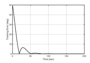
UoSAT -12 conveys two redundant 32m ground sampling distance (GSD) multi-spectral cameras to provide 64Km wide swath width [11]. Furthermore, UoSAT-12 also carries a high-resolution narrow-angle panchromatic camera with 10m GSD and 10Km swath [11]. The stability requirement during imaging to obtain acceptable image quality with relaxed maximum pixel smear in percentage 17% as explained in section (‎5) is computed and found to be better than  0.1 deg/sec.  It can be realized from Figure 1 and Figure 2 that the satellite needs only (≈ 200 sec) to be kept in a stable tracking mode with a very small tracking error defined in Equation (56), ${{\theta }_{err}}\approx 0.0045\deg $.

The supreme advantage here is that the proposed controller succeeded to maintain this precise tracking error during the overpass flight simulation time. Normally this accuracy is deteriorated whenever the satellite position becomes closer to the target. The resultant bell-shaped figure with maximum satellite angular slew rate at a closer position to the target violate the stability conditions needed for shooting with accepted image quality. The proposed tracking controller here can react as fast as the kinematic of the target. Keeping the tracking error within this precise limit during the overpass flight of the target allows shooting this target at any time. Hence, an additional shooting mode covering stereo triplets imaging and video surveillance can be carried out.

1.jpg

Figure 1. Tracking error

2.jpg

Figure 2. Tracking error zoom in

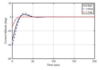
The Euler angles representing the satellite attitude change related to the desired frame is shown in Figure 3. The initial attitude mismatch is diminished fast.

3.jpg

Figure 3. Current attitude in Euler angles

The angular rate error of the satellite body is shown in Figure 4 during the tracking control. It is seen that the that the orbit-referenced angular velocity of the satellite body $\omega _{B}^{ORC}$ follows the desired angular rate command $\omega _{\text{d}}^{ORC}$ without a noticeable error during the tracking period.

The stability requirement (better than 0.1deg/sec) during imaging to obtain acceptable image quality is initially guaranteed after only 57sec as cleared from Figure 5. Fortunately, this stability guarantee is kept through over the target overpass flight simulation time.  From  Figure 2 and Figure 5,  the shooting conditions with minimum geo-location error is guaranteed after 200sec of starting tracking process with tracking error 0.0045 deg.

4.jpg

Figure 4. Satellite angular rate error

5.jpg

Figure 5. Current angular rate

The geo-location error due to this error will be 0.05km. Therefore, the high-resolution narrow-angle panchromatic camera which offers 10Km swath (i.e. image size 10*10) can be used efficiently while tracking with the proposed intelligent tracking controller. The steady-state quaternion error q_e=[0 0 0 1]^T  represented in Figure 6 means that body attitude is totally aligned with the desired attitude.

6.jpg

Figure 6. Quaternion error

Since the UoSAT-12 satellite is equipped with body-fixed imager, aligning the body attitude with the desired attitude means that this imager (payload) pointing at the target.

The activity of the three-axis RWs is shown in Figure 7  and Figure 8. Figure 7 confirms that the torques of the three-axis RWs are generally far from saturation limits (0.2Nm) during the duration needed for tracking the ground target. A wheel torque transient, in general, happens at the beginning of the tracking maneuver due to initial attitude error between the satellite payload axis and the desired target direction. The max torque provided by the RW of Y-axis and it is almost (0.19Nm) with very limited duration time. Once the controller starts to respond to the desired command, this attitude error starts to be reduced and hence the torques needed from RWs are decreased.

The angular momentums of the three-axis RWs in Figure 8 are far from angular momentum capacity h_wmax  (6.0Nm sec) during tracking task with the proposed controller. This safe working momentum region allows the RWs to further compensate for any disturbance easily and increase the robustness of the system as whole. It is also noticed that for this specific target and selected commissioned axis the effort needed from RW of Z-axis is minor however the other RWs provide the main effort for carrying out the required tracking maneuver. Since the disturbance is not considered during simulation, it is logic to note that the angular momentums of the RWs are kept unchangeable after achieving the tracking task.

7.jpg

Figure 7. Wheel torque

8.jpg

Figure 8. Wheel momenta

9.jpg

Figure 9. Robustness check against uncertainty in MOI

Because of the feedback nature of the proposed C/GMRES controller, the robustness of this controller against model uncertainties is guaranteed. Simulations were also done to examine the robust performance of the proposed tracking controller against a ±20% error in the moment of inertia of the satellite. These simulations demonstrate that the precise tracking error can still be preserved to designed values ± 0.003 degree as shown in Figure 9. However, in practice, the TE will ultimately be impacted by the attitude determination accuracy as well as the orbital measurements of the position and velocity vectors from the GPS receiver which have been not considered in this study.