OPEN ACCESS
China has become the world's largest trading goods nation in 2013, meanwhile, the trade value of import and export in Inner Mongolia was 11.99 billion U.S. dollars, which is the highest one over the years, however, the border trade value which accounts for nearly a third of the whole trade increased by years but never comes to the highest value. Based on the relevant data of Inner Mongolia border trade and industrial structure, the long-term effects of border trade on industrial structure will be testified in this thesis.
Inner Mongolia border trade, Industrial structure, Effect
The thesis focuses on analyzing the effect of regional industrial structure on the development of the border trade in certain region. Bases on the VAR model building on the correlated variables, adopting the relevant data of Inner Mongolia border trade and industrial structure, the long-term and short-term effects of border trade on industrial structure will be testified by the empirical test in this thesis.
2.1. Variable selection of empirical test
(1) The selection and measurement of the dependent variable.
Structure on foreign trade in certain region or country, industrial structure refers to the alteration of the industrial, including the speed and the direction. When establishing the index system of industrial structure alteration in early stages, the scholars placed particular emphasis on the speed of the industrial structure alteration; however, later some scholars realized that the speed of the industrial structure alteration couldn’t reflect the overall alteration of the industrial structure. Given this, some scholars proposed that the certain industrial value as the share of GDP should be used to measure the industrial structure alteration, which could embody the speed and the direction at the same time. The formula is:
${{y}_{1}}=\frac{outpu{{t}_{i}}}{GDP}$ (1)
Output is the added value of i industry. Due to the fact that China, especially the Inner Mongolia is in the development phase of industrialization, the thesis uses the added value of the secondary industry as the share of GDP to measure yl. Moreover, according to the law of Petty- Clark, at present, the direction of the industrial structure alteration in Inner Mongolia should follow such law, that is, the ratio of the primary and the tertiary industry will decrease, and the ratio of the secondary industry will increase; or the ratio of the primary and the secondary industry will decrease, and the ratio of the tertiary industry will increase. The first mention of the two illustrates that the industrial development is the primary one in Inner Mongolia; the latter illustrates that Inner Mongolia has stepped onto service economy age.
In addition, this thesis also adopts the index of the industrial structure alteration raised by Lan Qingxin and Tian Haifeng to measure the alteration of the industrial structure in Inner Mongolia. In this way, whether the foreign trade can cause the alteration of industrial structure can be improved, meanwhile, the reliability of the test can be improved too. The construction method of the index of the industrial structure alteration raised by Lan Qingxin and Tian Haifeng is like this:
Assume that economic aggregate(Y) is made up of n index, the formula should be:
$Y=\sum\limits_{i}^{n}{{{Y}_{i}}}$ (2)
Yi refers to the components of economic aggregate, then define the value i=1, 2, n. the following formula can be got.
${}^{dY}/{}_{Y}=\sum{\frac{d{{Y}_{i}}}{Y}}$$=\sum\limits_{1}^{n}{\frac{d{{Y}_{i}}}{Y}}\times {{(\frac{{{Y}_{i}}}{Y})}_{t-1}}+\sum\limits_{1}^{n}{\frac{d{{Y}_{i}}}{Y}}\times [{{(\frac{{{Y}_{i}}}{Y})}_{t}}-{{(\frac{{{Y}_{i}}}{Y})}_{t-1}}]$ (3)
${{({{{Y}_{i}}}/{Y}\;)}_{t}}$ (i=1,2,…,n) means the proportion of each component index value in the overall index value in the stage of t. In the formula 3, the first item refers to the contribution of each component under the circumstance of the same industrial structure in the base period; the second item refers to the contribution of the industrial structure to the increase ratio of each component. If the formula 3 is discrete, the following formula can be used to measure the effect of the industrial structure on the increasing economic aggregate, that is:
$\sum\limits_{1}^{n}{\frac{\Delta {{Y}_{i,t}}}{{{Y}_{i,t-1}}}}\times [{{(\frac{{{Y}_{i}}}{Y})}_{t}}-{{(\frac{{{Y}_{i}}}{Y})}_{t-1}}]$ (4)
$\sum{{\Delta {{Y}_{i,t}}}/{{{Y}_{i,t-1}}}\;}$means the increase speed of each component. ${{({{{Y}_{i}}}/{Y}\;)}_{t}}-{{({{{Y}_{i}}}/{Y}\;)}_{t-1}}$ Means the ratio change of each component. The increase speed and the ratio change of each component are the two key factors when the change of the industrial structure is measured. The contributions of the department which increases quickly and whose proportion to the industrial structure is rising are positive; the effect of the department which increases quickly and whose proportion is almost the same on the industrial structure is less. Therefore, formula 4 can describe the change of the industrial structure in the round. Apply formula 4 to measure the industrial structure alteration; the following formula will be used:
$y2=\sum\limits_{1}^{n}{\frac{\Delta {{Y}_{i,t}}}{{{Y}_{i,t-1}}}}\times [{{(\frac{{{Y}_{i}}}{Y})}_{t}}-{{(\frac{{{Y}_{i}}}{Y})}_{t-1}}]$ (5)
${\Delta {{Y}_{i,t}}}/{{{Y}_{i,t-1}}}\;$ refers to the increase ratio of the i industry total value.${{({{{Y}_{i}}}/{Y}\;)}_{t}}$ Is the share of the i industry total value in the economic total value in the stage of i.
(2) The selection and measurement of major independent variable
The thesis will use the border trade data of Inner Mongolia. In order to explore the effects of import and export in the border trade respectively, the thesis establishes two variations, dexport and dimport respectively. In addition, the proportion of the border trade in the general trade will be used to measure the import and export of border trade in order to eliminate the price and unit differences. The formula is like this:
$dexpor{{t}_{t}}=\frac{bexpor{{t}_{t}}}{expor{{t}_{t}}}$ (6)
$dimpor{{t}_{t}}=\frac{bimpor{{t}_{t}}}{impor{{t}_{t}}}$ (7)
Bexport and bimport refers to the value of export and import in border trade respectively; export and import refers to the total export value and the total import value respectively. The thesis doesn’t adopt the general method of the other scholars, that is, the proportion of the value of border trade in GDP is used as the border trade variation. The measurement in this thesis has two advantages, that is, one of them is to eliminate the effect of the price difference and avoid the measurement error caused by the annual average conversion of exchange rate; the other is that the effect of non-border trade on the industrial structure alteration can be reflected, which is helpful to measure the effect of the border trade on the industrial structure in certain region systematically.
(3) The selection and measurement of the control variable
The result can be influenced by the endogenous questions because of missing variable. In order to avoid such influences, the thesis adopts some relevant variables about the industrial structure alteration as the control variable. Based on the existing research result, the feasibility of the variable and the availability of the data, the control variables including the following ones:
PGDP variable. The economic development level in certain country or region has the significant impact on the industrial structure alteration. In accordance with the industrial development law, the country or region will develop the agriculture at the beginning, then the industry, that is, industrialization period. With the further development of the industry, the country will enter into service economy age. Therefore, one of the important factors influencing the industrial structure is the economic development level. The thesis uses PGDP to measure the economic development level.
Employ variable. The existing research shows that employment structure has the significant impact on the industrial structure. Therefore, the employ variable will be adopted as the control variable. The thesis uses formula 5 to measure the industrial structure; however, the output value variable should be replaced with the employ variable.
Wage variable. The wage level influences the demand structure in certain country or region, meanwhile, the demand structure is one important factor which influences the industrial structure. In order to eliminate the effect of the price factor, the thesis uses average index number of the wage in the base period the year of 2000 to measure it.
Fixasset variable. The mentioned variables control the impact on the industrial structure alteration at the demand level. Except for that, the supply level also influences the industrial structure in certain country or region. The fixasset variable is used as the influence factor on the supply level. The proportion of the fixasset investment in the gross output to measure it.
2.2 The building of VAR model
On the basis of the selection and measurement of the variables, the thesis further establishes the positivism model to test the industrial structure effect of the border trade. In order to explore the influential effects of border trade on the industrial structure in the short term and the long term, the thesis will establish Vector Autoregressive Model, that is, use VAR model to test the effect of border trade on the industrial structure. The model is like this:
${{y}_{t}}=\alpha +{{\beta }_{1}}{{x}_{t}}+{{\lambda }^{'}}contro{{l}_{t}}+\varepsilon $ (8)
yt is the dependent variable, referring to the industrial structure alteration; xt is the border trade variable; control is the control variable and $\varepsilon $ is the random disturbance term.
In consideration of the strong complementary or substitution effect between export and import in certain country or region, in order to avoid such kind of result that autocorrelation phenomena affects the credibility of the estimation result, the thesis brings dexport and dimiport variables into the model 8. In this way, the VAR model should be like this:
${{y}_{t}}=\alpha +{{\beta }_{1}}dexpor{{t}_{t}}+{{\lambda }^{'}}contro{{l}_{t}}+\varepsilon $ (9)
${{y}_{t}}=\alpha +{{\beta }_{1}}dimpor{{t}_{t}}+{{\lambda }^{'}}contro{{l}_{t}}+\varepsilon $ (10)
In combination with the measure method of the industrial structure alteration, yt has two measure methods y1and y2. Therefore, there are two submodules of VAR model, that is, model 9 and 10.
There are four VAR model: VAR1(y1 & dexport), VAR2(y1 & dimxport), VAR3(y2 & dexport) and VAR4(y2 & dimport). In the following parts, the thesis will regress the four VAR model.
The lag phase of VAR model decides the co-integration test and the lag phase of ECM model, that is, to test the result of the long term relation and the short term estimation. The selection of lag phase of VAR model decides the final test result, which should meet such requirements as the model stability, the mutual interpretation of each variable, classic hypothesis of the residual error and so on.
3.1 The stability of VAR model
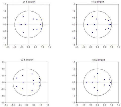
The stability of VAR model is the key factor and premise to judge whether it is a good model. The instability may cause the invalid analysis of ECM estimation, pulse response analysis and variance decomposition. The condition of the stability of VAR model is that all the equation root of the characteristic equation is less than 1, that is, all the reciprocals of equation roots model are within the circle.
Figure 1. AR equation root chart of each VAR model when lag phase is the second stage
The test results show that among the four VAR models, the model is steady when all the reciprocals of equation roots model are within the circle if the lag phase is the first or second stage. Figure describes the AR equation root charts of each VAR model when lag phase is the second stage. However, when the lag phase is more than the second stage, some the reciprocals of equation roots model are outside the circle. The conclusion can be gotten that in the premise of the steady VAR model, the primarily selected lag phase of the four VAR models is the first stage or the second one.
3.2 Causality test of VAR Granger
Causality test of VAR Granger is used to test whether the endogenous variable can be treated as the exogenous variable. If the equation of VAR model is involved in the empirical test, the causality test of VAR Granger must be used to confirm the mutual interpretation of each variable. Therefore, in order to verify whether the variables of border trade including the export and import can interpret the industrial structure alteration and whether the interpretation of the overall model is strong or not, the thesis conducts the causality test of VAR Granger of the four VAR models. In consideration that VAR model is steady when the lag phase is in the first and the second stage, the thesis conducts the causality test of VAR Granger when the lag phase is in the first and the second stage. Table 1 shows the result of the causality test of VAR Granger when the lag phase is in the second stage.
Table 1. VAR Granger causality test result
|
dependent variables |
lagged variables |
lag phase |
statistics |
df |
P value |
conclusion |
|
y1 |
dexport |
2 |
3.169 |
2 |
0.034 |
Y |
|
All |
29.087 |
12 |
0.001 |
Y |
||
|
dimport |
6.007 |
2 |
0.050 |
Y |
||
|
All |
23.115 |
12 |
0.010 |
Y |
||
|
y2 |
dexport |
2 |
1.290 |
2 |
0.086 |
N |
|
All |
27.090 |
12 |
0.008 |
Y |
||
|
dimport |
5.322 |
2 |
0.070 |
N |
||
|
All |
41.735 |
12 |
0.000 |
Y |
3.3 Residual examination of the model
Except for stability and the mutual interpretation among the variables, AR model should be tested by the residual examination so as to make sure the test result meet the classic hypothesis of VAR model, that is, random disturbance term has no autocorrelation and heteroscedasticity, as well as presents normal distribution.
Table 2. Model VAR residual examination test result
|
variables |
autocorrelation test |
|||||
|
y1 & dexport |
lag phase |
1 |
2 |
3 |
4 |
5 |
|
LM statistics |
56.057 |
41.829 |
36.027 |
34.491 |
26.730 |
|
|
P value |
0.058 |
0.233 |
0.467 |
0.540 |
0.869 |
|
|
J-B normality test |
statistics χ2=138.140 P value=0.993 |
|||||
|
White test for heteroscedasticity |
statistics χ2=521.217 P value=0.289 |
|||||
|
y1 & dimport |
lag phase |
1 |
2 |
3 |
4 |
5 |
|
LM statistics |
63.713 |
77.454 |
91.463 |
39.304 |
71.360 |
|
|
P value |
0.090 |
0.066 |
0.061 |
0.838 |
0.070 |
|
|
J-B normality test |
statistics χ2=184.990 P value =0.424 |
|||||
|
White test for heteroscedasticity |
statistics χ2=526.114 P value =0.240 |
|||||
|
y2 & dexport |
lag phase |
1 |
2 |
3 |
4 |
5 |
|
LM statistics |
60.618 |
55.462 |
54.015 |
50.465 |
37.719 |
|
|
P value |
0.056 |
0.051 |
0.067 |
0.055 |
0.391 |
|
|
J-B normality test |
statistics χ2=206.080 P value =0.107 |
|||||
|
White test for heteroscedasticity |
statistics χ2=523.278 P value =0.278 |
|||||
|
y2 & dimport |
lag phase |
1 |
2 |
3 |
4 |
5 |
|
LM statistics |
75.824 |
39.373 |
35.917 |
24.643 |
37.445 |
|
|
P value |
0.056 |
0.321 |
0.483 |
0.924 |
0.403 |
|
|
J-B normality test |
statistics χ2=188.526 P value =0.355 |
|||||
|
White test for heteroscedasticity |
statistics χ2=523.621 P value =0.274 |
|||||
Note: Cross terms are excluded in the test for heteroscedasticity.
When the residual examination is conducted, the Breusch-Godfrey LM test method is used to test the correlation; White’s test extended by Kelejian(1982)and Doornik(1995) to test heteroscedasticity, meanwhile, the J-B residual normality test method to test the normality of the residual. In order to avoid that the different results are caused by the covariance matrix orthogonalization method, the thesis adopts square root method of residual covariance matrix raised by Urzua(1997) to test the normality test of J-B residual error.
When the lag phase is in the second stage, the result of the residual examination test meets the classic hypothesis of the four VAR models residual, which is described in table 3. From the table 2, the residual of VAR model is below the significance level, that is, 5%, moreover, random disturbance term has no autocorrelation and heteroscedasticity, as well as presents normal distribution.
The four VAR models can have the stability, and pass the causality test of VAR Granger and the residual classic hypothesis test. Therefore, the best lag phase of the four VAR models is the second stage.
In the following part, the effect of industrial structure of the border trade in short and long term will be estimated by the co-integration method of Johansen and ECM estimation method. The premise of co-integration method is the steady variables in VAR model, so the stability should be tested by the unit root test method in order to check our whether the variables in the model meet the requirements of the integral in the same order.
4.1 The stability test of the variables
The data used in this thesis is the time series data. In order to avoid that some variables may have strong temporal trend which cause the variables to be unsteady, the thesis adopts the proportion form to measure the variables. The stability of the variables must be tested by the unit root test, so the spurious regression because of the unsteady variables can be avoided. The unit root test method this thesis adopts is Augmented Dickey -Fuller Test method raised by Dickey and Fuller (1981), and the selection standard of the best lag phase is AIC criterion and SC criterion. Whether the intercept term and trend term is included in the model can be figured out by the variables and the sequence chart of difference in certain order. The ADF test result of each variable and the sequence chart of the first order difference are presented in table 3.
Table 3. ADF unit root test result
|
variables |
test modality (c ,t ,n) |
ADF value |
P value |
critical value |
conclusion |
|
|
α=5% |
α=10% |
|||||
|
y1 |
(c ,t ,1) |
-1.468 |
0.815 |
-3.595 |
-3.233 |
unsteady |
|
y2 |
(0 ,0 ,0) |
-1.742 |
0.078 |
-1.954 |
-1.610 |
unsteady |
|
pgdp |
(c ,t ,4) |
-3.032 |
0.553 |
-3.632 |
-3.255 |
unsteady |
|
employ |
(c ,0 ,0) |
-1.873 |
0.079 |
-1.954 |
-1.610 |
unsteady |
|
wage |
(c ,t ,0) |
-3.418 |
0.498 |
-3.588 |
-3.239 |
unsteady |
|
fixasset |
(c ,t ,1) |
-1.783 |
0.684 |
-3.595 |
-3.233 |
unsteady |
|
dexport |
(c,t ,0) |
-3.006 |
0.572 |
-3.588 |
-3.229 |
unsteady |
|
dimport |
(c,t ,0) |
-3.999 |
0.151 |
-3.588 |
-3.229 |
unsteady |
|
△y1 |
(0 ,0 ,0) |
-3.397 |
0.002 |
-1.954 |
-1.609 |
steady |
|
△y2 |
(0 ,0 ,0) |
-9.769 |
0.000 |
-1.954 |
-1.609 |
steady |
|
△pgdp |
(c ,t ,2) |
-3.301 |
0.038 |
-1.958 |
-1.609 |
steady |
|
△employ |
(0 ,0 ,2) |
-4.484 |
0.000 |
-1.956 |
-1.609 |
steady |
|
△wage |
(0 ,0 ,0) |
-3.691 |
0.000 |
-1.954 |
-1.609 |
steady |
|
△fixasset |
(0 ,0 ,0) |
-3.953 |
0.005 |
-1.954 |
-1.609 |
steady |
|
△dexport |
(0 ,0 ,0) |
-5.949 |
0.000 |
-1.954 |
-1.609 |
steady |
|
△dimport |
(0 ,0 ,1) |
-5.208 |
0.000 |
-1.955 |
-1.609 |
steady |
In table 3, the ADF value is more than the significance critical value, that is, 5%, which means all the values have the unit root. However, the P value of each variable is less than 0.05 after the variable is tested by the first order difference, which means that under the significance level, that is, 5%, the sequence has no unit root, in other words, is the steady sequence. All the variables of four AVR model are the first order integration sequence, which meets the premise of the co-integration test.
4.2 The long-term equilibrium of the industrial structure
Granger raised the co-integration concept in 1981, which can be used to study whether the unsteady time sequence has the long-term equilibrium relationship. The unit root test result shows that the variables of four VAR model meet I(1), therefore, the thesis adopts multivariable co-integration test raised by Johansen and Juselius(1990)to test the long-term equilibrium relationship to measure whether there is the long-term equilibrium relationship among the variables. Because the co-integration test is used to test the first order difference of the variables, and the best lag phase for unrestraint VAR model is the second stage, the best lag phase for the co-integration test is the first stage. Table 4 is the co-integration test result of each VAR model when the lag phase is in the first stage. Co-integration equation (1) and (2) is the test result when the dependent variable is y1; Co-integration equation (3) and (4) is the test result when the dependent variable is y3.
Table 4. Long term effect of the industrial structure of the border trade
|
variables |
y1 |
y2 |
||
|
Co-integration equation (1) |
Co-integration equation (2) |
Co-integration equation (3) |
Co-integration equation (4) |
|
|
dexport |
-0.113*** |
|
0.018** |
|
|
(-13.987) |
|
(3.126) |
|
|
|
dimport |
|
-0.307 |
|
0.012** |
|
|
(-1.061) |
|
(3.369) |
|
|
pgdp |
-0.088*** |
-3.339*** |
-0.105*** |
-0.009 |
|
(3.793) |
(-3.551) |
(-4.623) |
(-0.564) |
|
|
employ |
1.707*** |
1.333*** |
3.541*** |
1.841*** |
|
(-4.934) |
(8.109) |
(6.581) |
(6.051) |
|
|
wage |
-0.192*** |
-6.815*** |
-0.065*** |
-0.054*** |
|
(15.283) |
(-11.334) |
(-4.485) |
(-5.022) |
|
|
fixasset |
0.054*** |
3.915*** |
0.005 |
0.053*** |
|
(5.457) |
(8.393) |
(0.415) |
(5.930) |
|
|
constant term |
16.705*** |
50.050*** |
5.089*** |
3.759*** |
|
|
|
(5.001) |
(3.811) |
|
|
co-integration test result |
|
|
|
|
|
None |
186.161*** |
164.281*** |
136.317*** |
121.732*** |
|
[0.000] |
[0.000] |
[0.000] |
[0.002] |
|
|
At most 1 |
117.166*** |
103.636*** |
85.574*** |
78.722** |
|
[0.000] |
[0.004] |
[0.010] |
[0.037] |
|
|
At most 2 |
64.042*** |
67.771** |
45.719 |
51.264* |
|
[0.007] |
[0.023] |
[0.224] |
[0.087] |
|
According to the measurement method of dependent variable y1 and y2, y1 stands for the proportion of the added value of the secondary industry, which can reflect the direction of the industrial structure; while, y2 stands for the coefficient of variation of the industrial structure, which reflects the industrial structure has changed or not. In the following part, the thesis firstly analyzes the co-integration test result when the dependent variable is y2, that is, the result of co-integration equation (3) and (4), so as to study whether the development of border trade has impact on the industrial structure alteration. If the coefficient of dexpor tand dimport is positive, it means the export and import of border trade has impact on the industrial structure alteration; if it is negative, it means the export and import of border trade represses the industrial structure alteration; if the estimation result is not significant, it means there is no correlation between the border trade and the industrial structure alteration. The thesis further analyzes the estimation result when the dependent variable is y1 to study the direction of the impact of border trade on the industrial structure alteration. If the coefficient of dexpor tand dimport is positive, it means the industrial structure alteration is mainly caused by the secondary industry; if it is negative, it means the increasing proportion of the tertiary industry is the major factor to cause the effect of the industrial structure of border trade.
Based on the co-integration test result in table 4, four VAR models have the co-integration relationship. Co-integration equation (1) and (2) has three co-integration relationships; co-integration equation (3) and (4) has two co-integration relationships; those co-integration relationships can be presented as the co-integration equations in table 4.
In co-integration equation (3), the dexport coefficient of border export is 0.018, and over the significance level test, that is, 5%, which means the border export in Inner Mongolia can cause the industrial structure alteration, moreover, has the significant impact on it. In co-integration equation (4), the dimport coefficient of border export is 0.012, and over the significance level test, that is, 5%, which means the border import in Inner Mongolia can has the significant impact on the industrial structure alteration and the effect of border import on the industrial structure alteration is less than the one of border export. The direction of the industrial structure alteration caused by border trade, the estimation result of co-integration equation (1) shows that the coefficient of dexport is -0.113, which means the effect of border export trade on the industrial structure alteration is mainly on the decrease proportion of the secondary industry and the increase proportion of the tertiary industry, meanwhile, reflects that the border export is helpful to speed up the industrialization and the development of other service industry. In co-integration equation (2), the coefficient of dimport is negative, but not significant, which means direction of the effect of border import on the industrial structure is the same as the border export. However, in the long term, its impact is not significant.
The border export can have more impact on the industrial structure alteration, which mainly reflects on decreasing the proportion of the secondary industry and increasing the tertiary industry; the border import can have less impact on the industrial structure alteration, and the direction of the effect of border import on the industrial structure is the same as the border export. However, the impact is not so significant.
As for the effect of the control variables, the effect of PGDP which measures the economic development level on the industrial structure alteration is negative, which mainly because the amount of variation of the industrial structure alteration began to flatten with the development of the economy in certain country or region. From the view of direction of the industrial structure alteration, the coefficients of co-integration equation (1) and (2) are negative which means the higher the economic development level, the industrial structure tends to the servitization. Such trend is accordance with the one in developed countries all over the world. According to the data delivered by World Bank Database, the added value proportion of service industry has reached up to more than 70%. The effect of employ variable on the industrial structure alteration is positive, which means the alteration of the employment structure can cause the significant alteration of the industrial structure. Moreover, the direction of the industrial structure alteration is the same as the one of employment structure, because the coefficients of employ in co-integration equation (1) and (2) are positive. Such phenomena are accordance with the practical condition. In the industrial structure, the larger the added values proportion of the secondary and the tertiary industry, the stronger the ability of employment, and vice-versa. The wage variable in the four co-integration equations is negative, which shows that, on the one hand, the increase of the wage level in certain region can cause that the industrial structure alteration begins to flatten, which is the same as the effect of the industrial structure alteration of the economic development level. It is mainly because the increase of the wage level means the higher economic development level; on the other hand, the increase of wage level can cause the proportion of the secondary industry decreases, meanwhile, the proportion of the tertiary industry in the industrial structure increase, which means the increase of wage level tend to servitization. The effect of fixasset variable on the industrial structure is positive, which means the increase of the fix-asset investment can cause the industrial structure alteration to some extent. Moreover, the coefficients of fixasset in co-integration equation (1) and (2) are positive, which shows that the increase of the fix-asset investment can cause the proportion of the secondary industry increase in the industrial structure, that is, restrain the servitization. The main reason of such phenomenon is that the production of the secondary industry demands more fix-asset investment volume, while, the production of the serving products need less fix-asset investment volume.
Such conclusion can be gotten that the border export can have more impact on the industrial structure alteration, which mainly reflects on decreasing the proportion of the secondary industry and increasing the tertiary industry; the border import can have less impact on the industrial structure alteration, and the direction of the effect of border import on the industrial structure is the same as the border export. However, the impact is not so significant.
[1] Lan Qingxin and Tian Haifeng, “Substantial evidence analysis and present situation research on trade structure change and economic growth model transformation in China”, Journal of Zhuzhou Institute of Technology, vol. 3, pp. 39-44, 2002.
[2] Dickey, D. and W. Fuller, “Likelihood ratio tests for autoregressive time series with a unit root”, Econometria, vol. 49, no. 4, pp. 1057-1073, 1981.
[3] Granger, C. W. J., “Some properties of time series data and their use in econometric model specification”, Journal of Econometrics, vol. 16, no. 1, pp. 121-130, 1981.
[4] Johansen, S. and Juselius, K., “Maximum likelihood estimation and inference on cointegration- with applications to the demand for money”, Oxford Bulletin of Economics and Statistics, vol. 52, no. 2, pp. 169-210, 1990.
[5] Kelejian, H. H., “An extension of a standard test for heteroscedasticity to a systems framework”, Journal of Econometrics, vol. 20, no. 2, pp. 325-333,1982.
[6] Lutkepohl, H., Introduction to Multiple Time Series Analysis, New York: Springer-Verlag, 1991.
[7] Urzua, C. M., “Omnibus tests for multivariate normality based on a class of maximum entropy distributions”, in Advances in Econometrics, vol. 12, Greenwich, Conn.: JAI Press, pp. 341-358, 1997.