Priscila Ortega*![]() | Zoe Infante
| Zoe Infante![]() | Carlos F. Ortiz
| Carlos F. Ortiz![]()
© 2024 The authors. This article is published by IIETA and is licensed under the CC BY 4.0 license (http://creativecommons.org/licenses/by/4.0/).
OPEN ACCESS
This study aims to evaluate and analyze global sustainability over three decades, from 1990 to 2020. To achieve this, a sustainability index was constructed based on the underlying theories of the concept, using representative indicators of its three dimensions: environmental, social, and economic. The data were processed using the Stata software. The results show that the global sustainability index has had an upward trend, although with some setbacks in certain periods, such as between 2004 and 2007. In the last five years, there has been a consistent increase in the index, with 2020 standing out with a significantly higher value compared to previous years. It is concluded that the combined efforts of various international organizations, along with the policies implemented by countries, have been crucial in improving the level of global sustainability.
sustainability index, social dimension, economic dimension, environmental dimension
Global sustainability has emerged as a central theme in political, economic, and environmental agendas over the past decades. With the growing recognition of the environmental, social, and economic challenges facing our planet, the need to assess and improve sustainability has become imperative. From the Earth Summit in Rio de Janeiro in 1992 to the United Nations Sustainable Development Goals established in 2015, there has been a continuous and coordinated effort to promote sustainable practices globally.
The period from 1990 to 2020 has witnessed significant changes and developments in how nations approach sustainability. During these three decades, numerous policies and strategies have been implemented to balance economic growth with environmental protection and social equity. However, despite the progress made, significant challenges persist that require ongoing attention and concerted efforts.
This research aims to evaluate and analyze global sustainability over these three decades. To achieve this, a sustainability index has been constructed, integrating indicators from the three dimensions of sustainability: environmental, social, and economic. This index provides a comprehensive measure of global sustainability performance, allowing for the identification of trends, advancements, and setbacks over time.
The analysis of the data, processed using Stata software, reveals crucial trends in the evolution of global sustainability. The results obtained not only offer a detailed view of the progress made but also highlight periods where setbacks occurred. In particular, the study emphasizes the notable increase in the sustainability index over the past five years, culminating in a significantly higher value in 2020 compared to previous years.
This study underscores the importance of the combined efforts of international organizations and national policies in improving global sustainability. This research not only provide a deeper understanding of the dynamics of global sustainability but also offer valuable lessons for future policies and strategies aimed at achieving sustainable development.
2.1 Sustainability
Sustainability is a concept that has evolved over time, reflecting changes in how societies perceive their relationship with the environment, the economy, and social well-being. Although today it is associated with the balance between these three dimensions, its meaning and application have been the subject of debate among academics, policymakers, and private sector actors.
Throughout history, various theories have emerged to explain how to achieve sustainable development. However, is it truly possible to balance economic growth with environmental conservation? Is sustainability an achievable goal or merely a regulatory aspiration? These questions are key to the discussion on the future of global development.
One of the most significant milestones in the evolution of the concept of sustainability was the Brundtland Report [1], published by the UN's World Commission on Environment and Development. This report defined sustainable development as:
"Development that meets the needs of the present without compromising the ability of future generations to meet their own needs" [1].
This definition laid the foundation for modern sustainability and established the idea that development cannot rely solely on economic growth but must also consider environmental and social impacts.
Since then, the discussion has focused on whether economic growth can be compatible with sustainability. On one hand, the Green Growth perspective argues that economic growth and sustainability are not mutually exclusive but can complement each other through efficient resource use, clean technologies, and innovation [2]. On the other hand, the Limits to Growth perspective contends that infinite economic growth is unsustainable due to the planet's limited capacity to absorb environmental impacts [3].
The Limits to Growth theory [3] originated from the Club of Rome's report. It argues that unlimited economic growth is unsustainable due to the planet's physical constraints.
Thus, the concept of sustainable development emerges as a paradigm that encourages reflection on the consequences of development, integrating three dimensions: economic, ecological, and socio-cultural redirecting us towards greater socioeconomic development, which translates into a better quality of life for all [4-6].
Thus, sustainable development is a development model with a shared, holistic, and long-term vision that countries have agreed upon as the best way to improve people's lives worldwide; promoting prosperity and economic opportunities, greater social well-being, and environmental protection [7].
Sustainability is associated with the transformation of social, economic, and environmental spheres in which humans evolve, with the purpose of meeting present and future needs under strategies developed for this purpose [8].
The economic dimension refers to the productive capacity and economic potential of rural territories to generate the necessary goods and wealth for the present and future of their inhabitants [9]. The environmental dimension is defined as the capacity of a system to maintain its state over time, conserving the parameters of volume, rate of change, and circulation invariability, or cyclically fluctuating these parameters around average values [10, 11].
The social dimension is achieved when costs and benefits are distributed adequately and equitably both among the current population (intragenerational equity) and between present and future generations (intergenerational equity). It requires incorporating the notion of quality of life. Many researchers and international organizations measure a nation's social development by evaluating the satisfaction of basic natural needs [10, 11].
Government policies play an important role in advancing sustainability. The presence of a correlation between the dimension of governance and the success of sustainability has been empirically confirmed [12].
2.2 Theoretical discussion on Principal Component Analysis (PCA)
Principal Component Analysis (PCA) is one of the most widely used statistical techniques for dimensionality reduction and exploratory analysis of multivariate data. Its origins date back to Pearson [13], who introduced the idea of representing a dataset in a lower-dimensional space through orthogonal projection onto principal axes. Later, Hotelling [14] formalized PCA from an algebraic perspective, founded upon the eigenvalue decomposition of the covariance matrix.
PCA has become a fundamental tool in various disciplines, such as biology, econometrics, and machine learning [15]. In data mining and pattern recognition, it is used to reduce dimensionality without losing essential information [16]. Additionally, it is applied in economics and social sciences for analyzing composite indicators and detecting relationships between variables [17].
In genetics, PCA is used to identify population structure and genetic variations across individuals [18]. In finance, it helps in portfolio optimization by reducing the dimensionality of correlated assets, thereby improving risk management strategies [19]. Moreover, in image processing and computer vision, PCA plays a crucial role in facial recognition and compression techniques [20].
Several studies have applied PCA to sustainability research, demonstrating its versatility in analyzing complex environmental and socio-economic data.
Yengle Ruiz [21] employed PCA to transform simple environmental quality indicators into composite indices in the La Libertad department. He identified three main components related to household quality of life, environmental temperature, and external environmental quality.
In the project called “Análisis espacial del Índice de Sustentabilidad Ambiental Urbana en la Megalópolis de México” was created using PCA, evaluating 189 municipalities through 17 standardized indicators [22].
In the study named “Post-Harvest Pineapple Quality Monitoring”, Fernández-Chuairey et al. [23] employed PCA to assess quality parameters such as weight loss, firmness, color index, and pH, explaining 88.36% of the variance in the data.
Polanco Martínez [24] explores the use of Principal Component Analysis (PCA) in evaluating air quality monitoring networks. The author applies this statistical technique to analyze data collected by various air quality monitoring stations, aiming to identify patterns in pollution levels across different areas.
Mathematical Foundations of PCA
PCA is based on transforming a set of original variables into a new set of uncorrelated variables called principal components. These components are obtained through the spectral decomposition of the covariance or correlation matrix, depending on whether the variables are on different scales [25]. The first principal component captures the highest possible variance in the data, and subsequent components successively explain the remaining variability while being orthogonal to each other [26].
Mathematically, if X is a centered data matrix, PCA is obtained from the eigenvalue decomposition of its covariance matrix:
$S=\mathbf{V} \Lambda \mathbf{V}^T$ (1)
where:
• V contains the eigenvectors, which define the new coordinate system (principal components).
• Λ (Lambda) is a diagonal matrix with eigenvalues, representing the variance explained by each principal component.
• ${V}^T$ (transpose of V) ensures the reconstruction of S through the transformation.
One important aspect of PCA is the percentage of variance explained (PVE) by each principal component, which helps determine how many components should be retained in the analysis. This is typically done by examining the scree plot, where a significant drop in eigenvalues suggests an appropriate cutoff point [27].
Interpretation of Principal Components
Each derived component is formulated as a linear aggregation of the initial variables, and their coefficients (known as loadings) indicate how much each variable contributes to a given component. Large absolute values of loadings suggest strong associations between the principal component and the original variables [28].
A common approach to enhance interpretability is to apply varimax rotation, which maximizes the variance of squared loadings, making the components more distinct and easier to interpret [29]. This is especially useful in fields like psychology and social sciences, where PCA is used for factor extraction in exploratory factor analysis (EFA).
To achieve the objective of the present research, the following steps were carried out:
1. Definition of the objective of the global sustainability index.
Evaluate and analyze global sustainability trends across three decades, from 1990 to 2020, focusing on key indicators in economic, social, and environmental dimensions.
2. Determination of the dimensions: Economic, Social, and Environmental.
3. Selection of Indicators and their classification: Eleven representative indicators of the three dimensions (environmental, social, and economic) were selected for the period 1990-2020:
-GDP per capita: Measures the economic output per person.
-Gross national income (GNI) per capita. Accounts for income from abroad.
-Proportion of the total labor force that is unemployed, based on ILO modeled estimates). Indicates the percentage of the labor force that is unemployed, reflecting economic health.
-Incidence of poverty at the societal poverty line, expressed as a percentage of the total population. Poverty is often tied to economic factors such as income distribution.
-Life expectancy at birth. Reflects the overall health and longevity of a population, an indicator of social well-being.
-Expected years of schooling. Measures access to education, a key social development indicator.
-Mean years of schooling. this measures educational attainment.
-CO2 emissions (kt). An indicator of environmental impact, specifically in terms of greenhouse gas emissions.
-Renewable energy consumption (% of total final energy consumption). Environmental (but with economic implications): Although environmental in nature, renewable energy adoption also affects economic sustainability.
-Earth's surface temperature variation ℃ (Meteorological year). Reflects climate change, a key environmental concern.
-Adjusted savings: education expenditure (% of GNI). Although primarily related to education, it shows the level of investment in human capital.
Political (or Governance-related): No direct political indicators were considered, but some of the economic and social variables may reflect the political climate in a country, such as policies on education, unemployment, and renewable energy.
4. Data Collection: Information sources: World Bank and United Nations.
5. Data Standardization: The variables were standardized using the Z-score method to transform the data so that they have a mean of 0 and a standard deviation of 1. This is done to make data from different scales comparable. The standardization process is performed using the following formula:
$\mathrm{Z}=\frac{\chi-\mu}{\sigma}$ (2)
where:
Ζ is the standardized value.
$\chi$ is the original value.
μ is the mean of the data set.
σ is the standard deviation of the data set.
6. Weight Assignment: The principal component analysis (PCA) technique was used for this. It uses the loadings of the principal components to calculate the weights of each variable.
Calculation of the Sustainability Index: For this, the weighted normalized indicators were aggregated to obtain a composite value for each dimension, and the weighted dimensions were combined to calculate the overall sustainability index:
Sustainability Index $=\sum_{i=1}^n\left(w_i \cdot x_1^{\prime}\right)$ (3)
where, $w_i$ is the weight assigned to the indicator and $x_1^{\prime}$ is the normalized value of indicator $i$.
7. Finally, the results are interpreted.
For the principal component analysis, 11 components were extracted, which is equal to the number of original variables. The eigenvectors table shows the loadings of each original variable on the principal components. These loadings indicate the contribution of each variable to the component and can be interpreted as coefficients in a linear combination.
Table 1. Eigenvalue
|
Component |
Eigenvalue |
Difference |
Proportion |
Cumulative |
|
Comp1 |
8.47839 |
7.35814 |
0.7708 |
0.7708 |
|
Comp2 |
1.12025 |
0.315333 |
0.1018 |
0.8726 |
|
Comp3 |
0.804921 |
0.360109 |
0.0732 |
0.9458 |
|
Comp4 |
0.444811 |
0.309181 |
0.0404 |
0.9862 |
|
Comp5 |
0.135631 |
0.127691 |
0.0123 |
0.9985 |
|
Comp6 |
0.00794018 |
0.00390798 |
0.0007 |
0.9993 |
|
Comp7 |
0.0040322 |
0.00204331 |
0.0004 |
0.9996 |
|
Comp8 |
0.00198889 |
0.000631495 |
0.0002 |
0.9998 |
|
Comp9 |
0.00135739 |
0.000782857 |
0.0001 |
0.9999 |
|
Comp10 |
0.000574536 |
0.000478168 |
0.0001 |
1.0 |
|
Comp11 |
9.63679E-05 |
0.0 |
1.0 |
Source: Authors’ design in Stata program based on World Bank and ONU data.
Component 1 has an eigenvalue of 8.47839, which means it explains a large proportion of the total variance (77.08%). The cumulative variance after the first component is also 77.08%.
Component 2 explains an additional 10.18% of the variance, bringing the cumulative variance to 87.26%. Component 3 explains another 7.32%, bringing the cumulative variance to 94.58%, which is sufficient to capture most of the information from the original data (see Table 1).
Component 1 contains eight variables with similar loadings around ±0.34. This suggests that this component is an almost equal combination of all these variables, capturing a general dimension of the data.
Component 2 contains two variables with significant loadings: renewable energy consumption, with a negative sign, and education expenditure, with a positive sign.
Unemployment rate shows a higher loading in Component 3 than in Component 2.
Some variables considered in Component 1 show higher loadings in other components; however, it is more beneficial to consider them in Component 1 despite their lower loadings because it is much more relevant in terms of the explained variance (see Table 2).
Table 2. PC of sustainability
|
Variable |
Comp1 |
Comp2 |
Comp3 |
|
z_poverty |
-0.3394 |
-0.1019 |
0.04 |
|
z_leb |
0.34 |
0.1017 |
-0.0676 |
|
z_eys |
0.3386 |
0.0986 |
-0.1015 |
|
z_ays |
0.341 |
0.0672 |
0.0716 |
|
z_GNI |
0.3388 |
0.0112 |
-0.1604 |
|
z_GDPPC |
0.3406 |
0.0283 |
-0.1209 |
|
z_eCO2 |
0.3331 |
0.1455 |
-0.1876 |
|
z_REC |
0.1491 |
-0.6794 |
0.4466 |
|
z_ESTV |
0.3166 |
-0.1053 |
0.0159 |
|
z_EE |
-0.2227 |
0.5365 |
-0.008 |
|
z_Unemp |
0.1563 |
0.427 |
0.8385 |
Source: Authors’ design in Stata program based on World Bank and ONU data.
Table 3. Variable weights
|
Variable |
Sum_abs_Loadings |
Weight |
|
z_ poverty |
0.4813 |
0.0635178 |
|
z_leb |
0.5093 |
0.067213 |
|
z_eys |
0.5387 |
0.071093 |
|
z_ays |
0.4798 |
0.0633199 |
|
z_GNI |
0.5104 |
0.0673582 |
|
z_GDPPC |
0.4898 |
0.0646396 |
|
z_eCO2 |
0.6662 |
0.0879193 |
|
z_REC |
1.2751 |
0.1682767 |
|
z_ESTV |
0.4378 |
0.0577771 |
|
z_EE |
0.7672 |
0.1012485 |
|
z_Unemp |
1.4218 |
0.1876369 |
Note: abs (): represents the sum of the absolute values of the components: Comp1, Comp2, and Comp3. Sum_abs_loadings: reflects the relative contribution of each variable based on its loadings in the principal components.
Source: Authors’ design in Stata program based on World Bank and ONU data.
To obtain the weights of each variable, the absolute loadings of the first three selected components are summed, using the weights obtained from PCA to calculate the index (see Table 3).
The variables with the greatest weight are Unemployment (z_Unemp), Renewable Energy Consumption (z_REC), Education Expenditure (z_EE), CO2 Emissions (z_eCO2).
The results of the sustainability index vary from -0.0121157 (1990) to 0.0125372 (2020). These values indicate that some periods or data points have higher (positive) sustainability indices while others have lower (negative) indices (see Table 4).
Table 4. World sustainability index
|
Year |
World Sustainability Index |
Year |
World Sustainability Index |
|
1990 |
-0.0121157 |
2006 |
-0.0003245 |
|
1991 |
-0.0115007 |
2007 |
-0.0011179 |
|
1992 |
-0.0086443 |
2008 |
-0.0006468 |
|
1993 |
-0.0071932 |
2009 |
0.0034052 |
|
1994 |
-0.0044001 |
2010 |
0.0027813 |
|
1995 |
-0.0041022 |
2011 |
0.0028142 |
|
1996 |
-0.003893 |
2012 |
0.0028297 |
|
1997 |
-0.0023772 |
2013 |
0.0048195 |
|
1998 |
-0.0023751 |
2014 |
0.0053437 |
|
1999 |
-0.0013549 |
2015 |
0.0045728 |
|
2000 |
-0.0020322 |
2016 |
0.0046557 |
|
2001 |
-0.0012872 |
2017 |
0.0053203 |
|
2002 |
0.0006587 |
2018 |
0.0052912 |
|
2003 |
0.001626 |
2019 |
0.0064932 |
|
2004 |
0.0002994 |
2020 |
0.0125372 |
|
2005 |
-8.3E-05 |
|
|
Source: Authors’ design in Stata program based on World Bank and ONU data.
For better understanding of the results, the index was normalized with values from zero to one. 0 corresponds to the lowest value of the original index (-0.012116 in 1990), and 1 corresponds to the highest value of the original index (0.012537 in 2020). Intermediate values are proportionally scaled between these two extremes.
Table 5. Normalized sustainability index
|
Year |
Sustainability_Index_Norm |
Year |
Sustainability_Index_Norm |
|
1990 |
0.0 |
2006 |
0.478319 |
|
1991 |
0.02496 |
2007 |
0.446112 |
|
1992 |
0.140835 |
2008 |
0.465217 |
|
1993 |
0.199692 |
2009 |
0.629579 |
|
1994 |
0.312984 |
2010 |
0.604267 |
|
1995 |
0.325072 |
2011 |
0.605606 |
|
1996 |
0.33355 |
2012 |
0.606255 |
|
1997 |
0.395043 |
2013 |
0.686935 |
|
1998 |
0.395124 |
2014 |
0.70823 |
|
1999 |
0.436499 |
2015 |
0.676956 |
|
2000 |
0.409037 |
2016 |
0.680323 |
|
2001 |
0.439257 |
2017 |
0.707257 |
|
2002 |
0.518193 |
2018 |
0.70608 |
|
2003 |
0.557417 |
2019 |
0.754837 |
|
2004 |
0.50359 |
2020 |
1.0 |
|
2005 |
0.488095 |
Source: Authors’ design in Stata program based on World Bank and ONU data.
Table 5 shows a general trend of increase in the sustainability index over time. A gradual growth is observed from 0.0 in 1990 to 1.0 in 2020. Although the overall trend is upward, there are fluctuations in some years. For example, in 2007, the index decreases to 0.446112 compared to 2006 (0.478319), but then rises again in the following years. It can be noted that in certain periods the index increases more rapidly. For example, between 2009 and 2013, there is a notable increase from 0.629579 to 0.686935 (see Table 5).
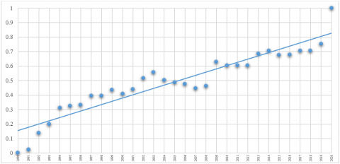
Figure 1 shows the evolution of the Normalized Sustainability Index from 1990 to 2020. The trend line (in blue) indicates a clear upward trend over time, suggesting a general improvement in the sustainability index during the analyzed period. The dispersion of points around the trend line shows annual variations in the index. The trend line provides an overview of the change in the sustainability index over time, smoothing out annual fluctuations. The positive slope of the trend line confirms an improvement in sustainability levels. This improvement can be attributed to various policies, practices, and conditions that have favored sustainable development over time.
Figure 1. Evolution of the normalized sustainability index
4.1 Discussions
The performance of each variable in the sustainability index is determined by the weights assigned to each one. The weights reflect the relative importance of each variable in contributing to the overall index.
Variables with High Weights (Greater Influence)
Unemployment has the highest weight, meaning it has the greatest influence on the sustainability index. A high unemployment rate can significantly decrease the sustainability index, indicating economic and social issues. Conversely, a low unemployment rate can increase the index, reflecting a healthier economy and better social well-being.
Renewable energy consumption also has a high weight. Higher consumption of renewable energy indicates more sustainable development, reducing dependence on fossil fuels and lowering greenhouse gas emissions, which would improve the sustainability index.
Education expenditure has a significant weight. Greater investment in education is often associated with positive socioeconomic development, improving the employment and economic prospects of the population, which would increase the sustainability index.
Variables with Moderate Weights
CO2 emissions have a moderate weight. High CO2 emissions can reduce the sustainability index, indicating a negative environmental impact. Reductions in emissions would improve the index, reflecting greater environmental responsibility.
Life expectancy at birth is a key indicator of the health and well-being of the population. An increase in life expectancy is generally associated with better living conditions and more efficient health systems, which can improve the sustainability index.
Income per capita has a moderate impact on the index. Higher income per capita generally indicates a wealthier population with better access to resources and services, improving the sustainability index.
GDP per capita is an important indicator of a nation's wealth and economic well-being. A high GDP per capita can improve the sustainability index, reflecting a prosperous economy and better quality of life.
Variables with Low Weights (Lesser Influence)
The poverty rate has a relatively low weight. However, high levels of poverty can still negatively impact the sustainability index, reflecting socioeconomic inequalities.
Expected years of schooling has a lower but significant weight. A higher number of expected years of schooling can improve the index by indicating better future educational outcomes and human capital development.
Earth's surface temperature variation has the lowest weight. Although it is an important environmental indicator, its impact on the index is smaller compared to other indicators.
The Sustainability Index shows a clear upward trend from 1990 to 2020. This indicates a continuous improvement in sustainability levels during this period. The positive trend in the index can be attributed to the implementation of favorable policies, practices, and conditions that have promoted sustainable development. This includes environmental, social, and economic policies that have contributed to another improvement in key sustainability indicators. Although the overall trend is positive, there are annual fluctuations reflecting changes in the economic, social, and environmental conditions of each year. These variations may be due to factors such as economic crises, natural disasters, changes in government policies, among others.
Variables with higher weights have a greater influence on the sustainability index. This means that changes in these variables (such as unemployment, renewable energy consumption, and education) will have a larger impact on the overall index. Variables with lower weights, while less influential, still contribute to the index and should not be ignored in the assessment of sustainability. Life expectancy at birth, although with a moderate weight, remains a key indicator of the overall well-being of the population.
Some limitations of the Global Sustainability Index are: Aggregating data at a global level can obscure important regional or local trends; Interactions between economic, social, and environmental dimensions can be difficult to model in a single composite index; Some important subdimensions of sustainability may not be adequately captured; some dynamics may not be fully reflected if the indicators do not adequately capture changes in industrial practices, international policies, or technological innovations. Despite these limitations, such an index can provide valuable insights into global sustainability trends. However, the results should be interpreted cautiously and complemented with more detailed analyses to capture the complexity and dynamics of sustainability over time.
This study focused on measuring sustainability at a global level over two decades, analyzing the performance of key indicators in each dimension. However, future research could explore studies by groups of countries, whether by trade blocs, economic regions, continents, or similar characteristics, allowing for a more detailed understanding of sustainable dynamics in different contexts. Likewise, studies on the impact of sustainability strategies in specific sectors, such as organic agriculture or the manufacturing industry, could provide key insights for designing more effective policies.
|
z_ poverty |
The poverty rate at the societal poverty line (% of the population) |
|
z_leb |
Life expectancy at birth |
|
z_eys |
Expected years of schooling |
|
z_ays |
Average years of schooling |
|
z_GNI |
Gross national income (GNI) per capita |
|
z_GDPPC |
GDP per capita (constant 2015 US$) |
|
z_eCO2 |
CO2 emissions (kt) |
|
z_REC |
Renewable energy consumption (% of total final energy consumption) |
|
z_ESTV |
Earth's surface temperature variation ℃ (Meteorological year) |
|
z_EE |
Adjusted savings: education expenditure (% of GNI) |
|
z_Unemp |
Unemployment, total (% of total labor force) |
The data supporting the dimensions that comprise the sustainability index are available at:
https://hdr.undp.org/data-center/documentation-and-downloads
https://databank.worldbank.org/reports.aspx?source=2&series=SL.UEM.TOTL.ZS&country=
[1] World Commission on Environment and Development (WCED). (1987). Our common future (Brundtland report). New York. http://digitallibrary.un.org/record/139811.
[2] Organización para la Cooperación y el Desarrollo Económicos (OCDE). (2011). Towards Green Growth. OECD Publishing. https://doi.org/10.1787/9789264111318-en
[3] Meadows, D.H., Meadows, D.L., Randers, J., Behrens, W.W. (1972). The limits to growth: A report for the club of Rome's project on the predicament of mankind. Demography, 10(2): 289-295. https://doi.org/10.2307/2060819
[4] Garza, E.G. (2007). De las teorías del desarrollo al desarrollo sustentable. Historia de la construcción de un enfoque multidisciplinario. Trayectorias, 9(25): 45-60.
[5] Hernández Paz, A.A., González García, H., Tamez González, G. (2016). Desarrollo sustentable: de la teoría a la práctica. Estudios rurales en México, 113-140. https://doi.org/10.2307/j.ctvtxw358.8
[6] Instituto Nacional de Ecología (Mexico). (2000). Indicadores de desarrollo sustentable en México. Instituto Nacional de Ecología.
[7] United Nations. (2015). Transforming our world: The 2030 agenda for sustainable development. United Nations. https://sustainabledevelopment.un.org/content/documents/21252030%20Agenda%20for%20Sustainable%20Development%20web.pdf.
[8] Casas-Cázares, R., González-Cossío, F.V., García-Moya, E., Martínez-Saldaña, T., Peña-Olvera, B.V. (2008). Contribución de la dimensión ambiental al desarrollo sustentable de tres agroecosistemas campesinos. Terra Latinoamericana, 26(3): 275-284. https://www.scielo.org.mx/scielo.php?pid=S0187-57792008000300009&script=sci_arttext.
[9] Nieto Masot, A., Gurría Gascón, J.L. (2024). Sustainable Rural Development: Strategies, Good Practices and Opportunities (Second Edition). Land, 13(1): 104. https://doi.org/10.3390/land13010104
[10] Shaw, R.W., Gallopin, G.C., Weaver, P., Öberg, S. (1992). Sustainable Development: A Systems Approach. IIASA Status Report. IIASA, Laxenburg, Austria: SR-92-006. https://pure.iiasa.ac.at/id/eprint/3602/.
[11] López, I., Arriaga, A., Pardo, M. (2018). The social dimension of sustainable development: The everlasting forgotten? Revista Española de Sociología, 27(1): 25-41. https://doi.org/10.22325/fes/res.2018.2
[12] Glass, L.M., Newig, J. (2019). Governance for achieving the Sustainable Development Goals: How important are participation, policy coherence, reflexivity, adaptation and democratic institutions? Earth System Governance, 2: 100031. https://doi.org/10.1016/j.esg.2019.100031
[13] Pearson, K. (1901). LIII. On lines and planes of closest fit to systems of points in space. The London, Edinburgh, and Dublin Philosophical Magazine and Journal of Science, 2(11): 559-572. https://doi.org/10.1080/14786440109462720
[14] Hotelling, H. (1933). Analysis of a complex of statistical variables into principal components. Journal of Educational Psychology, 24(6): 417-441. https://doi.org/10.1037/h0071325
[15] Hastie, T., Tibshirani, R., Friedman, J.H., Friedman, J.H. (2009). The elements of Statistical Learning: Data Mining, Inference, and Prediction, pp. 1-758. New York: Springer. https://doi.org/10.1007/978-0-387-21606-5
[16] Bishop, C.M., Nasrabadi, N.M. (2006). Pattern Recognition and Machine Learning, p. 738. New York: springer.
[17] James, G., Witten, D., Hastie, T., Tibshirani, R. (2013). An Introduction to Statistical Learning with Applications in R. Springer. https://doi.org/10.1007/978-1-4614-7138-7
[18] Patterson, N., Price, A.L., Reich, D. (2006). population structure and eigenanalysis. PLoS Genetics, 2(12): e190. https://doi.org/10.1371/journal.pgen.0020190
[19] Alexander, C. (2001). Market Models: A Guide To Financial Data Analysis. University of Sussex. John Wiley & Sons.
[20] Turk, M., Pentland, A. (1991). Eigenfaces for Recognition. Journal of Cognitive Neuroscience, 3(1): 71-86. https://doi.org/10.1162/jocn.1991.3.1.71
[21] Yengle Ruiz, C. (2012). Aplicación del análisis de componentes principales como técnica para obtener índices sintéticos de calidad ambiental. UCV-Scientia, 4(2): 145-153. https://revistas.ucv.edu.pe/index.php/ucv-scientia/article/view/952.
[22] De Las Heras Gutiérrez, D., Adame Martínez, S., Cadena Vargas, E.G., Campos Alanís, J. (2020). Análisis espacial del Índice de Sustentabilidad Ambiental Urbana en la Megalópolis de México. Investigaciones Geográficas, (73): 147–169. https://doi.org/10.14198/INGEO2020.HGAMCVCA
[23] Fernández-Chuairey, L., Rangel-Montes de Oca, L., Varela-Nualles, M., Pino-Roque, J.A., del Pozo-Fernández, J., Lim-Chamg, N.U. (2022). Análisis de componentes principales, una herramienta eficaz en las Ciencias Técnicas Agropecuarias. Revista Ciencias Técnicas Agropecuarias, 31(1).
[24] Polanco Martínez, J.M. (2016). The role of principal component analysis in the evaluation of air quality monitoring networks. Comunicaciones en Estadística, 9(2): 271-294. https://doi.org/10.15332/s2027-3355.2016.0002.06
[25] Jolliffe, I.T. (2002). Principal Component Analysis, Second Edition. Springer. http://cda.psych.uiuc.edu/statistical_learning_course/Jolliffe%20I.%20Principal%20Component%20Analysis%20(2ed.,%20Springer,%202002)(518s)_MVsa_.pdf.
[26] Mardia, K.V., Kent, J.T., Bibby, J.M. (1979). Multivariate Analysis. Academic Press. https://statisticalsupportandresearch.wordpress.com/wp-content/uploads/2017/06/k-v-mardia-j-t-kent-j-m-bibby-multivariate-analysis-probability-and-mathematical-statistics-academic-press-inc-1979.pdf.
[27] Cattell, R.B. (2010). The scree test for the number of factors. Multivariate Behavioral Research, 1(2): 245-276. https://doi.org/10.1207/s15327906mbr0102_10
[28] Rencher, A.C. (2002). Methods of Multivariate Analysis (Second Edition). Wiley-Interscience. https://eprints.uad.ac.id/135/1/Handbook_of_analysis_multivariat.pdf.
[29] Kaiser, H.F. (1958). The varimax criterion for analytic rotation in factor analysis. Psychometrika, 23(3): 187-200. https://doi.org/10.1007/BF02289233