M. Hasnaoui | A. Naamane | H. Akhmari
OPEN ACCESS
In this study, we are interested in the asymptotic modeling of the two-dimensional stationary flow of a viscous incompressible fluid around wing airfoil. The aim of the present paper is to use the method of matched asymptotic expansions to study the laminar boundary layer behavior over a NACA (National Aeronautic and Space Administration) airfoil. At large Reynolds number and using singular perturbations methods, we distinguish the problems inside and outside the boundary layer. These problems are coupled under asymptotic constraints according to the least degeneration principle. Using the affinity hypothesis for the velocity field in the boundary layer, and assuming that the transverse velocity is of order O(Re-1/2), we establish an approached composite solution, and follows the aerodynamic coefficients (drag and lift) are determined. The results obtained show that accurate modeling is possible for laminar incompressible flow. The predicted solutions obtained compare well with the results of a NACA43013 airfoil produced by the Ansys fluent.
asymptotic modeling, singular perturbations, laminar boundary layer, stationary flow, incompressible fluid, leading edge, matched asymptotic method, drag and lift coefficient, NACA airfoil, stall phenomenon
In the vicinity of the wall develops a boundary layer whose viscosity effects are more important. In some circumstances, this layer can be detached from the wall, which is the boundary layer separation phenomenon. Flow over an airfoil tends at increasing angle of attack to separate on the suction side of the wing and causes therefore a dramatic decrease in aerodynamic lift (stall) [1].
Also, the camber, the shape of the mean camber line, and the thickness distribution of the airfoil essentially controls the lift and drag characteristics of the airfoil [2].
Low Reynolds (Re˂5.105) number aerodynamics has gained more attention due to increasing applications of Unmanned Air Vehicle (UAV), Micro Air Vehicle (MAV) and wind turbine [3]. Therefore, numerous studies demonstrated the influence of the boundary layer on lift and drag forces, especially on wind turbines and wings.
In most previous studies, the effects of stall phenomenon on airfoils characteristics aerodynamic have been widely described with many analytical methods. Some of the most successful methods are the vortex models [4-7]. With the development of computer technology and numeric computing technology, CFD has been widely applied in designs and analysis of dynamic stall on airfoil [8-10]. Recently, some researchers and universities also reported experimental investigations [11]. Morshed works to find the correlation of the experimental and numerical (CFD) investigation of a Savonius wind turbine [12]. The lift and drag coefficients (CL and Cd) are determined by numerically integrating the pressure distribution around the aero foil thus friction effect is underestimated and lead to error [13, 14].
This paper presents an attempt to approximate airfoil aerodynamic coefficients in the whole α range with an asymptotic model and as limited amount of data points necessary to tune the model as possible. Those data points were obtained from the simulation of a NACA43013 airfoil by the 2D CFD (Computational Fluid Dynamics).
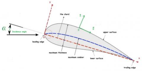
In this section, we present the asymptotic modeling of the two-dimensional laminar and stationary flow of a viscous incompressible fluid around wing airfoil with an incidence angle α (Figure1). The gravity force is neglected. The motion is governed by the Navier-Stokes and the continuity equations.
Figure 1. Diagram of the airfoil of the problem
It is convenient to choose the system of curvilinear coordinates (s, η). In figure (1), and are, respectively, the unit tangential and normal vectors.
The method of perturbation expansions is a well-established analytical tool that has found applications in many areas of fluid dynamics. A comprehensive survey of perturbation methods currently used in various engineering applications, when the problems are governed by partial differential equations [15-19].
The first step in a perturbation analysis is to identify the perturbation quantity. This is done by expressing the exact mathematical model in dimensionless form assessing the order of magnitude of different terms, and identifying the term that is small compared to others. At this level, we introduce scaled variables, namely:
$\left\{\begin{array}{c}\bar{s}=\frac{s}{c} ; \bar{\eta}=\frac{\eta}{c} ; \bar{p}=\frac{p}{\rho_{0} U_{0}^{2}} \\ \bar{u}=\frac{u}{U_{0}} ; \bar{w}=\frac{w}{U_{0}} ; \bar{\rho}=\frac{\rho}{\rho_{0}}=o(1) \equiv 1\end{array}\right.$ (1)
where, $u(s, \eta), w(s, \eta)$ and $p(s, \eta)$ are, respectively, the tangential and normal velocities and the pressure. For the scaling quantities are referenced by: c is the airfoil chord; $U_{o}$ and $\rho_{o}$ are, respectively, the velocity and the density in the obstacle upstream (no perturbed domain).
Using scaled variables, the non-dimensional equations of the problem, read as:
$\left\{\begin{array}{c}\bar{u}\left(\frac{\partial \bar{u}}{\partial \bar{s}}-\lambda \bar{w}\right)+(1-\lambda \bar{\eta}) \bar{w} \frac{\partial \bar{u}}{\partial \bar{\eta}}=-\frac{\partial \bar{p}}{\partial \bar{s}}+R_{e}^{-1}\left[\frac{1}{(1-\lambda \bar{\eta})}\left(\frac{\partial^{2} \bar{u}}{\partial \bar{s}^{2}}-\lambda \frac{\partial \bar{w}}{\partial \bar{s}}\right)-\lambda \frac{\partial \bar{u}}{\partial \bar{\eta}}\right. \left.-\frac{1}{(1-\lambda \bar{\eta})}\left(\lambda \frac{\partial \bar{w}}{\partial \bar{s}}+\lambda^{2} \bar{u}\right)+(1-\lambda \bar{\eta}) \frac{\partial^{2} \overline{\mathcal{U}}}{\partial \bar{\eta}^{2}}\right] \\ \bar{u}\left(\frac{\partial \bar{w}}{\partial \bar{s}}+\lambda \bar{u}\right)+(1-\lambda \bar{\eta}) \bar{w} \frac{\partial \bar{w}}{\partial \bar{\eta}}=-(1-\lambda \bar{\eta}) \frac{\partial \bar{p}}{\partial \bar{\eta}}+R_{e}^{-1}\left[\frac{1}{(1-\lambda \bar{\eta})}\left(\frac{\partial^{2} \bar{w}}{\partial \bar{s}^{2}}+\lambda \frac{\partial \bar{u}}{\partial \bar{s}}\right)\right.\left.-\lambda \frac{\partial \bar{w}}{\partial \bar{\eta}}+\frac{1}{(1-\lambda \bar{\eta})}\left(\lambda \frac{\partial \bar{u}}{\partial \bar{s}}-\lambda^{2} \bar{w}\right)+(1-\lambda \bar{\eta}) \frac{\partial^{2} \overline{\mathcal{W}}}{\partial \bar{\eta}^{2}}\right] \\ \left(\frac{\partial \bar{u}}{\partial \bar{s}}-\lambda \bar{w}\right)+(1-\lambda \bar{\eta}) \frac{\partial \bar{w}}{\partial \bar{\eta}}=0\end{array}\right.$ (2)
The numbers figuring in (2) are the Reynolds number $R_{e}=\frac{U_{o} c}{v}$ and the parameter $\lambda=\frac{c}{R}$ is the dimensionless surface curvature of this body. Here is considered the case where $\lambda=O(1)$.
Perturbation theory is based on the concept of an asymptotic solution. If the basic fluid dynamic equations that describe a precise flow problem can be expressed so that one of the parameters or variables is small (or very large). Indeed, the fluid considered is the "Air". It has low viscosity, and we can consider the limit of Reynolds number, $R_{e}^{-1} \rightarrow 0$, which is the singular case of vanishing viscosity.
Considering the limiting process, as:
$R_{e}^{-1} \rightarrow 0, \bar{s}$ and $\bar{\eta}$ are fixed of the order of 0(1) (3)
Obviously, if we simply delete the frictional (dissipative) terms proportional to Re on the right-hand side of Navier equation (2), then we obtain the Euler nonviscous incompressible system, namely:
$\left\{\begin{array}{l}\bar{u}\left(\frac{\partial \bar{u}}{\partial \bar{s}}-\lambda \bar{w}\right)+(1-\lambda \bar{\eta}) \bar{w} \frac{\partial \bar{u}}{\partial \bar{\eta}}=-\frac{\partial \bar{p}}{\partial \bar{s}} \\ \bar{u}\left(\frac{\partial \bar{w}}{\partial \bar{s}}+\lambda \bar{u}\right)+(1-\lambda \bar{\eta}) \bar{w} \frac{\partial \bar{w}}{\partial \bar{\eta}}=-(1-\lambda \bar{\eta}) \frac{\partial \bar{p}}{\partial \bar{\eta}} \\ \left(\frac{\partial \bar{u}}{\partial \bar{s}}-\lambda \bar{w}\right)+(1-\lambda \bar{\eta}) \frac{\partial \bar{w}}{\partial \bar{\eta}}=0\end{array}\right.$ (4)
The associated boundary conditions are:
$\bar{u}(\bar{s}, \bar{\eta}) \rightarrow \cos (\alpha)$ and $\bar{p}(\bar{s}, \bar{\eta}) \rightarrow 1$ when $\bar{\eta} \rightarrow+\infty$ (5)
The system (4) is so-called “outer” or “main no viscous” flow, obtained with the help of the Euler equations of motion. But in this case, unfortunately, because the order of the partial differential equation is reduced, the no-slip boundary condition disappears because the system (4) is not valid near the wall.
The singular perturbation is termed parameter perturbation or coordinates perturbation. So, the expansion fails in certain regions of the space-time domain. Thus, we find two limiting process, such as:
$R_{e}^{-1} \rightarrow 0$ and $\bar{\eta} \rightarrow 0$ when $\bar{S}$ fixed of the order of 0(1) (6)
And,
$R_{e}^{-1} \rightarrow 0 ; \bar{s} \rightarrow 0$ and $\bar{\eta} \rightarrow 0$ (7)
In this study, the relationships (6) and (7) show the existence of the singular regions [20], respectively, in the vicinity of the wall of the airfoil (boundary layer) and at the leading edge.
Indeed, during the limiting process (6), we find an indetermination related in particular to partial derivatives of second order relating to the effects of viscosity in our model, so we must consider the limiting process, called ‘’local’’, as:
$R_{e}^{-1} \rightarrow 0 ; \hat{\eta}=\frac{\bar{\eta}}{\delta_{1}\left(R_{e}^{-1}\right)}=\mathrm{O}(1) ; \bar{s}=\mathrm{O}(1) ; \hat{w}=\frac{\bar{w}}{\delta_{2}\left(R_{e}^{-1}\right)}$ (8)
where, $\delta_{i}\left(R_{e}^{-1}\right)$ (i=1,2) are the ‘gauge functions’ and determined according the “Least Degeneration Principle” (It consists to keep the maximum terms in system (2)). The gauge functions are defined as:
$\delta_{1}=\delta_{2}=R_{e}^{-1 / 2}$ (9)
The relation (9) characterizes the thickness of the two-dimensional boundary layer. Thus, taking into account (9) and substituting (8) into (2), we obtain, at the order 0 in $R_{e}^{-1 / 2}$, the “inner” or the “local-boundary layer” system, namely:
$\left\{\begin{array}{l}\hat{u} \frac{\partial u}{\partial \bar{s}}+\hat{w} \frac{\partial u}{\partial \eta}=-\frac{\partial \hat{p}}{\partial \bar{s}}+\frac{\partial^{2} u}{\partial \eta^{2}} \\ \frac{\partial \hat{p}}{\partial \hat{\eta}}=0 \\ \frac{\partial \hat{u}}{\partial \bar{s}}+\frac{\partial \hat{\omega}}{\partial \hat{\eta}}=0\end{array}\right.$ (10)
The associated boundary condition (no-slip condition) is:
$\hat{\eta}=0, \hat{u}(\bar{s}, \hat{\eta})=0, \hat{w}(\bar{s}, \hat{\eta})=0$ (11)
where: $\widehat{u}(\bar{s}, \hat{\eta}), \widehat{W}(\bar{s}, \hat{\eta})$ and $\hat{p}(\bar{s}, \hat{\eta})$ are, respectively, the velocity components and pressure in the boundary layer. The problem (10) is similar to the classical Prandtl problem of two-dimensional boundary layer on a plate flat. Also, we have $\frac{\partial \hat{p}}{\partial \widehat{\eta}}=0$, that means that the pressure gradient is substantially longitudinal and its value can be derived from the Bernoulli’s theorem valid outside the boundary layer (inviscid flow).
The leading edge is also a second singularity for the flow. The limiting process (8) generates an indetermination always related to the viscosity terms in our model. Let the variables and unknowns to distort such as:
$\left\{\begin{array}{l}\tilde{s}=\frac{\bar{s}}{\delta_{1}^{*}\left(R_{e}^{-1}\right)} ; \tilde{\eta}=\frac{\bar{\eta}}{\delta_{2}^{*}\left(R_{e}^{-1}\right)} \\ \tilde{u}=\frac{\bar{u}}{\delta_{3}^{*}\left(R_{e}^{-1}\right)} ; \tilde{w}=\frac{\bar{w}}{\delta_{4}^{*}\left(R_{e}^{-1}\right)} ; \tilde{p}=\frac{\bar{p}}{\delta_{5}^{*}\left(R_{e}^{-1}\right)}\end{array}\right.$ (12)
where, $\delta_{j}^{*}\left(R_{e}^{-1}\right)$ (j=1,…,5) are the ‘gauge functions’ and determined according the “Least Degeneration Principle”. Then, we find:
$\delta_{1}^{*}=\delta_{2}^{*}=\delta_{3}^{*}=\delta_{4}^{*}=\delta_{5}^{*}=R_{e}^{-1}$ (13)
Thus, taking into account (13) and substituting (12) into (2), we obtain, at the order 0 in $R_{e}^{-1}$, the “leading edge -boundary layer” system, namely:
$\left\{\begin{array}{l}\frac{\partial \tilde{p}}{\partial \tilde{s}}=\frac{\partial^{2} \tilde{u}}{\partial \tilde{s}^{2}}+\frac{\partial^{2} \tilde{u}}{\partial \eta^{2}} \\ \frac{\partial \tilde{p}}{\partial \tilde{\eta}}=\frac{\partial^{2} \tilde{w}}{\partial \tilde{s}^{2}}+\frac{\partial^{2} \tilde{w}}{\partial \tilde{\eta}^{2}} \\ \frac{\partial \tilde{u}}{\partial \tilde{s}}+\frac{\partial \tilde{w}}{\partial \tilde{\eta}}=0\end{array}\right.$ (14)
The associated boundary condition is:
$\tilde{u}(\tilde{s}=0, \tilde{\eta}=0)=0, \tilde{w}(\tilde{s}=0, \tilde{\eta}=0)=0$ (15)
The relation (15) also characterizes the stopping-point.
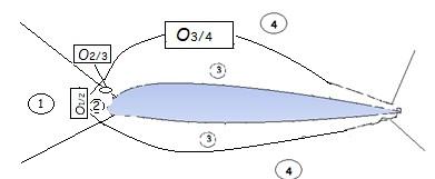
The asymptotic structure of our problem is illustrated in Figure (2).
Figure 2. Asymptotic structure around an airfoil
It includes four regions around the profile. There is also a small circular core in which, just as in the corresponding vicinity of the leading edge (2), the equations (14) and the boundary condition (15) apply. This region is matched upstream with the far field undisturbed (1), and downstream with the boundary layer (3) where the equations (10) and the boundary condition (11) apply. It is associated upward with the outer inviscid flow (4), the equations (4) and the boundary conditions (5) apply. The structure near the leading edge, contributes a correction to the boundary layer solution in region (3). So, we are interested in solving the boundary layer equations of our model.
Indeed, the “local-boundary layer” (in region (3)) and “main nonviscous” (in region (4)) flows should be matched onto the another so that both flows are valid in an overlap region ($O_{3 / 4}$ in Figure 2). In this overlap region, we have:
$\bar{u}(\bar{s}, \bar{\eta}) \cong \hat{u}(\bar{s}, \hat{\eta}) \cong \bar{U}_{e}(\bar{s})$
$\bar{\eta} \rightarrow 0 \quad \hat{\eta} \rightarrow \infty$ (16)
Via this matching, we can look for a solution of the form:
$\frac{\hat{u}(\bar{s}, \xi)}{\bar{U}_{e}(\bar{s})}=F(\xi) ; \xi=\frac{\hat{\eta}}{g(\bar{s})}$ (17)
where: $g(\bar{s})$ is a proportional function to the boundary layer thickness of the along the airfoil. Thus, $F(\xi)$ characterizes the evolution of the boundary layer thickness at any point of area (3). $\bar{U}_{e}(\bar{s})$ is the flow velocity outside the boundary layer (region (4)). The relation (17) characterizes a consistent, rational approximation of the real NSF (Navier-Stokes-Fourier Equations) slightly viscous fluid flows, called " affinity hypothesis".
Taking into account the relationship (17) and after a few operations in the system of equations (10), the transverse velocity is obtained as:
$\left.\hat{w}=\bar{U}_{e}(\bar{s}) g^{\prime}(\bar{s}) \xi H^{\prime}(\xi)-\bar{U}_{e}(\bar{s}) g^{\prime}(\bar{s})+\bar{U}_{e}^{\prime} g(\bar{s})\right] H(\xi)$ (18)
where:
$F(\xi)=H^{\prime}(\xi)$ (19)
(') denotes the derivative with respect to a variable.
We substitute (17) and (18) in the system (10), we obtain the following differential equation:
$\mathrm{H}^{\prime \prime\prime \prime}(\xi)+\mathrm{b}(1+\mathrm{a}) \cdot \mathrm{H}(\xi) \mathrm{H}^{\prime \prime \prime}(\xi)+\mathrm{b}(1-\mathrm{a}) \cdot \mathrm{H}^{\prime}(\xi) \mathrm{H}^{\prime \prime}(\xi)=0$ (20)
where:
$a=\frac{\bar{U}_{e}^{\prime}(\bar{s}) g(\bar{s})}{\bar{U}_{e}(\bar{s}) g^{\prime}(\bar{s})}=c s t$
$b=\bar{U}_{e}(\bar{s}) g(\bar{s}) g^{\prime}(\bar{s})=c s t$ (21)
whose solving (20) is purely numerical.
We note in our problem that the transverse velocity is negligible compared to the longitudinal velocity. Thus, $\hat{w}$ is of the order $R_{e}^{-1 / 2}$, and consequently, at the order 0 in $R_{e}^{-1 / 2}$, we assume:
$\hat{\mathcal{W}} \cong 0$ (22)
So, approximately from (18), we obtain the following linear differential equation:
$\xi H^{\prime}(\xi)-(1+a) H(\xi) \cong 0$ (23)
whose the solution is:
$H(\xi)=A \xi^{l+a} ; H^{\prime}(l) \cong O(1)$ (24)
The solution (24) is substituted into (20), so, we find that it is validated at the order of $r_{e}^{-1}$. We remark that this solution is a good approximation if:
m=-1; m=0; m=1/3; m=1/2 (25)
where: $m=\frac{a}{a+2} ; m \neq 1$.
The relations (21) allow determining the function $g(\bar{s})$ and the velocity $\overline{U_{e}}(\bar{s})$, as:
$g(\bar{s})=\left(\frac{2 b}{(1-m) \cdot C} \bar{s}+B\right)^{\frac{1-m}{2}}$ (26)
$\bar{U}_{e}(\bar{s})=C .\left(\frac{2 b}{(1-m) \cdot C} \bar{s}+B\right)^{m}$ (27)
where: $m=\frac{a}{a+2} ; m \neq 1$; C is a constant.
We note that $g(\bar{s})$ characterize the boundary layer thickness, and when $\bar{S} \cong R_{e}^{-1}$ the function $g(\bar{s})$ is at the order $O\left(R_{e}^{-1}\right)$. At the limit, when $R_{e}^{-1} \rightarrow 0$ then $g(\bar{s}) \rightarrow 0$, we can deduce from the relation (26):
$B \cong 0$ (28)
Finally, taking into account the relations (17), (19), (24), (26) and (27), we deduce the velocity field in the ‘’local boundary layer’’:
$\hat{u}(\eta)=A \cdot C \cdot\left(\frac{1+m}{1-m}\right) \cdot \eta^{\frac{2 m}{1-m}}$ (29)
The relationship (29) satisfies the non-slip condition if: 0 ˂m˂1.
The pressure can be derived from the Bernoulli’s theorem $\left[\frac{d \hat{p}(\bar{s})}{d \bar{s}}=-\frac{1}{2} \frac{d}{d s} \bar{U}_{e}^{2}(\bar{s})\right]$ valid outside the boundary layer (inviscid flow), namely:
$\hat{p}(\bar{s})=-\frac{1}{2} \cdot C^{2(1-m)} \cdot\left(\frac{2 b}{(1-m)}\right)^{2 m} \cdot(\bar{s})^{2 m}+D_{3}$ (30)
We note that despite the conditions (5), (11) and (24), the constants A, b, C and D3 remain undetermined. These constants will be determined by the matching conditions between regions illustrated in figure (2). For this, we must solve the problem in the vicinity of the leading edge.
Indeed, after a few operations in the system of equations (14), the longitudinal velocity satisfies the differential equation:
$\frac{\partial^{4} \tilde{u}(\tilde{s}, \tilde{\eta})}{\partial \tilde{s}^{4}}+2 \frac{\partial^{4} \tilde{u}(\tilde{s}, \tilde{\eta})}{\partial \tilde{\eta}^{2} \partial \tilde{s}^{2}}+\frac{\partial^{4} \tilde{u}(\tilde{s}, \tilde{\eta})}{\partial \tilde{\eta}^{4}}=0$ (31)
Using the method of separating variables, we obtain the following approximate solution:
$\tilde{u}(\tilde{s}, \tilde{\eta})=C_{1} \cdot \cos (\beta \cdot \tilde{s})\left(1-e^{-\beta \cdot \tilde{\eta}}\right)$ (32)
Therefore, we deduce the following results:
$\tilde{w} \cong 0 \quad ; \tilde{p}(\tilde{s})=-C_{1} \cdot \beta \cdot \sin (\beta \cdot \tilde{s})+D_{2}$ (33)
Now, we will try to estimate the constants A, b, C, C1, D2, D3 and m. Indeed, we consider, first, the interface connecting the upstream infinity (1) and the leading edge region (2), denoted O1/2. In this overlap region, we have:
$O_{1 / 2}=\{\tilde{s} \cong O(1) ; \quad \tilde{\eta} \rightarrow+\infty\}$ (34)
And also:
$\left.\tilde{u}(\tilde{s}, \tilde{\eta})\right|_{O_{1 / 2}}=\cos (\alpha) ;\left.\tilde{p}(\tilde{s})\right|_{O_{1 / 2}}=1$ (35)
Finally, taking into account the relation (35), we find ($\cos (\beta) \neq 0$):
$C_{1}=\frac{\cos (\alpha)}{\cos (\beta)} ; D_{2}=1+\beta \cos (\alpha) \operatorname{tg}(\beta)$ (36)
Then, in the overlap zone, denoted O2/3, between regions (2) and (3), we have:
$O_{2 / 3}=\left\{\tilde{s}=\tilde{\eta} \cong O(1) ; \bar{s} \cong R_{e}^{-1}, \hat{\eta} \cong R_{e}^{-1 / 2}\right\}$ (37)
Also:
$\left.\left.\tilde{u}(\tilde{s}, \tilde{\eta})\right|_{O_{2 / 3}} \equiv \hat{u}(\hat{\eta})\right|_{O_{2 / 3}}$
$\left.\left.\tilde{p}(\tilde{s})\right|_{O_{2 / 3}} \equiv \hat{p}(\bar{s})\right|_{O_{2 / 3}}$ (38)
Taking into account the first relation of (38), we find:
$\cos (\alpha)\left(1-e^{-\beta}\right) \cong A C\left(\frac{1+m}{1-m}\right)\left(R_{e}^{-1}\right) \frac{m}{1-m}$ (39)
For the relation (39) to be significant, it is necessary that $\beta$ be very small $\left(1-e^{-\beta} \cong \beta, \cos (\beta) \cong 1\right)$. So, in this case, (39) is satisfied if:
$\beta \equiv R_{e}^{-1} \quad$ and $\quad m=\frac{1}{2}$ (40)
Hence, we can deduce:
$C=\left(\frac{1-m}{1+m}\right) \cdot \frac{\cos (\alpha)}{A} ; A \neq 0 ; D_{2} \cong 1$ (41)
Finally, at the limit when $R_{e}^{-1} \rightarrow 0$, the second relation of (38) gives:
$D_{3} \cong 1$ (42)
The “leading edge” and the ‘’local boundary layer’’ solutions together are used to construct the uniformly valid solution around the airfoil as a composite asymptotic expansion
$\Psi(\bar{s}, \bar{\eta})=\tilde{\Psi}(\bar{s}, \bar{\eta})+\hat{\Psi}(\bar{s}, \bar{\eta})-($ common development between the two solutions)
$u(\bar{s}, \eta)=\cos (\alpha) \cdot \cos (\bar{s})\left(1-e^{-R_{e}^{-1 / 2}} \cdot \hat{\eta}\right)+\cos (\alpha) \cdot \eta^{2}-R_{e}^{-1} \cdot \cos (\alpha)$ (43)
$w(\bar{s}, \hat{\eta}) \cong 0$ (44)
$p(\bar{s})=-R_{e}^{-1} \cdot \cos (\alpha) \cdot \sin (\bar{s})-\frac{2 b}{3 A} \cdot \cos (\alpha) \cdot \bar{s}+1$ (45)
The solutions (43), (44) and (45) depend on several parameters as angle of attack and Reynolds number. But, we note, at this level, that the constants A and b are still undetermined. Then, empirical expressions must be derived for these constants. The basic assumption for this derivation is that the flow on one side of the airfoil is completely separated so that the airfoil can be approached by a curved plate.
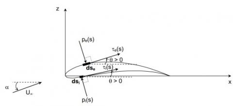
The aerodynamic forces, lift and drag, applied to an airfoil induce a surface pressure distribution $p(\bar{s})$ and a surface distribution of friction by viscous shear stress $\tau(\bar{s})$ on the lower surface (subscript i) and the upper surface (subscript e) of the profile.
Figure 3. Pressure distribution and viscous friction on the airfoil
where $\theta$ is the angle between the unit tangential vector ($\vec{e}$) and x-axis.
At any point in the flow where the local pressure is $p(\bar{s})$ the Pressure Coefficient $C_{p}=\left(C_{p}=\frac{p^{*}-p_{\infty}}{p_{\infty}}\right)$ is defined, for our model, as:
$C_{p}=p(\bar{s})-1=-R_{e}^{-1} \cdot \cos (\alpha) \cdot \sin (\bar{s})-\frac{2 b}{3 A} \cdot \cos (\alpha) \bar{s}$ (46)
And the coefficient of friction $C_{f}\left(C_{f}=\frac{2 \tau}{\rho U_{\infty}^{2}} \text { with } \tau=\left.\mu \frac{\partial u}{\partial \eta}\right|_{\eta=0}\right)$ is defined, for our model, as:
$C_{f}=\left.2 \cdot R_{e}^{-1} \cdot \frac{\partial u}{\partial \hat{\eta}}\right|_{\hat{\eta}=0}=2 \cdot R_{e}^{-3 / 2} \cdot \cos (\alpha) \cdot \cos (\bar{s})$ (47)
Once the numerical values for Cp and Cfhave been computed they may be used to calculate the lift and drag coefficients CLand CDusing the following relationships, namely:
$C_{L}=C_{n} \cos (\alpha)-C_{a} \sin (\alpha)$
$C_{D}=C_{n} \sin (\alpha)+C_{a} \cos (\alpha)$ (48)
where, Cn and Ca are, respectively, the normal and parallel forces (to the chord) coefficients. Considering the following change of variables, namely:
$d \bar{s}_{e / i} \cos (\theta)=d \bar{x}_{e / i}$
$d \bar{s}_{e / i} \sin (\theta)=d \bar{z}_{e / i}$ (49)
Then, these coefficients become:
$C_{n}=\int_{0}^{1}\left(-C_{p, e} \cdot f_{e}(\bar{s})+C_{f, e} \cdot g_{e}(\bar{s})\right) d s_{e}+\int_{0}^{1}\left(C_{p, i} \cdot f_{i}(\bar{s})+C_{f, i} \cdot g_{i}(\bar{s})\right) d s_{i}=C_{n, e}+C_{n, i}$
$C_{a}=\int_{0}^{1}\left(C_{p, e} \cdot g_{e}(\bar{s})+C_{f, e} \cdot f_{e}(\bar{s})\right) d s_{e}+\int_{0}^{1}\left(-C_{f, i} \cdot g_{i}(\bar{s})+C_{f, i} \cdot f_{i}(\bar{s})\right) d s_{i}=C_{a, e}+C_{a, i}$ (50)
where: $f_{e / i}$ and $g_{e / i}$ are the functions which depend only of the curvilinear coordinates of the airfoil, such as:
$f_{e / i}=\frac{d \bar{x}_{e / i}}{d \bar{s}_{e / i}} ; \quad g_{e / i}=\frac{d \bar{z}_{e / i}}{d \bar{s}_{e / i}}$ (51)
where, ($\overline{x_{e / l}}=\frac{x_{e / i}}{c}, \overline{z_{e / l}}=\frac{z_{e / i}}{c}$) represent the coordinates of the NACA airfoil.
The approximate solution of the "boundary layer", around the NACA airfoil and outside the region near the nose of the leading edge, is valid for b constant (21). Thus, the aerodynamic coefficients of lift and drag (46) and (48) depend on the constants b and A.
Several writers on the flow around airfoils show that the angle of attack, when it increases, greatly influences the aerodynamic characteristics of the aircraft.
Therefore, several approximate methods have been invested for the aerodynamic coefficients for a wide range of incident angle [21]. Indeed, we suppose that the constant A is strongly influenced by the incidence angle $\alpha$: A(a) and satisfies a trigonometric empirical relation, such that:
$A(\alpha)=A_{\alpha}=\cos \left(\alpha+n_{\alpha} \theta\right)$ (52)
where: $n_{a}$ is an adjustment factor that depends on $\alpha$ and $\theta$ characterizes the deflection of the boundary layer thickness. Since b is related to A( $\alpha$), then we assume:
$b=b(\alpha)=\beta_{\alpha} \cos \left(\alpha+n_{\alpha} \theta\right)$ (53)
$\beta_{a}$ is a proportionality constant with A( $\alpha$).
We know that b is a constant, and consequently $n_{a}$ and $\theta$ will be determined in such a way that all curves converge at one single point (b, $\theta$). This method requires at least three experimental or simulation data.
Firstly, to determine the functions $f_{e / i}$ and $g_{e / i}$, we proceed by the method of Lagrange interpolation in the Maple software ‘’ CurveFitting [Interactive]’’ module.
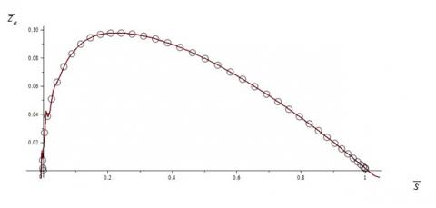
Plotting the data of the upper surface for NACA 43013, the software gives the profile like below:
Figure 4. Upper surface profile of NACA 43013
From Figure (4), we find discontinuities in the profile curve. Thus, for a great precision, we subdivide the range of $\bar{S}$ in three pieces, as:
$\bar{x}_{e}(\bar{s})=-0.017+0.92 \bar{s}+0.27 \bar{s}^{2}-0.18 \bar{s}^{3}$ (54)
$\left\{\begin{array}{ll}\overline{\mathrm{z}}_{\mathrm{e} 1}(\overline{\mathrm{s}})=-0.0011+0.9 \overline{\mathrm{s}}+3.6 \overline{\mathrm{s}}^{2}-111.5 \overline{\mathrm{s}}^{3} & \overline{\mathrm{s}} \in[0,0.04] \\ \overline{\mathrm{z}}_{\mathrm{e} 2}(\overline{\mathrm{s}})=0.0012+1.1 \overline{\mathrm{s}}-4.1 \overline{\mathrm{s}}^{2}+4.9 \overline{\mathrm{s}}^{3} & \overline{\mathrm{s}} \in[0.04,0.2] \\ \overline{\mathrm{z}}_{\mathrm{e} 3}(\overline{\mathrm{s}})=0.09+0.1 \overline{\mathrm{s}}-0.3 \overline{\mathrm{s}}^{2}+0.8 \overline{\mathrm{s}}^{3} & \overline{\mathrm{s}} \in[0.22,1]\end{array}\right.$ (55)
By the same procedure as above, for the lower surface of NACA airfoil, we find:
$\bar{x}_{i}(\bar{s})=0.002+1 \bar{s}-0.01 \bar{s}^{2}+0.006 \bar{s}^{3}$ (56)
$\left\{\begin{array}{ll}\bar{z}_{i 1}(\bar{s})=-0.9 \bar{s}+22.6 \bar{s}^{2}-217 \bar{s}^{3} & \overline{\mathrm{s}} \in[0,0.04] \\ \bar{z}_{i 2}(\bar{s})=-0.01+0.07 \bar{s}-1.05 \bar{s}^{2}+1.8 \bar{s}^{3} & \overline{\mathrm{s}} \in[0.04,0.18] \\ \bar{z}_{i 3}(\bar{s})=-0.004-0.16 \bar{s}+0.24 \bar{s}^{2}-0.07 \bar{s}^{3} & \overline{\mathrm{s}} \in[0.18,1]\end{array}\right.$ (57)
The relations below show that the functions obtained from our model accurately represent the profile, compared to the actual NACA profile; we obtain an average relative error of 3%.
Substituting the relations (54), (55), (56) and (57) in the relations (50), taking into account (51), to determine the aerodynamic coefficients of NACA wing profile.
Now, with Ansys fluent, we can simulate the flow around the airfoil NACA, in order to validate our model and to produce a satisfactory approximation of airfoil aerodynamic coefficients in the whole α range with the lowest possible number of data points necessary to tune the model.
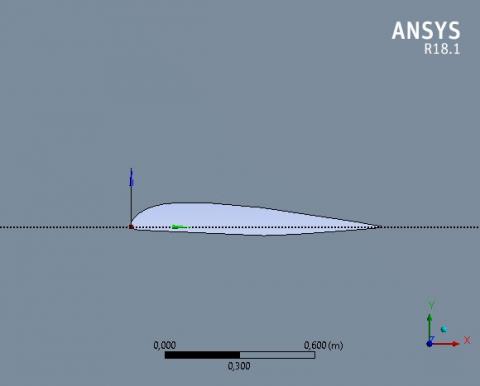
Indeed, for CFD simulation the coordinates for NACA 43013 of the airfoil is imported from CATIA V5 and the geometry is created that will use for the simulation as in Figure (5).
Figure 5. Geometry of NACA 43013 airfoil
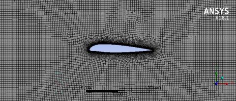
Figure 6. Mesh generation for NACA 43013
In order to analyze fluid flows, flow domains are split into smaller subdomains [22]. Subdomains are made up of geometric primitives like quadrilaterals in 2D [23]. Mesh analysis is performed by assigning the value 5 for relevance and size function is proximity and curvature. Also, by assuming relevance center is fine and smoothing is high.
Typically, the best way to capture effects in the boundary layer is by accommodating higher number of cells in the direction normal to the fluid flow.
We will need to choose element types that can be stacked one over the other. In Ansys fluent, we have achieving 271495 nodes and 270061 elements stacking in the direction normal to the boundary using a feature called “inflation layer”. Essentially, we can inflate the mesh with 12 layers from the surface of the boundary (2 edges) until we cover the boundary layer thickness fully. Finally, the automatic method has been applied for the mesh (Figure 6).
For laminar, steady and incompressible flow and viscous fluid, we consider a Reynolds number Re =3.42 105 and with a free upstream velocity of 5 m/s. The fluid (air), at room temperature 288.16 K°, has a density 1.225 kg/m3 and a dynamic viscosity 1.789. 105 kg/m.s. We will also define the gauge pressure at the inlet to be zero. As for the airfoil itself, we will treat it like a wall. No slip boundary conditions are imposed. For causing the flow to remain straight up (top) and down (bottom), it will impose a condition “slip wall”, that is to say a wall without friction.
To validate our model, we made a comparative study between simulation and model for drag and lift coefficients as shown in the following tables and graphs:
Table 1. Results of the drag coefficient of the simulation and our model, for 0°˂ α ˂ 20 °.
|
Incidence ° |
simulation |
Model_3points (0,2,4) |
Model_3points (0,8,10) |
Model_4points(0,8,10,20) |
|
0 |
9.83E-03 |
9.81E-03 |
9.87E-03 |
9.87E-03 |
|
2 |
1.94E-02 |
1.93E-02 |
2.01E-02 |
1.86E-02 |
|
4 |
2.89E-02 |
2.88E-02 |
2.96E-02 |
2.73E-02 |
|
6 |
4.38E-02 |
3.79E-02 |
3.90E-02 |
3.60E-02 |
|
8 |
6.09E-02 |
4.69E-02 |
6.11E-02 |
6.11E-02 |
|
10 |
4.98E-02 |
5.31E-02 |
5.00E-02 |
5.01E-02 |
|
15 |
6.13E-02 |
7.29E-02 |
6.87E-02 |
5.88E-02 |
|
20 |
7.28E-02 |
9.06E-02 |
8.54E-02 |
7.31E-02 |
Table 1 shows the results of the drag coefficient obtained by our model in the case of the nonlinear empirical relationship (52 & 53). These require 3 or 4 data simulation Ansys fluent to determine the constants b and A.
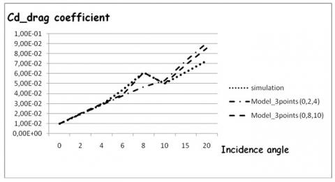
The Figure 7.(1) represents the intersection of the curves b0°, b2° and b4° at a single point (b=0,184;ϴ=18,436°) and as a result, it is determined: A0°=0,98682; A2°=0,9371; A4°=0,9243 and calculates Ameans=0,9432, which allows to determine with a good approximation, the drag coefficients. Similarly, Figure 7. (2) represents the intersection of the curves b0°, b8° and b10° at a single point (b=0,092; ϴ=61,23°). The Figure 7.(3) represents the intersection of the curves b0°, b8°, b10° and b20° at a single point (b=0,092 ; ϴ=61,23°). The same procedure is used as previously to determine the drag coefficients.
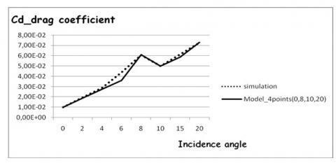
The simulation curve of the drag coefficient has two remarkable points (2 peaks) for angles of incidence 8 ° and 10 °. The Figures 8a and 8b show that the model, according to the approach mentioned above, is a good approximation when we take into account these remarkable data of the simulation.
Thus, we note that this approach method for 4 data points of the simulation is an excellent approximation of the drag coefficient with an error of 0.78%.
Table 2 shows the results of the lift coefficient obtained by our model in the case of the 2nd approach. The process of determining the constants A and b is the same as previously.
Figure 7. Determination of the constant b of the drag coefficient uniquely
Figure 8a. Comparison of the drag coefficient of the simulation and our model
Figure 8b. Comparison of the drag coefficient of the simulation and our model
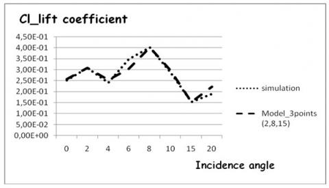
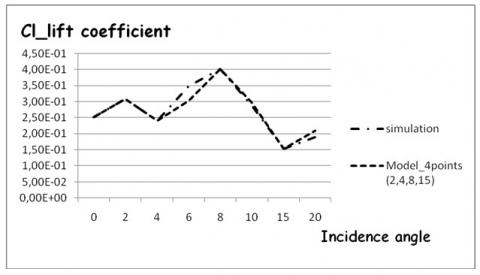
Table 2. Results of the lift coefficient of the simulation and our model, for 0°˂ α ˂ 20 °
|
Incidence ° |
simulation |
Model_3points (2,8,15) |
Model_4points (2,4,8,15) |
|
0 |
2.52E-01 |
2.56E-01 |
2.53E-01 |
|
2 |
3.08E-01 |
3.07E-01 |
3.08E-01 |
|
4 |
2.40E-01 |
2.54E-01 |
2.40E-01 |
|
6 |
3.50E-01 |
3.04E-01 |
3.04E-01 |
|
8 |
4.02E-01 |
4.01E-01 |
4.02E-01 |
|
10 |
2.89E-01 |
2.97E-01 |
2.97E-01 |
|
15 |
1.53E-01 |
1.53E-01 |
1.53E-01 |
|
20 |
1.90E-01 |
2.23E-01 |
2.11E-01 |
Figure 9. Determination of the constant b of the lift coefficient uniquely
Figures 9 (1 & 2) show, respectively, the intersection of the curves b2°, b8° and b15° at a single point (b= 0,18 ;ϴ=64,933°) and the intersection of curves b2°, b4°, b8° et b15° at a single point (b= 0,18 ;ϴ=64,96°). This allows determining with great accuracy the lift coefficients.
The simulation curve of the lift coefficient has four remarkable points (4 peaks) for angles of incidence 2 °, 4 °, 8 °and 15 °.
Figure 10a. Comparison of the lift coefficient of the simulation and our model
Figure 10b. Comparison of the lift coefficient of the simulation and our model
As before, the Figures 10a and 10b show that the model, according to the second approach, is a good approximation when we take into account these remarkable data of the simulation. Thus, we note that the 2nd approach method for 4 data points of the simulation is an excellent approximation of the lift coefficient with an error of 5%.
The results obtained in the present paper globally show the importance of the low viscosity effect in the modeling of the behaviors and response characteristics of a tow-dimensional laminar boundary layer around an airfoil and the power asymptotic approach for this modeling.
The several characteristics usually encountered in the fluid-structure interaction are correctly predicted by our model.
In case of empirical approximation, four points obtained using 2D CFD are sufficient to tune our model. The method produced satisfactory results for the Cl and Cd curves in the whole α range: 0°≤ α ≤ 20 °. We have numerically modeled by Ansys following the interaction between the flow and a NACA43013 profile having a different incidence angles, and Reynolds number Re =3,42 105. When this model is applied to study the boundary layer over solid surfaces, the matching of predictions and numerical simulations with our model remains quantatively acceptable. Moreover, they allow confirming much experimental behavior.
[1] Brückern, C., Weidner, C. (2014). Influence of self-adaptive hairy flaps on the stall delay of an airfoil in ramp-up motion. Journal of Fluids and Structures, 47: 31-40. http://doi.org/10.1016/j.jfluidstructs.2014.02.014
[2] Sellers, W.L.I., Singer, B.A., Leavitt, L.D. (2003). Aerodynamics for revolutionary air vehicles. AIAA (American Institute of Aeronautics and Astronautics), pp. 2004-3785. http://doi.org/10.2514/6.2003-3785
[3] Gença, M.S., Karasu, I., Hakan Açıkel, H. (2012). An experimental study on aerodynamics of NACA2415 aerofoil at low Re numbers. Experimental Thermal and Fluid Science, 39: 252-264. http://doi.org/10.1016/j.expthermflusci.2012.01.029
[4] Strickland, J.H., Webster, B.T., Nguyen, T. (1979). A vortex model of the Darrieus turbine: An analytical and experimental study. Fluids Eng, 101(4): 500-505. http://doi.org/10.1115/1.3449018
[5] Cardona, J.L. (1984). Flow curvature and dynamic stall simulated with an aerodynamic free-vortex model for VAWT. Wind Eng, 8: 135-143.
[6] Laneville, A., Vittecoq, P. (1986). Dynamic stall: the case of the vertical axis wind turbine. Sol. Energy Eng, 108(2): 140-145. http://doi.org/10.1115/1.3268081
[7] Vandenberghe, D., Dick, E. (1987). A free vortex simulation method for the straight bladed vertical axis wind turbine. Wind Eng. Ind. Aerodyn, 26(3): 307-324. http://doi.org/10.1016/0167-6105(87)90002-X
[8] Simão Ferreira, C.J., Van Zuijlen, A., Bijl, H., Van Bussel, G., Van Kuik, G. (2010). Simulating dynamic stall in a two-dimensional vertical-axis wind turbine: verification and validation with particle image velocimetry data. Wind Energy, 13(1): 1-17. http://doi.org/10.1002/we.330
[9] Castelli, M.R., Englaro, A., Benini, E. (2011). The Darrieus, wind turbine: proposal for a new performance prediction model based on CFD. Energy, 36(8): 4919-4934. http://doi.org/10.1016/j.energy.2011.05.036
[10] McLaren, K., Tullis, S., Ziada, S. (2012). Computational fluid dynamics simulation of the aerodynamics of a high solidity, small‐scale vertical axis wind turbine. Wind Energy, 15(3): 349-361. http://doi.org/10.1002/we.472
[11] Li, Q.A., Takao, M., Yasunari, K., Yuya, H., Nakai, A., Kasuya, T. (2017). Study on stall behavior of a straight-bladed vertical axis wind turbine with numerical and experimental investigations. Journal of Wind Engineering & Industrial Aerodynamics, 164: 1-12. http://doi.org/10.1016/j.jweia.2017.02.005
[12] Morshed, K.N. (2010). Experimental and numerical investigations on aerodynamic characteristics of savonius wind turbine with various overlap ratios. Master of Science in Applied Engineering, Georgia Southern University, Statesboro, Georgia 30458.
[13] Zhang, Y., Igarashi, Y., Hu, H. (2011). Experimental investigations on the performance degradation of a low-Reynolds-number airfoil with distributed leading-edge roughness. 4-7 January 2011. 49th AIAA Aerospace Sciences Meeting Including the New Horizons Forum and Aerospace Exposition, Orlando, Florida, AIAA-1102. http://doi.org/10.2514/6.2011-1102
[14] Yang, Z., Haan, F.L., Hui, H. (2007). An experimental investigation on the flow separation on a low-Reynolds-number airfoil. 45th AIAA Aerospace Sciences Meeting and Exhibit, Jan 8 - 11, 2007, Reno, Nevada AIAA-0275. http://doi.org/10.2514/6.2007-275
[15] Zeytounian, R.K. (2002). Asymptotic Modelling of Fluid Flow Phenomena. Fluid Mech, 471: 409-410.
[16] Hasnaoui, M., Agouzoul, M. (2002). Linear spectral analysis of three-dimensional inhomogeneous turbulent free jet under realistic atmospheric conditions. AMSE Journals, Modelling B, 71(5): 1-22.
[17] Hasnaoui, M. (2007). Influence of Coriolis Forces on The Dynamique of a Turbulent Jet. AMSE Journals, Modelling B, 76(6): 63-76.
[18] Slimani, A., Hasnaoui, M. (2007). The Gravity Waves in Atmospheric Shear Flows with Coriolis Forces. AMSE Journals, Modelling B, 76(4): 20-39.
[19] Mehdari, A., Hasnaoui, M., Agouzoul, M. (2018). Analytical Modelling for Newtonian Fluid Flow Through an Elastic Tube. Diagnostyka, 19(1): 2449-5220. http://doi.org/10.29354/diag/81237
[20] Caillerie, D., Cousteix, J., Mauss, J. (2016). Méthodes asymptotiques en mécanique. Edition Cépaduès, eBook ISBN: 978236493503, Ref:1503, Toulouse, France.
[21] Apostolyuk, V. (2007). Harmonic representation of aerodynamic lift and drag coefficients. AIAA Journal of Aircraft, 44(4): 1402-1404. http://doi.org/10.2514/1.30250
[22] Dinesh, K.G., Vignesh, K.R., Ajay, K.M., Srikanth, J.V.R., Soorya, P. (2013). Numerical investigation of vicous drag reduction using riblets. Adv. Aerosp. Sci. App, 3(2): 75-82.
[23] Cousin, H.S., Torres, R.F., Zabihian, F., Panta, Y. (2015). Design and analysis of fluid flows through PIV and CFD modeling. In Proceedings of the 2015 ASEE North Central Section Conference.