Hadji Chaabane | Khodja Djalal Eddine | Chakroune Salim* | Hadji Djamel
OPEN ACCESS
In this paper, Speed Sensorless Vector Control of Double star Induction machine DSIM using sliding mode observer is presented. The search for the gains of conventional Luenberger observer in the sense of stability Lyapunov, oriented to sliding mode observer form, but the sign function caused the chattering effect, the replace it by function smooth are adopted. As a result, application of DSIM speed sensorless vector control using sliding mode has shown that is robust to load disturbances and / or reference speed change. The proposed control scheme is verified by simulation.
double star induction machine DSIM, indirect vector control, sensorless, Luenberger, lyapunov stability, sliding mode observer
The majority of the controls rest completely on the assumption that all the state is known at every moment for technological reasons (material, industrialization, etc.) of stability (disrepair of the elements of measurement) or economic (cost of the sensors material) in many applications the measurement of all parameters is not possible. It is then necessary, using measurements available to reconstruct the not measured variables of state. It is major problem of the observation.
We find these problems in a context more general than that of the controls, such as for example the diagnosis, the detection of disrepair, security where the knowledge of the state of the system can be necessary. In addition: For the laws of the control as sophisticated, a main problem which is the necessitate use a mechanical sensor (speed, flux, ...). This imposes an over cost and increases the complexity of the industrial assembly. In some industrial fields such as operational security, therefore operation without a mechanical sensor makes it possible, on the one hand, to reduce costs (no sensor to implanted) and maintenance, and secondly to proposed a solution degraded, but functional to applications when disrepair faults.
From this point of vision, the primary objective of this article consists a determining the quantities (speed and flux) of the double star asynchronous machine DSIM by using only electric quantities measured.
These techniques, used to replace the information given by mechanical sensors, are sometimes called software sensors. In the same context, several observation approaches without mechanical sensor of the asynchronous double star machine are developed, in the literature, we can cite those based on artificial intelligence like neural networks [1, 2] and Bakcteebing [3].
Another approach from the automatic is based on a machine behavior model. We designed several categories: extended Kalman filters [4, 5] and nonlinear observers such as sliding modes [6, 7], and the observers with grand gain [8] and the extended Luenberger observer [9, 10] which difficult to guarantee the local convergence and stability [11, 12], whose main difficulties are stability, since we found that for these laws of controls without mechanical sensor, there was no demonstration of global convergence of the system ''Control + Observer" in closed loop.
However, this work is oriented in direction based stability Lyapunov improving the simple Luenberger observer by sliding mode control and minimizing the chattering effect. Moreover, the control law proposed guarantees largely stability and asked robustness. The work will be tested and evaluated in normal and severe machine operating conditions DSIM.
This paper is organized as following: the field oriented of dual star induction motor (DSIM) is described in section 2, section 3 reviews the estimation of the rotor speed and rotor flux by Luenberger observer, in section 4 sliding mode speed observer of DSIM developed is discussed (using only electrical measurements). Finally, simulations result and conclusion are given in sections 5.
2.1 Principle
The principle of vector control is to operate the asynchronous machine like the DC machine with separate excitation, by decoupling the torque control and the flux control. In fact, we propose to study the vector control of DSIM. The adopted control strategy consists in keeping the quadrature flux equals to zero $\left(\Phi_{q r}=0\right)$ and the direct flux equals to the reference $\left(\Phi_{d r}=\Phi_{r}^{*}\right)$ [9].
2.2 Application
The application of this control technique makes it possible to obtain speed and torque control performance comparable to DC machine.
Based on the main control strategy $\left(\Phi_{d r}=\Phi_{r}^{*}, \Phi_{q r}=0\right)$ it is possible to finalize the expression of the electromagnetic torque by:
${{T}_{e}}=P\frac{{{L}_{m}}}{{{L}_{m}}+{{L}_{r}}}\left( {{I}_{qs1}}+{{I}_{qs2}} \right){{\Phi }_{r}}$ (1)
Therefore, the main objective according to Chaabane et al. [13, 14] is to provide reference signals for the voltage inverter which supplies DSIM. Note X* for reference: the desired reference paths for (torque, flux, voltages and currents).
The control based on the orientation of the rotor flux gives better results with respect to the orientation of the stator flux [15, 16]. Indeed, the application of this orientation the equations system of the machine becomes.
With:
$\mu_{1}=\frac{P}{J} \frac{L_{m}}{L_{m}+L_{r}}, \quad \mu_{2}=\frac{R_{r}}{L_{m}+L_{r}}$ and $\omega_{s r}^{*}$ the slip angular frequency. $T_{r}=\frac{L_{r}}{R_{r}}$ denotes the rotor time constant.
$\omega_{s}^{*}=\omega_{s r}^{*}+\omega_{r}$ (2)
The sliding speed is given by:
$\omega _{sr}^{*}={{\mu }_{2}}{{L}_{m}}\left( I_{qs1}^{*}+I_{qs2}^{*} \right)$ (3)
From the direct vector control equations, we derive the following system of equations of states [5, 17, 18].
$\left\{ \begin{align} & {{{\dot{I}}}_{ds1}}=\frac{1}{{{L}_{s1}}}\left[ v_{ds1}^{*}-{{R}_{s1}}{{I}_{ds1}}+\omega _{s}^{*}\left( {{L}_{s1}}{{I}_{qs1}}+{{T}_{r}}\Phi _{r}^{{}}\omega _{sr}^{*} \right) \right] \\ & {{{\dot{I}}}_{qs1}}=\frac{1}{{{L}_{s1}}}\left[ v_{qs1}^{*}- {{R}_{s1}}{{I}_{qs1}}-\omega _{s}^{*}\left( {{L}_{s1}}{{I}_{ds1}}+\Phi _{r}^{*} \right) \right] \\ & {{{\dot{I}}}_{ds2}}=\frac{1}{{{L}_{s2}}}\left[ v_{ds2}^{*}- {{R}_{s2}}{{I}_{ds2}}+\omega _{s}^{*}\left( L{}_{s2}{{I}_{qs2}}+{{T}_{r}}{{\Phi }_{r}}\omega _{sr}^{*} \right) \right] \\ & {{{\dot{I}}}_{qs2}}=\frac{1}{{{L}_{s2}}}\left[ v_{qs2}^{*}-{{R}_{s2}}{{I}_{qs2}}-\omega _{s}^{*}\left( {{L}_{s2}}{{I}_{ds2}}+\Phi _{r}^{*} \right) \right] \\ \end{align} \right.$ (4)
$\left\{ \begin{align} & {{{\dot{\Phi }}}_{r}}={{\mu }_{2}}{{\Phi }_{r}}+{{\mu }_{2}}{{L}_{m}}\left( {{I}_{ds1}}+{{I}_{ds2}} \right) \\ & \dot{\omega }=\frac{1}{j}\left[ (\left[ \frac{{{L}_{m}}}{{{L}_{m}}+{{L}_{r}}}\left( {{I}_{qs1}}+{{I}_{qs2}} \right)\Phi _{r}^{*}-{{T}_{L}}-{{B}_{\omega }}\omega \right]) \right] \\ \end{align} \right.$ (5)
$R_{r}$: Rotor resistance;
$R_{s 1,2}$: Stator 1,2 resistance;
$L_{m}$: Mutual inductances;
$L_{s 1,2}$: Stator 1,2 self inductances;
J: Moment of inertia;
$K_{f}$: Viscous friction coefficient;
P: Pole pairs number; Rotor self inductance $L_{r}$.
It should be noted that in the torque equation, the reference flux and the quadrature stator current are not yet perfectly independent. Therefore, it is necessary to separate torque control and flow control by introducing new variables.
$\left\{ \begin{align} & {{v}_{ds1}}={{R}_{s1}}{{i}_{ds1}}+{{L}_{s1}}\frac{d}{dt}{{i}_{ds1}} \\ & {{v}_{qs1}}={{R}_{s1}}{{i}_{qs1}}+{{L}_{s1}}\frac{d}{dt}{{i}_{qs1}} \\ & {{v}_{ds2}}={{R}_{s2}}{{i}_{qs2}}+{{L}_{s2}}\frac{d}{dt}{{i}_{ds2}} \\ & {{v}_{qs2}}={{R}_{s2}}{{i}_{qs2}}+{{L}_{s2}}\frac{d}{dt}{{i}_{qs2}} \\ \end{align} \right.$ (6)
Obviously, we see that the stator voltages $\left(v_{d s 1}, v_{q s 1}, v_{d s 2}, v_{q s 2}\right)$are significantly related to stator currents $\left(i_{d s 1}, i_{q s 1}, i_{d s 2}, i_{q s 2}\right)$. In order to compensate the error due to the decoupling, the reference voltages $\left(v_{d s 1}^{*}, v_{q s 1}^{*}, v_{d s 2}^{*}, v_{q s 2}^{*}\right)$ with constant flux are given by:
$\left\{ \begin{align} & v_{ds1}^{*}={{v}_{ds1}}-{{v}_{ds1c}} \\ & v_{qs1}^{*}={{v}_{qs1}}+{{v}_{qs1c}} \\ & v_{ds2}^{*}={{v}_{ds2}}-{{v}_{ds2c}} \\ & v_{qs2}^{*}={{v}_{qs2}}+{{v}_{qs2c}} \\ \end{align} \right.$ (7)
With:
$\left\{ \begin{align} & {{v}_{ds1c}}=\omega _{s}^{*}\left[ {{L}_{s1}}{{i}_{qs1}}+{{T}_{r}}\Phi _{r}^{*}\omega _{sr}^{*} \right] \\ & {{v}_{qs1c}}=-\omega _{s}^{*}\left[ {{L}_{s1}}{{i}_{ds1}}+\Phi _{r}^{*} \right] \\ & {{v}_{ds2c}}=\omega _{s}^{*}\left[ {{L}_{s2}}{{i}_{qs2}}+{{T}_{r}}\Phi _{r}^{*}\omega _{sr}^{*} \right] \\ & {{v}_{qs2c}}=\omega _{s}^{*}[{{L}_{s2}}{{i}_{ds2}}+\Phi _{r}^{*}] \\ \end{align} \right.$ (8)
To obtain perfect decoupling, stator current regulation loops $\left(i_{d s 1}, i_{q s 1}, i_{d s 2}, i_{q s 2}\right)$ in the output, which gives the stator voltages $\left(v_{d s 1}, v_{q s 1}, v_{d s 2}, v_{q s 2}\right)$.
Consequently, the regulation ensures better robustness to internal or external disturbances. The Field Oriented Control FOC (Decoupling) block diagram is given in Figure 3. Assuming that: $I_{d s 1}^{*}=I_{d s 2}^{*}$ and $I_{q s 1}^{*}=I_{q s 2}^{*}$.
The purpose of the observer is to provide at every moment the state vector value or an evaluation of it. In general, we consider that we always have system state equations. The trivial case consists of to perform an open loop structure see Figure 1. The latter is based on a model system, called estimator, operating in open loop. The observer includes a feedback loop to correct the error between system and model outputs.
3.1 Equation of the observer
By hypothesis, we suppose that the concerned system observed is completely observable and completely governable. It is defined by the equation of state:
$\left\{ \begin{align} & {{{\dot{x}}}_{k}}={{A}_{D}}x+{{B}_{D}}{{u}_{k}} \\ & y={{C}_{D}}{{x}_{k}} \\ \end{align} \right.$ (9)
The equations of the observer then writing:
$\left\{ \begin{align} & \hat{x}{}_{k+1}={{A}_{D}}\hat{x}+{{B}_{D}}{{u}_{k}}+K\left[ {{y}_{k}}-{{{\hat{y}}}_{k}} \right] \\ & {{{\hat{y}}}_{k}}={{C}_{D}}{{{\hat{x}}}_{k}} \\ \end{align} \right.$ (10)
And we want the output $\hat{\chi}_{k}$ to be equal to $x_{k}$ after a shortest transient possible, error of estimation of the system state defined by:
${{\tilde{x}}_{k}}={{x}_{k}}-{{\hat{x}}_{k}}$ (11)
Figure 1. Block diagram of a Luenberger observer
The prediction error defined by:
${{\tilde{y}}_{k}}={{y}_{k}}-{{\hat{y}}_{k}}$ (12)
From (9, 10 and 11), the prediction error equation of the observer is written:
${{\tilde{y}}_{k}}={{C}_{D}}{{\hat{x}}_{k}}$ (13)
On the other hand, the equation for the observer state differences is expressed in the following form:
${{\hat{x}}_{k+1}}={{A}_{D}}{{\hat{x}}_{k}}+{{B}_{D}}{{u}_{k}}+K{{C}_{D}}\left[ {{x}_{k}}-{{{\hat{x}}}_{k}} \right] \\ ={{A}_{D}}{{\hat{x}}_{k}}+{{B}_{D}}{{u}_{k}}+K{{C}_{D}}\left[ {{x}_{k}}-{{{\hat{x}}}_{k}} \right] \\ =[{{A}_{D}}-K{{C}_{D}}]{{\hat{x}}_{k}}+{{B}_{D}}{{u}_{k}}+K{{C}_{D}}{{x}_{k}}$ (14)
We impose: $A_{D}=A_{D}-K C_{D}$.
where, $\tilde{A}_{D}$is called the estimation error matrix, indeed from equations (11), the estimation error can be written by:
${{\tilde{x}}_{k+1}}={{x}_{k+1}}-{{\hat{x}}_{k+1}}={{\tilde{A}}_{D}}{{\tilde{x}}_{k}}$ (15)
We then obtain the state equation of the error $\tilde{x}_{k+1}$ which does not depend on the input $u_{k}$. So that the error tends to 0, it is enough that $\tilde{A}_{D}$ is stable, the matrix $\tilde{A}_{D}$ can be chosen any but must have stable modes faster than those of the steady state (the pole placement technique has been used).
Generally, the adjustment of the observer follows the following methodology: the speed of decrease of the estimation error depending on the poles of $\tilde{A}_{D}$, we choose faster compared to the system. The poles of the observer can be chosen, we calculate the matrix K, (the eigen value of $\tilde{A}_{D}$ with strictly negative real part).
3.2 Luenberger speed observer of DSIM
In sensorless control, the angular speed measurement is delivered by an estimator. A large number of estimation methods have been proposed [9, 18]. In this work, we first propose a linear Luenberger observer in order to estimate the angular speed of the rotor.
In addition, the angular velocity needs an estimation of the rotor flux.
From the system of Eq. (4) it will be:
$\left\{ \begin{align} & \frac{d{{i}_{qs1}}}{dt}=\frac{1}{{{L}_{s1}}}{{v}_{qs1}}-\frac{{{R}_{s1}}}{{{L}_{s1}}}{{i}_{qs1}}-\omega _{s}^{*}\left( \frac{{{\Phi }_{r}}}{{{L}_{s1}}}+{{i}_{ds1}} \right) \\ & \frac{d{{i}_{qs2}}}{dt}=\frac{1}{{{L}_{s2}}}{{v}_{qs2}}-\frac{{{R}_{s2}}}{{{L}_{s2}}}{{i}_{qs2}}-\omega _{s}^{*}\left( \frac{{{\Phi }_{r}}}{{{L}_{s2}}}+{{i}_{ds2}} \right) \\ & \frac{d{{\Omega }_{r}}}{dt}={{\mu }_{1}}\Phi _{r}^{*}\left( {{i}_{qs1}}+{{i}_{qs2}} \right)-\frac{{{B}_{\omega }}}{J}{{\Omega }_{r}}-\frac{{{T}_{L}}}{J} \\ & \frac{d{{\Phi }_{r}}}{dt}={{\mu }_{2}}{{L}_{m}}\left( {{i}_{ds1}}+{{i}_{ds2}} \right)-{{\mu }_{2}}{{\Phi }_{r}} \\ \end{align} \right.$ (16)
With:
$X={{\left[ \begin{matrix} {{I}_{qs1}} & {{I}_{qs2}} & {{\Omega }_{r}} & {{\Phi }_{r}} \\ \end{matrix} \right]}^{T}}; C=\left[ \begin{matrix} 1 & 1 & 0 & 0 \\ \end{matrix} \right]$
$A=\left[ \begin{matrix} -\frac{{{R}_{s1}}}{{{L}_{s1}}} & 0 & 0 & -\frac{\omega _{s}^{*}}{{{L}_{s1}}} \\ -\frac{{{R}_{s2}}}{{{L}_{s2}}} & 0 & 0 & -\frac{\omega _{s}^{*}}{{{L}_{s2}}} \\ {{\mu }_{1}} & {{\mu }_{1}} & -\frac{{{B}_{\omega }}}{J} & 0 \\ 0 & 0 & 0 & -{{\mu }_{2}} \\ \end{matrix} \right]$
$B=\left[ \begin{matrix} -\frac{1}{{{L}_{s1}}} & 0 & -\omega _{s}^{*} & 0 & 0 \\ -\frac{1}{{{L}_{s2}}} & 0 & 0 & -\omega _{s}^{*} & 0 \\ 0 & 0 & 0 & 0 & \frac{P}{J} \\ 0 & 0 & {{\mu }_{2}}{{L}_{m}} & {{\mu }_{2}}{{L}_{m}} & 0 \\ \end{matrix} \right] U=\left[ \begin{matrix} {{V}_{qs1}} \\ {{V}_{qs2}} \\ {{I}_{ds1}} \\ {{I}_{ds2}} \\ {{T}_{L}} \\ \end{matrix} \right]$
And: $\tilde{l}_{q s}=\left(i_{q s 1}+i_{q s 2}\right)-\left(\hat{\imath}_{q s 1}+\hat{\imath}_{q s 2}\right)$.
And from the system of Eq. (16), we can construct our Luenberger observer as follows based Eq. (10):
$\left\{ \begin{align} & \frac{d{{{\hat{i}}}_{qs1}}}{dt}=\frac{1}{{{L}_{s1}}}{{v}_{qs1}}-\frac{{{R}_{s1}}}{{{L}_{s1}}}{{{\hat{i}}}_{qs1}}-\omega _{s}^{*}\left( \frac{{{{\hat{\Phi }}}_{r}}}{{{L}_{s1}}}+{{i}_{ds1}} \right)+{{K}_{1}}{{{\tilde{i}}}_{qs}} \\ & \frac{d{{{\hat{i}}}_{qs2}}}{dt}=\frac{1}{{{L}_{s2}}}{{v}_{qs2}}-\frac{{{R}_{s2}}}{{{L}_{s2}}}{{{\hat{i}}}_{qs2}}-\omega _{s}^{*}\left( \frac{{{{\hat{\Phi }}}_{r}}}{{{L}_{s2}}}+{{i}_{ds2}} \right)+{{K}_{1}}{{{\tilde{i}}}_{qs}} \\ & \frac{d{{{\hat{\Omega }}}_{r}}}{dt}={{\mu }_{1}}\Phi _{r}^{*}\left( {{{\hat{i}}}_{qs1}}+{{{\hat{i}}}_{qs2}} \right)-\frac{{{B}_{\omega }}}{J}{{{\hat{\Omega }}}_{r}}-\frac{{{T}_{L}}}{J}+{{K}_{2}}{{{\tilde{i}}}_{qs}} \\ & \frac{d{{{\hat{\Phi }}}_{r}}}{dt}={{\mu }_{2}}{{L}_{m}}\left( {{i}_{ds1}}+{{i}_{ds2}} \right)-{{\mu }_{2}}{{{\hat{\Phi }}}_{r}}+{{K}_{3}}{{{\tilde{i}}}_{qs}} \\ \end{align} \right.$ (17)
$K_{1}, K_{2}, K_{3}$, are the gains of the observer. However, the stability of the system is ensured by making a specific choice of $K_{1}, K_{2}$ and $K_{3}$ depending on the eigen value of system as:
$\left\{ \begin{align} & \frac{d{{{\tilde{i}}}_{qs}}}{dt}=-[\frac{{{R}_{s1}}}{{{L}_{s1}}}+\frac{{{R}_{s2}}}{{{L}_{s2}}}+2{{K}_{1}}]{{{\tilde{i}}}_{qs}}-\omega _{s}^{*}\left( \frac{1}{{{L}_{s1}}}+\frac{1}{{{L}_{s2}}} \right){{{\tilde{\Phi }}}_{r}} \\ & \frac{d{{{\tilde{\Omega }}}_{r}}}{dt}=[\frac{P}{J}\frac{{{L}_{m}}}{{{L}_{m}}+{{L}_{r}}}\Phi _{r}^{*}-{{K}_{2}}]{{{\tilde{i}}}_{qs}}-\frac{{{B}_{\omega }}}{J}{{{\tilde{\Omega }}}_{r}} \\ & \frac{d{{{\tilde{\Phi }}}_{r}}}{dt}=-\frac{{{R}_{r}}}{{{L}_{m}}+{{L}_{r}}}{{{\tilde{\Phi }}}_{r}}-{{K}_{3}}{{{\tilde{i}}}_{qs}} \\ \end{align} \right.$ (18)
So the estimation error matrix defined by:
${{\tilde{A}}_{D}}=\left[ \begin{matrix} -[\frac{{{R}_{s1}}}{{{L}_{s1}}}+\frac{{{R}_{s2}}}{{{L}_{s2}}}+2{{K}_{1}}] & 0 & -\omega _{s}^{*}[\frac{1}{{{L}_{s1}}}+\frac{1}{{{L}_{s2}}}] \\ [\frac{P}{\begin{align} & J \\ & J \\ \end{align}}\frac{{{L}_{m}}}{{{L}_{m}}+{{L}_{r}}}\Phi _{r}^{*}-{{K}_{2}}] & -\frac{{{B}_{\omega }}}{J} & 0 \\ -{{K}_{3}} & 0 & -\frac{{{R}_{r}}}{{{L}_{m}}+{{L}_{r}}} \\ \end{matrix} \right]$
Once again. The poles of the observer can be chosen, we should calculate the gains K, (the eigen value of $\tilde{A}_{D}$ with strictly negative real part). But this calculation is difficult for large dimension matrix $\tilde{A}_{D}$, It forces us to find a method to facility the condition of its choose/ This one is given in following part.
The sliding mode control is robust with respect to the parametric uncertainties, which gives good performance. This command makes it possible to select the desired operating point and reduce the state trajectory of a given system to the sliding surface [6, 19].
The sliding surface to ensure $[\boldsymbol{S}=\boldsymbol{y}-\widehat{\boldsymbol{y}}=\mathbf{0}]$, if Lyapunov function: $V=S^{T} S$, verify the condition: $\frac{d V}{d t}<0$ if S≠0.
We want to prove the stability of the system (18) with the use of Lyapunov function candidate define by: $V=\frac{1}{2} \tilde{l}_{q s}^{2}+\frac{1}{2} \widetilde{\Omega}_{r}^{2}+\frac{1}{2} \widetilde{\Phi}_{r}^{2}$ Define the energy function: $H=\frac{d V}{d t}$, when: $H=\tilde{l}_{q s} \frac{d \tilde{l}_{q s}}{d t}+\tilde{\Omega}_{r} \frac{d \widetilde{\Omega}_{r}}{d t}+\widetilde{\Phi}_{r} \frac{d \widetilde{\Phi}_{r}}{d t}$.
$\begin{align} & =[-{{a}_{1}}\tilde{i}_{qs}^{2}-\omega _{s}^{*}\left( \frac{1}{{{L}_{s1}}}+\frac{1}{{{L}_{s2}}} \right){{{\tilde{i}}}_{qs}}{{{\tilde{\Phi }}}_{r}}] \\ & +[-\frac{{{B}_{\omega }}}{J}\tilde{\Omega }_{r}^{2}+{{a}_{2}}{{{\tilde{i}}}_{qs}}{{{\tilde{\Omega }}}_{r}}] \\ & +[-{{\mu }_{2}}\tilde{\Phi }_{r}^{2}-{{K}_{3}}{{{\tilde{i}}}_{qs}}{{{\tilde{\Phi }}}_{r}}] \\ & =-{{a}_{1}}\tilde{i}_{qs}^{2}-\frac{{{B}_{\omega }}}{J}\tilde{\Omega }_{r}^{2} \\ & -{{\mu }_{2}}\tilde{\Phi }_{r}^{2}-[\omega _{s}^{*}\left( \frac{1}{{{L}_{s1}}}+\frac{1}{{{L}_{s2}}} \right) \\ & +{{K}_{3}}]{{{\tilde{i}}}_{qs}}{{{\tilde{\Phi }}}_{r}}-(-{{a}_{2}}){{{\tilde{i}}}_{qs}}{{{\tilde{\Omega }}}_{r}} \\ \end{align}$
Thus, to guarantee the practical stability Lyapunov of observer closed loop system, the law is adopted as satisfy the following conditions:
$\left\{ \begin{align} & {{a}_{1}}=[\frac{{{R}_{s1}}}{{{L}_{s1}}}+\frac{{{R}_{s2}}}{{{L}_{s2}}}+2{{K}_{1}}]\succ 0 \\ & {{a}_{2}}={{K}_{2}}-{{\mu }_{1}}\Phi _{r}^{*}\prec 0 \\ & \omega _{s}^{*}\left[ \frac{1}{{{L}_{s1}}}+\frac{1}{{{L}_{s2}}} \right]+{{K}_{3}}\succ 0 \\ \end{align} \right.$ (19)
$\left\{ \begin{align} & {{{\tilde{\Phi }}}_{r}}=sign({{{\tilde{i}}}_{qs}}) \\ & {{{\tilde{i}}}_{qs}}=sign({{{\tilde{i}}}_{qs}}) \\ & {{{\tilde{\Omega }}}_{r}}=sign({{{\tilde{i}}}_{qs}}) \\ \end{align} \right.$ (20)
On the premise that we do not know the sliding observer and based as general equations (18) and the condition (19, 20) we can rewrite the Eq. (21):
$\left\{ \begin{align} & \frac{d{{{\hat{i}}}_{qs1}}}{dt}=\frac{1}{{{L}_{s1}}}{{v}_{qs1}}-\frac{{{R}_{s1}}}{{{L}_{s1}}}{{{\hat{i}}}_{qs1}}-\omega _{s}^{*}\left( \frac{{{{\hat{\Phi }}}_{r}}}{{{L}_{s1}}}+{{i}_{ds1}} \right)+{{K}_{1}} sgn ({{{\tilde{i}}}_{qs}}) \\ & \frac{d{{{\hat{i}}}_{qs2}}}{dt}=\frac{1}{{{L}_{s2}}}{{v}_{qs2}}-\frac{{{R}_{s2}}}{{{L}_{s2}}}{{{\hat{i}}}_{qs2}}-\omega _{s}^{*}\left( \frac{{{{\hat{\Phi }}}_{r}}}{{{L}_{s2}}}+{{i}_{ds2}} \right)+{{K}_{1}} sgn ({{{\tilde{i}}}_{qs}}) \\ & \frac{d{{{\hat{\Omega }}}_{r}}}{dt}={{\mu }_{1}}\Phi _{r}^{*}\left( {{{\hat{i}}}_{qs1}}+{{{\hat{i}}}_{qs2}} \right)-\frac{{{B}_{\omega }}}{J}{{{\hat{\Omega }}}_{r}}-\frac{{{T}_{L}}}{J}+{{K}_{2}} sgn ({{{\tilde{i}}}_{qs}}) \\ & \frac{d{{{\hat{\Phi }}}_{r}}}{dt}={{\mu }_{2}}{{L}_{m}}\left( {{i}_{ds1}}+{{i}_{ds2}} \right)-{{\mu }_{2}}{{{\hat{\Phi }}}_{r}}+{{K}_{3}} sgn ({{{\tilde{i}}}_{qs}}) \\ \end{align} \right.$ (21)
Note that the observer obtained is a copy of the system model of Luenberger observer. This one requires more correction of term K which is proportional to the sign function applied to the output error which guarantees the convergence of $\hat{x}$ to x.k.
The choice of this type of observer is explained by the good properties which can be satisfied and which are manifested by the possibility of reducing the size of the observation system to (n-p) [16]. The equivalence of the sign function to a large gain in the environs of the origin ensures robustness against model errors and external disturbances. In order to eliminate the chattering phenomenon, the smooth function have been used Figure 2. Indeed, replacing the sign function in (20) by [20]:
$Smooth(S)=\frac{{{{\tilde{i}}}_{qs}}}{\left| {{{\tilde{i}}}_{qs}} \right|+e}$ (22)
Figure 2. The smooth function
A program based on the proposed algorithm has been developed to check the efficiency of the observer.
The both three level voltage inverters are identical and Figure 3 shows the global system.
Figure 3. Diagram of the speed control of the DSIM motors combined with an observer
For the estimation of the orientation of the rotor flux and its amplitude the equation system (20) has been used. PI (proportional and an integral controller), current and speed regulators are used: So for currents $\left(K_{p c}=3 ; K_{i c}=230\right)$, for speed $\left(K_{p w}=3 ; K_{i w}=230\right)$, and for flux $\left(K_{p f}=5 ; K_{i f}=350\right)$, the gains with the eigen value of $\tilde{A}_{D}$ is strictly negative real part, and condition Eq. (19) verified, chosen by $K_{1}=250 ; K_{2}=0.5 ; K_{3}=0.5$.
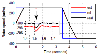
In fact, Angular speed is estimated from a sliding observer. Whereas, the measured stator voltage and currents are necessary for development the sensorless control algorithm. A reference speed of 300 rad / s was chosen for the simulation of the different operating regimes. In full operation, a load disturbance $\left(T_{L}=14 N . m\right)$ is applied in 1.5s and 2.5s.
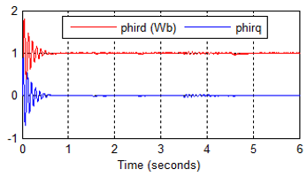
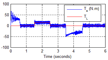
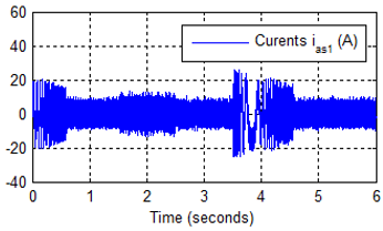
Then at t=3.5s an inversion of the rotational speed is made. Figure 4, 5 and 6, show the simulation results of the sliding observer for the sensorless vector control of DSIM.
Figure 4. Real and estimated speed
Figure 5. Rotor flux Flux in d-q axis
Figure 6. Electromagnetic torque
Figure 7. Currents in axis 1 $\left(i_{a s 1}\right)$
The results of the simulation show that the rotational speed can be estimated during the different operating regimes. The flux does not change in the presence of disturbances and perfectly follows the reference as well as for the speed. The observer used failed to obtain a low dynamic error and an almost zero static error.
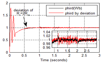
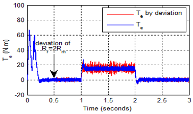
The sensitivity of the observer of the slip mode is tested against the parametric variations. Indeed, for the variation of rotor resistance was taken for a step of $+100 \% R_{r}$, from t=0.5s to 3s for a speed of 100 rad / s.
Figures 8, 9, 10 and 11 clearly show that the sliding mode speed observer is performing and its behavior is not affected.
Figure 8. Rotor speed
Figure 9. Rotor flux in -d- axis $\left(\Phi_{r d}\right)$
Finally, we can say that the carried sensorless can obtain high performances of robustness, stability and precision, in particular during the inversion of the speed and the variation of the parameters.
Figure 10. Electromagnetic torque
Figure 11. Estimation error $\left(\tilde{l}_{q s}\right)$
In this work, we have applied the Lyapunov stability method in the sensorless control of the DSIM by field oriented control (FOC) in sliding mode. Moreover, the estimation of the speed and flux is based on the "smooth" function which replaced the "sign" function, because the majority of researchers have observed that the "sign" function generates disturbances in torque and speed. The adopted control law has proven operating performance in terms of stability, robustness and rapidity of response.
Finally, the results encouraged us to estimate other parameters variations of the system like rotor resistance, the load torque..., and to more of noise sensitivity and complexity matrix error. We can also evaluate the performance of the two observers by series experimental in future work.
This work was supported by Electrical Engineering Laboratory (LGE) at the University of Mohamed Boudiaf- M’sila, (Algeria) and Signals & Systems Laboratory, Institute of Electrical and Electronic Engineering Boumerdes University, (Algeria). We like to thank Dr. Djalal Eddine Khodja and Dr. Salim Chakroune for their help in the preparation of this paper.
DSIM parameters
[1] Shoeb, H., Mohammad, A. (2016). Neural network observer design for sensorless control of induction motor drive. Science Direct, 49(1): 106-111. https://doi.org/10.1016/j.ifacol.2016.03.037
[2] Oscar, B. (2009). Sensorless vector control of induction motor drives based on artificial neural networks. Proceedings of the 7th IFAC Symposium on Fault Detection, Supervision and Safety of Technical Processes. Barcelona, Spain, 42(8): 185-190. https://doi.org/10.3182/20090630-4-ES-2003.00031
[3] Toufik, R., Chaouch, S., Saïd Naït-Saïd, M. (2016). Backstepping design for fault detection and FTC of an induction motor drives-based EVS. Journal for Control, Measurement, Electronics, Computing and Communications, 57(3): 736-748. https://doi.org/10.7305/automatika.2017.02.1733
[4] Yousfi, L., Lotfi, H., Abdelhani, B. (2017). Speed sensorless vector control of induction machine with Luenberger observer and Kalman filter. 4th International Conference on Control, Decision and Information Technologies (CoDIT). Barcelona, Spain, 0714-0720. https://doi.org/10.1109/CoDIT.2017.8102679
[5] Habibullah, M., Dah-Chuan, L. (2015). Speed-sensorless estimation for induction motors using extended Kalman filters. IEEE Transactions on Industrial Electronics, 62(3): 6765-6778. https://doi.org/10.3906/elk-1408-136
[6] Giorgio, B., Fridman, L., Usai, E. (2008). Modern sliding mode control theory. Springer Science & Business Media. ISBN 9783540790150.
[7] Li, J., Xu, L., Zhang, Z. (2005). An adaptive sliding-mode observer for induction motor sensorless speed control. IEEE Transactions on Industry Applications, 41(4): 1039-1046. https://doi.org/10.1109/TIA.2005.851585
[8] Montanari, M., Peresada, S., Tilli, A. (2006). A speed sensorless indirect field-oriented control for induction motors based on high gain speed estimation. Automatică, 42(10): 1637-1650. https://doi.org/10.1016/j.automatica.2006.05.021
[9] Chaaban, H., Djalaleddine, K., Salim, C. (2020). Sensorless backstepping control using an Luenberger observer for double star induction motor. Archives of Electrical Engineering, 69(1): 101-116. https://doi.org/10.24425/aee.2020.131761
[10] Wencen, J., Wang, Y. (2018). An adaptive Luenberger observer for speed-sensorless estimation of induction machines. Annual American Control Conference, Milwaukee, USA. https://doi.org/10.23919/ACC.2018.8431006
[11] Bennassar, A., Abbou, A., Akherraz, M., Barara, M. (2013). Sensorless Backstepping control using an adaptive Luenberger observer with three levels NPC inverter. International Journal of Electrical and Computer Engineering, 7(8): 1171-1177.
[12] Mouna, B., Lassaad, S. (2006). Speed sensorless indirect stator field oriented control of induction motor based on Luenberger observer. IEEE International Symposium on Industrial Electronics, Montreal, Quebec, Canada. https://doi.org/10.1109/ISIE.2006.295961
[13] Chaabane, H., Djalaleddine, K., Salim, C. (2019). Robust adaptive control of dual star asynchronous machine by reference model based on landau stability theorem. Advances in Modelling and Analysis C, 74(2): 56-62. https://doi.org/10.18280/ama_c.742-403
[14] Lazreg, M.H., Bentaallah, A. (2017). Speed sensorless vector control of double star induction machine using reduced order observer and MRAS estimator. The 5th International Conference on Electrical Engineering, Boumerdes, Algeria. https://doi.org/10.1109/ICEE-B.2017.8192150
[15] Tir, Z. (2017). Fuzzy logic field oriented control of double star induction motor drive. Electrical Engineering, 99(2): 495-503. https://doi.org/10.1007/s00202-016-0377-2
[16] Houari, K., Ahmed, B., Boubaker, B. (2018). Sliding-mode MRAS speed estimator for sensorless vector control of double stator induction motor. Majlesi Journal of Electrical Engineering, 12(3): 41-53.
[17] Hellali, L., Saad, B. (2018). Speed control of doubly star induction motor (DSIM) using direct field oriented control (DFOC) based on fuzzy logic controller (FLC). AMSE Journals, Advanced in Modelling and Analysis C, 73(4): 128-136. https://doi.org/10.18280/ama_c.730402
[18] Layadi, N., Zeghlache, S., Benslimane, T., Berrabah, F. (2017). Comparative analysis between the rotor flux oriented control and backstepping control of a double star induction machine (DSIM) under open-phase fault. AMSE Journals, Series Advances C, 72(4): 292-311. https://doi.org/10.18280/ama_c.720407
[19] Hellali, R., Zeghlache, S., Benalia, L., Layadi, N. (2018). Sliding mode control based on backstepping approach for a double star induction motor (DSIM). AMSE Journals, Advanced in Modelling and Analysis C, 73(4): 150-157. https://doi.org/10.18280/ama_c.730404
[20] Akkari, N., Chaghi, A., Abdessemed, R. (2014). Speed control of doubly star induction motor using direct torque DTC based to on model reference adaptive control (MRAC). International Journal of Hybrid Information Technologyy, 7(2): 19-28. http://dx.doi.org/10.14257/ijhit.2014.7.2.03